Abstract
Porous shallow-water equations (PSWE) are a mathematical model for urban flooding simulation that has gained popularity because of its modest computational burden. Under certain initial conditions, PSWE may admit multiple exact solutions. This implies that (i) a criterion is required to identify the unique physically relevant solution among the alternatives, and that (ii) the corresponding numerical models should incorporate this criterion. In the present paper, a procedure for the disambiguation of PSWE multiple exact solutions is proposed and a 1-d PSWE numerical scheme from the literature is modified to embed the disambiguation ability.
1. Introduction
Urban flood modeling is a challenging task because different spatial and time scales are involved in the hydrodynamic processes, due to the geometric complexity of the urban environment. Of course, a detailed solution of shallow-water equations (SWE) with the accurate modeling of all the buildings and obstacles may lead to excessively refined numerical grids, with an increase in the computational burden. Recently, porous shallow-water equations (PSWE) have been proposed to cope with this difficulty by treating the urban fabric as a porous medium where the obstacles are incorporated into the mathematical model itself.
From a mathematical point of view, PSWE are a system of non-strictly hyperbolic partial differential equations characterized by the presence of non-conservative products that model the interaction between fluid and obstacles. These non-conservative products are challenging because discontinuous solutions cannot be defined in the usual sense of distributions. In addition to this difficulty, it has been demonstrated that the PSWE Riemann problem is characterized by multiple exact solutions for certain classes of initial conditions. These alternative solutions are characterized by different flow depths and velocities, and they involve different energy-dissipation mechanisms [1], influencing the flood propagation celerity and the flood depth through the urban fabric [2]. This implies that a criterion must be introduced to select the unique, physically meaningful solution among the alternatives.
The finite volume numerical schemes available for the approximate solution of the PSWE model are usually based on the solution of a Riemann problem at cell interfaces [3,4,5,6,7,8]. Due to the existence of multiple mathematical solutions for the PSWE Riemann problem with certain initial conditions, a similar ambiguity is transferred to the PSWE numerical models based on the solution of a Riemann problem. This implies that different numerical models may converge to structurally different approximate solutions in the cases where multiple exact solutions are possible [9]. It is desirable that a numerical model for the approximate solution of the PSWE captures the unique physically meaningful solution among the alternatives.
Despite the results that are available in the literature, little importance has been attributed until now to modeling problems related to the existence of multiple solution in PSWE. In the present work, the physically meaningful solution of one-dimensional (1-d) PSWE for an example Riemann problem with multiple solutions is chosen after a comparison with the solution supplied by a 2-d SWE numerical model. Finally, this disambiguation rule is incorporated into an existing PSWE numerical scheme [3] and the corresponding numerical results are presented and discussed.
2. Mathematical Model
Under the assumption of horizontal bed and negligible friction, 1-d PSWE can be written as [2]:
In Equations (1) and (2), the meaning of the symbols is as follows: x and t are the longitudinal space coordinate and the time coordinate, respectively; is the porosity; is the vector of conserved variables, where is the flow depth; u is the longitudinal velocity; T is the matrix transpose symbol; and is a vector taking into account the forces exerted by the obstacles on the flow. In Equation (1), which is a vector equation that takes into account mass conservation and the second principle of Newton’s dynamics, the conserved variable vector u can be a discontinuous function. This allows modeling the discontinuities of the flow field (shocks) such as moving bores and standing hydraulic jumps. Of course, the geometry itself admits discontinuities, for example, through the boundaries between areas with different urban fabric densities. For this reason, the trivial Equation (2), stating that the porosity does not vary in time, has been added. The balance system of Equations (1) and (2) is not conservative, due to the presence of the non-conservative product . This means that the classic Rankine–Hugoniot Conditions, which define the moving shocks in conservative systems of hyperbolic equations, are meaningful for Equations (1) and (2) only if is continuous. In the case of discontinuous , flow discontinuities must be carefully defined case by case, using external physical knowledge [10].
The inspection of Equation (1) shows that 1-d PSWE formally coincide with 1-d SWE in a horizontal rectangular channel with variable width where the porosity is considered instead of the channel width. This mathematical identity is not fortuitous because the porosity of the PSWE model is a measure of the building density in urban areas. In particular, the reduction in porosity coincides with the increase in building density and then with the decrease in transverse space available for the flow passage.
2.1. Eigenstructure and Elementary Waves
For h > 0, the eigenvalues of the Jacobian associated with the system of Equations (1) and (2) are [3]
where is the Froude number. The corresponding eigenvectors, which are not written here for the sake of brevity, are reported in [3]. From Equation (3), it is evident that the PSWE are non-strictly hyperbolic on the hypersurfaces of the (h, u, φ) space. This introduces the possibility of multiple solutions for certain initial conditions.
We note that the PSWE 1- and 2-characteristic fields coincide with the corresponding characteristic fields of the ordinary 1-d SWE. This means that the elementary waves (shocks and rarefactions) associated with the 1- and 2-characteristic fields coincide with those of the 1-d SWE (see, for example, [11]). In particular, shock waves contained in the 1- or 2-characteristic fields are defined by means of the classic Rankine–Hugoniot Conditions.
2.2. Definition of Flow Discontinuities at Porosity Jumps
When the porosity is discontinuous, classic Rankine–Hugoniot Conditions cannot be used to define the corresponding flow discontinuities and a description of the discontinuity internal structure is needed [10]. In the present work, it will be assumed that geometric discontinuity consists of a region where the porosity varies monotonically. It is assumed that this region of rapid porosity variation is much shorter than the longitudinal scale of the urban flood propagation problem, ensuring that it can be safely modelled as a geometric discontinuity.
To complete the description of the discontinuity internal structure, it is assumed that, if u1 are u2 are the states immediately to the left and to the right of a porosity jump, respectively, and and are the corresponding porosities, the following is true [12]:
In Equation (4), ΔH is a loss of energy such that is always verified. From the physical point of view, Equation (4) expresses the fact that specific energy is invariant through the porosity jump, unless ΔH ≠ 0. When ΔH ≠ 0 is assumed, the corresponding dissipation physical mechanism needs to be specified. Finally, Equation (5) expresses the fact that discharge is invariant through the porosity discontinuity.
In the present paper, both of the two following alternatives are considered:
- (1)
- ΔH = 0; in this case, it is assumed that h and u vary smoothly through the discontinuity, keeping the flow character (subcritical or supercritical) unchanged; critical conditions may establish where porosity is minimum;
- (2)
- ΔH ≠ 0, and the hydraulic jump is chosen as a physical mechanism that is able to explain this energy loss; in this case, the supercritical flow entering the porosity discontinuity is reverted into a subcritical flow, and the flow is smooth through the porosity discontinuity with the exception of the hydraulic jump location; critical conditions may establish where porosity is minimum.
2.3. An Example of Multiple Solutions
This mathematical and physical analogy between the 1-d PSWE model and the 1-d SWE model in rectangular channels with variable width implies that the exact solutions found in [12] for the 1-d SWE model can be applied to the 1-d PSWE model as well. Consider the solution of the system of Equations (1) and (2) with the following discontinuous initial and geometric conditions (the Riemann problem):
In [12], it is demonstrated that this Riemann problem may admit (but not necessarily) a class of multiple solutions when and the flow from the right is supercritical with
The dimensionless numbers and are positive limit Froude numbers defined in [12] (not reported here for the sake of brevity). An additional class of multiple solutions is possible for and , but this possibility is neglected in the present work.
The following is considered the example where the states and the porosities in Equation (4) are , , , and . These initial conditions characterize a right supercritical flow that impacts on a porosity reduction and satisfies the condition of Equation (7). Supercritical flow conditions are also initially present to the left. The corresponding Riemann problem admits three different exact solutions (named S1, S2, and S3, respectively) that are plotted in Figure 1 (flow depth at time t = 5 s), where an arrow represents the flow direction through the porosity discontinuity.
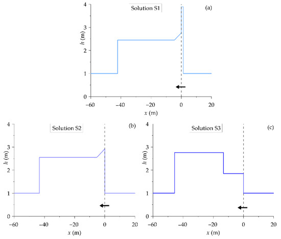
Figure 1.
Flow depth exact solution at time t = 5 s: (a) solution S1; (b) solution S2; and (c) solution S3.
The solution S1 (Figure 1a) is characterized by a right supercritical flow that enters a sudden porosity reduction in x = 0 and produces a reflected shock on the right, while the flow is partly transmitted on the left (left shock). A critical state is present immediately to the left of the porosity reduction, while the flow between the right shock and the porosity jump is subcritical. The energy is conserved through the porosity jump (ΔH = 0).
In solutions S2 (Figure 1b) and S3 (Figure 1c), there is no reflection of the supercritical flow from the right but only transmission. In solution S2 (Figure 1b), the incoming supercritical flow is reverted into subcritical by means of a hydraulic jump collocated inside the rapid porosity transition (ΔH ≠ 0), while critical conditions are found immediately to the left of the porosity discontinuity. In solution S3 (Figure 1c), the right flow remains supercritical through the porosity discontinuity (ΔH = 0), producing two advancing shocks on the left.
It is important to observe that solution multiplicity is not only caused by the use of two different flow discontinuity definitions (ΔH ≠ 0 or ΔH = 0). In fact, solutions S1 and S3 are both characterized by invariant energy (ΔH = 0) through the porosity discontinuity.
2.4. Rectangular Channel Analogy and Disambiguation of Multiple Solutions
Following the analogy between the 1-d PSWE model and the 1-d SWE model in rectangular channels with variable width, it is possible to reformulate the task of disambiguating the PSWE multiple solution as the task of disambiguating the multiple SWE solutions. Furthermore, we observe that the 1-d SWE model in horizontal rectangular channels with variable width is a simplification of the 2-d SWE model, where (i) a main flow direction is individuated, (ii) the flow velocity component transverse to the main flow direction is neglected, and (iii) the variations of flow depth and the parallel component of the flow velocity along the transverse direction are neglected. The loss of physical information due to the dimensional reduction of the 2-d SWE model initiates the emergence of multiple solutions in the 1-d SWE model, with the initial conditions specified in Equation (5). This suggests that, for a given problem, the comparison between the 2-d SWE solution and the 1-d SWE multiple solutions can be used to choose the unique physically relevant 1-d alternative.
The approximate solution of the example Riemann problem contained in Section 2.3 is tackled with the 2-d SWE numerical model described in [13] that considers a channel with length L = 200 m. The channel consists of a left reach, whose width is BL = 0.6 m, and a right reach, whose width is BR = 1 m (see Figure 2). A linear contraction, located at the center of the channel (where x = 0 m), connects the right reach to the left one by means of two straight walls that are inclined by 45° with respect to the street axis. The linear contraction, which is Lc = 0.20 m long, is sufficiently short with respect to the total length to be considered a true geometric discontinuity. A non-uniform unstructured triangular mesh is used, with an average size Δs = 0.50 m at the channel ends and Δs = 0.05 m in the vicinity of the contraction. All of the channel boundaries are free-slip walls, except for the left and right sides, which are open ends, and the initial conditions coincide with those of the 1-d model. The plane view of the flow depth around x = 0 is represented in Figure 2 at time t = 5 s.
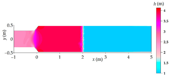
Figure 2.
Plan view of the water surface elevation with the reference 2-d SWE numerical model at t = 5 s around the channel contraction area. The flow is directed from right to left.
The inspection of Figure 2 shows that the supercritical flow from the right is only partially transmitted because a backward shock (the vertical line between the purple and cyan areas) moves towards the right. The flow, which is subcritical between the channel contraction and the moving right shock, accelerates through the contraction towards the critical state. From a comparison with Figure 1, it follows that the physically relevant 1-d solution of the example Riemann problem considered in Section 2.3 is S1.
3. Numerical Modeling
In this section, the original numerical model by [3] for 1-d PSWE and SWE with variable width is described, and it is shown how it can be modified to embed the solution disambiguation presented in Section 2.4.
3.1. 1-d Original Numerical Model
The 1-d physical domain of length L is subdivided in cells Ci (i = 1, 2,…, N) of length where the solution of the 1-d PSWE model of Equation (1) is approximated by the 1-d finite volume scheme
where
In Equations (8) and (9), the meaning of the symbols is as follows: is the time step; is the cell-averaged porosity in the cell Ci; is the cell-averaged vector u in the cell Ci; is the numerical flux corresponding to the exact or approximate solution of the 1-d SWE problem for the initial left and right states v and w; is an approximation of the porosity at the interface between the cells Ci and Ci+1; and are appropriate approximations of the conserved variables immediately to the left and to the right of the interface between cells Ci and Ci+1; and are the contributions to the cell Ci exerted by the porosity discontinuities at the interfaces i-1/2 and i+1/2, respectively. In the original numerical model by [3], the variables and are reconstructed at each time step from the variables and , respectively, using the assumption of invariant energy and discharge and maintaining the character of the flow (subcritical or supercritical), as follows:
More details about the treatment of variable reconstruction at interfaces when the energy available is not sufficient are reported in [3]. The solution of Equation (1) with the initial conditions described in Section 2.3 is approximated with the scheme by [3] using Δx = 0.20 m and Δt = 0.005 s. The corresponding numerical results (flow depth h) at time t = 5 s are plotted in Figure 3 with a dashed line.
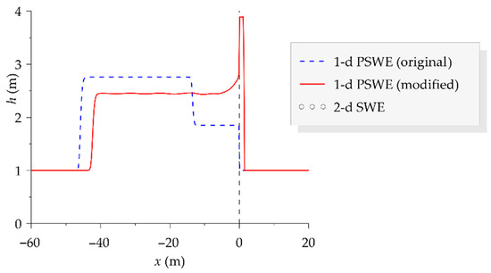
Figure 3.
Profile view of the water surface elevation at t = 5 s: 1-d PSWE numerical model by [3] (dashed blue line); modified 1-d PSWE model (continuous red line); and reference 2-d SWE numerical model (circles). The flow is directed from right to left.
The comparison between Figure 1 and Figure 3 shows that that the numerical model by [3] (dashed blue line) captures solution S3 (Figure 1c), which is characterized by supercritical flow through the porosity reduction. In hindsight, this is easily understood since the variable reconstruction described by [3] preserves the supercritical character of the flow coming from the right. In Figure 3, a profile view of the flow depth supplied by the 2-d SWE model (circles) is also represented. The inspection of the figure makes the shape of the S1 solution evident, with a backward shock to the right of the contraction and a critical state immediately to the left of the geometric discontinuity.
3.2. 1-d Modified Numerical Model
The original model by [3] is modified to embed the disambiguation mechanism suggested by the 2-d SWE model. In case Equation (7) is satisfied, an additional variable reconstructed at the interface i+1/2 is introduced. The reconstructed variables , and are calculated with an iterative process by imposing the following conditions:
- the discharge and the energy corresponding to coincides with those corresponding to , as already made in Equation (10);
- is critical;
- is connected to by a shock contained into the second characteristic field;
- and are connected by the condition of discharge and energy invariance, like in Equation (11);
- The contribution is calculated as:
The results of the modified 1-d PSWE numerical model are represented in Figure 3 with a continuous red line. The inspection of the Figure shows that the shape of the S1 solution is nicely captured. In particular, the strength and position of the moving waves (rarefactions and shocks) compare well with those supplied by the 2-d SWE numerical model, while the maximum flow depth, immediately to the right of the geometric discontinuity, is satisfactorily predicted.
4. Conclusions
Porous shallow-water equations are a non-conservative system of hyperbolic equations that has recently gained popularity for flooding simulation in urban areas. Finite-volume models for the approximate solution of the porous shallow-water equations are mainly based on the approximate solution of a local Riemann problem. Under certain initial conditions, this Riemann problem may admit multiple exact solutions. Of course, it is desirable that only the physically meaningful Riemann solution, among the alternatives, is used for flooding computations. In the present paper, it has been shown that a physical analogy can be established between 1-d porous shallow-water equations and 1-d shallow-water equations in rectangular channels with variable width. Recalling that the 1-d shallow-water equations model is nothing but a simplification of the 2-d shallow-water equations model, the 2-d model has been used here to disambiguate multiple 1-d solutions by reintroducing the missing physical information. Of course, 1-d porous shallow-water equations numerical models should be able to capture the physically relevant numerical solution. For this reason, a reference numerical model from the literature [3] has been studied, showing why it does not supply the physically meaningful solution and how a modification can be introduced to correct this behavior. The solution disambiguation process and the corresponding numerical implementation outlined here have never been applied before in the field of flood modeling, but the preliminary results seem encouraging. In the present paper, only one example Riemann problem has been considered, but the general task of disambiguating the multiple Riemann solution to porous shallow-water equations will be considered in the future.
Author Contributions
Conceptualization, L.C. and G.V.; methodology, L.C. and G.V.; software, G.V.; validation, G.V.; formal analysis, L.C. and G.V.; investigation, G.V.; resources, R.D.M.; data curation, G.V.; writing—original draft preparation, L.C., G.V., and R.D.M.; supervision, R.G. and R.D.M.; project administration, L.C.; and funding acquisition, L.C. All authors have read and agreed to the published version of the manuscript.
Funding
The research project “Sistema di supporto decisionale per il progetto di casse di espansione in linea in piccoli bacini costieri” was funded by the Italian Ministry for Environment, Land, and Sea Protection through the funding program “Metodologie per la valutazione dell’efficacia sulla laminazione delle piene in piccoli bacini costieri di sistemi di casse d’espansione in linea realizzate con briglie con bocca tarata”.
Conflicts of Interest
The authors declare no conflict of interest.
References
- Cozzolino, L.; Castaldo, R.; Cimorelli, L.; Della Morte, R.; Pepe, V.; Varra, G.; Covelli, C.; Pianese, D. Multiple solutions for the Riemann problem in the Porous Shallow water Equations. In Proceedings of the HIC 2018 13th International Conference on Hydroinformatics, Palermo, Italy, 1–7 July 2018; pp. 476–484. [Google Scholar] [CrossRef]
- Varra, G.; Pepe, V.; Cimorelli, L.; Della Morte, R.; Cozzolino, L. On integral and differential porosity models for urban flooding simulation. Adv. Water Resour. 2020, 136, 103455. [Google Scholar] [CrossRef]
- Castro, M.J.; Pardo Milanés, A.; Parés, C. Well-balanced numerical schemes based on a generalized hydrostatic reconstruction technique. Math. Model. Methods Appl. Sci. 2007, 17, 2055–2113. [Google Scholar] [CrossRef]
- Guinot, V.; Soares-Frazão, S. Flux and source term discretization in 2-d shallow water models with porosity on unstructured grids. Int. J. Numer. Methods Fluids 2006, 50, 309–345. [Google Scholar] [CrossRef]
- Sanders, B.F.; Schubert, J.E.; Gallegos, H.A. Integral formulation of shallow-water equations with anisotropic porosity for urban flood modelling. J. Hydrol. 2008, 362, 19–38. [Google Scholar] [CrossRef]
- Ferrari, A.; Vacondio, R.; Dazzi, S.; Mignosa, P. A 1D-2D shallow water equations solver for discontinuous porosity field based on a generalized Riemann problem. Adv. Water Resour. 2017, 107, 233–249. [Google Scholar] [CrossRef]
- Guinot, V.; Sanders, B.F.; Schubert, J.E. Dual integral porosity shallow water model for urban flood modelling. Adv. Water Resour. 2017, 103, 16–31. [Google Scholar] [CrossRef]
- Cozzolino, L.; Pepe, V.; Cimorelli, L.; D’Aniello, A.; Della Morte, R.; Pianese, D. The solution of the dam-break problem in the Porous Shallow water Equations. Adv. Water Resour. 2018, 114, 83–101. [Google Scholar] [CrossRef]
- Andrianov, N. Performance of numerical methods on the non-unique solution to the Riemann problem for the shallow water equations. Int. J. Numer. Methods Fluids 2005, 47, 825–831. [Google Scholar] [CrossRef]
- LeFloch, P.G. Shock Waves for Nonlinear Hyperbolic Systems in Nonconservative Form, Preprint 593; Institute for Mathematics and Its Applications: Minneapolis, MN, USA, 1989. [Google Scholar]
- Toro, E.F. Shock-Capturing Methods for Free-Surface Shallow Flows; Wiley: Chichester, UK, 2001. [Google Scholar]
- Varra, G.; Pepe, V.; Cimorelli, L.; Della Morte, R.; Cozzolino, L. The exact solution to the Shallow water Equations Riemann problem at width jumps in rectangular channels. Adv. Water Resour. 2021, 155, 103993. [Google Scholar] [CrossRef]
- Pepe, V.; Cimorelli, L.; Pugliano, G.; Della Morte, R.; Pianese, D.; Cozzolino, L. The solution of the Riemann problem in rectangular channels with constrictions and obstructions. Adv. Water Resour. 2019, 129, 146–164. [Google Scholar] [CrossRef]


Publisher’s Note: MDPI stays neutral with regard to jurisdictional claims in published maps and institutional affiliations. |
© 2022 by the authors. Licensee MDPI, Basel, Switzerland. This article is an open access article distributed under the terms and conditions of the Creative Commons Attribution (CC BY) license (https://creativecommons.org/licenses/by/4.0/).