
Return Periods in Assessing Climate Change Risks: Uses and Misuses †


1
Department of Tourism Management, School of Administrative, Economic and Social Sciences, University of West Attica, 12243 Egaleo, Greece
2
Department of Trade, Shipping and Transport, School of Management Science, University of the Aegean, 82132 Chios, Greece
†
Presented at the 16th International Conference on Meteorology, Climatology and Atmospheric Physics—COMECAP 2023, Athens, Greece, 25–29 September 2023.
Environ. Sci. Proc. 2023, 26(1), 75; https://doi.org/10.3390/environsciproc2023026075
Published: 25 August 2023
(This article belongs to the Proceedings of 16th International Conference on Meteorology, Climatology and Atmospheric Physics—COMECAP 2023)
Abstract
:Return periods (Ts) are used to estimate the interval of time between natural hazard occurrences of a certain size and assess the risks associated with hydrological occurrences, climate extremes, structural failures and seismicity. Despite Ts being widely used, they are characterized by strong misconceptions and ambiguities. Moreover, although they have been successfully used when discussing storm surges, high tides and extreme precipitation, concerns arise from their use in assessing probabilities of future global mean sea level rise (SLR). Most papers discuss SLR return periods considering storm surges or high tides and not SLR itself, as a separate and unique hazard. Sea level rise due to storm surges or tides is regional and temporary and differs from the global SLR, which is a long lasting and slow phenomenon. This paper discusses these misconceptions and misuses of return periods in assessing flood risk and the probability of sea level rise at the global level and suggests a method for assessing likelihoods of climate change risks that can be widely accepted and commonly used by all stakeholders and decision makers for all types of climate hazards.
1. Introduction
The return period (or recurrence interval) (T) is the “average time until the next occurrence of a defined event” [1] or “an estimate of the interval of time between events of a certain intensity or size” [2], and is expressed by the following formula:
where P(X ≥ x), is the probability of occurrence of a hydrological variable X of an equal or greater magnitude x in a given time interval [3].
T = 1/P(X ≥ x)
Return periods have been widely used to assess the probability of occurrence of most natural hazards, such as earthquakes [4], tsunamis [5], extreme heat/cold weather occurrences [6,7,8], extreme precipitation [9,10], storm surges [11], tropical/extratropical cyclones [12], landslides [13].
Return periods are also used to assess (i) failures of hydrological safety systems due to extreme hydrological occurrences [14], (ii) failures of buildings [15] and critical infrastructure such as bridges [16] and highways [17] due to climate extremes, (iii) seismic resistance construction decisions [18], etc.
Despite the concept of return period being widely used in assessing the risks of hydrological and geophysical hazards, there are still strong misconceptions that could lead to wrong estimations [19]. Phrases such as “The 50-year return period flood peak of 100 m3s−1 occurs once every 50 years’’ or ‘‘A flood peak of 100 m3s−1” means that the value of 100 m3s−1 has 50-year return period” are very common, but completely wrong [19]. The return period does not mean that an event of a given size and magnitude will occur at intervals of T years on a regular basis, or that an event that has already occurred will not occur again in the next T years [3].
Return period estimation is based on the study of historical data of a specific event. An example of an extreme event is discussed below, so as to make clear what a return period is and what the probability of occurrence is for this specific event of this magnitude.
Let us assume a climate extreme X that exceeded magnitude x eight times during the period 1975–2018 (Table 1). According to Table 1, recurrence intervals range from 1 year to 16 years [20].
By applying the average return period of X that exceeds x, which is equal to 5.1 years, to the return period formula, the probability of climate hazard X to exceed x is approximately 20%. This means that a 5.1-year event has approximately a 20% probability in any year and it is possible to have more than one such event within a year or even months [2]. The relation between the probability of occurrence of a value of a variable X equal to or greater than x in any year and the return period is given in Table 2 [1]:
Based on the above, the return period is in fact nonsense when it is used to assess the probability of occurrence of an event that has large recurrence intervals, e.g., T > 10,000, as probabilities are eventually zero. As a result, the return period is not the appropriate tool for assessing risks of all climate hazards, as probability assessment is vital for accurate risk assessments and effective decision making. This paper aims to identify the ambiguities deriving from the use of return periods in the assessment of flood risks, driven from sea level rise (SLR), storm surges, high tides, tropical cyclones and extreme precipitation.
2. Materials and Methods
This paper concerns a review of 127 peer review papers from the Scopus database which use return periods as a tool for studying sea level rise impacts, coastal vulnerabilities, extreme precipitation impact, storm surges, high tides and flood risk.
The analysis of the research papers using return periods (both bivariate and univariate) in the study of flood related vulnerabilities, impacts and risk, generates a series of inconsistencies and ambiguities that are further discussed below. The return period’s misuse in scientific research highlights the need for a widely accepted method that could be easily comprehended and used by all risk managers, stakeholders and decision makers when assessing climate change risks.
3. Results
The majority of the papers (57%) concern SLR and extreme precipitation (40%). The largest portion of the papers (86%) concerning SLR return periods (TSLR) mainly discuss return periods of storm surges (Tstorm surge) and high tides (Thigh tide) (Figure 1). Storm surges alone, separate from SLR hazards, are studied in 31% of the research papers, while flood return period studies cover 28% of the total studies. The return periods of combined SLR and extreme precipitation risk was studied by 18% of the papers, but SLR is also discussed mainly from storm surges perspective. River water rise due to extreme precipitation is very rarely discussed, despite the fact that riverine flooding is widely discussed (Figure 1).
According to the literature findings, although extreme precipitation is one of the basic factors of inundation, the return periods of precipitation and flooding occurrences are not equivalent [21]. For reasons that have not yet been well comprehended or scientifically proved, the return period of inundation is always greater than the return period of precipitation [22]. In order to display similar return periods, they have to occur only under very low probabilities and under exactly the same conditions [21]. Among others, regional climatological features, soil moisture characteristics before the rainfall and soil evaporation, soil water storage capacity, precipitation spatial distribution, precipitation intensity and duration are factors that effect the relationship between precipitation and flood return periods [21,23].
Moreover, in most cases, when discussing SLR return period, authors refer to storm surges, high tides or waves and not the sea level rise itself [24,25]. Indeed, storm surges, high tides and wind waves contribute significantly to the level of the sea [26], but they do not define the global mean sea level, as they display high variability from place to place and follow the specific climatic features of each region and specific duration, intensity and frequency [27,28]. Ice and glaciers thawing are the primary contributors to global SLR acceleration [29], which will cause the most significant impact on future coastal populations, systems and infrastructure [30], and not storm surges or high waves, which are regional and temporary climate extremes.
Sea levels have changed dramatically through five glacial cycles [31] (Figure 2), ranging from approximately −120 to approximately 10 m, with zero sea level to represent the present years (Figure 2a). Based on the sea level cycles of the previous 500,000 years (Figure 2a), sea level takes several thousand years to reach present sea levels, and SLR remains a phenomenon that has been progressing slowly over the years [32]. More precisely, existing (present) sea levels were exceeded sometime during the last 1000–3000 years, and once again approximately 120,000 years ago. There are no data for the years before the last 500,000 years, which means that it may have occurred even millions of years earlier. Thus, sea level rise itself (not storm surges or high waves) displays very large return periods, and the probability of occurrence is close to zero. More precisely, P(SLR ≥ SLRpresent) ≈ 0, for any T > 1000 years
Even if it is considered that sea level has exceeded present levels during the last 2000–5000 years, approximately (Figure 2b), the fact that the previous interval occurrence lasted more than 120,000 years means that the average return period will be very high and the probability of occurrence will remain close to zero. On the contrary, storm surges perform higher frequencies and smaller return periods. For instance, in Northeastern USA, for a return period of 10 years, storm surge return levels could range from 0.9 to 1.5 m, while for a 50-year return period, the storm surge return level could range from 1.1 to 2.1 m [11].
Most hydrological series cover a period of about 30–50 years [35], while the same period does not provide the same important information about global SLR with respect to return periods. As illustrated by Figure 2b, there is no interval occurrence that can be assessed during the period of 50 years, 100, 200, or even 1000 years, as sea levels have never exceeded the present sea level over these periods. The SLR trend is increasing and is expected to increase more in the future due to global heating.
4. Discussion and Conclusions
According to the above, although return periods are a widely accepted tool for assessing flood-related risks, they cannot be used to define the probability of global mean sea level rise (MSLR). Giving a probability of MSLR occurrence close to zero means that SLR risk is negligible, which is an absurd and invalid concept. As the literature is mainly built upon the consideration that SRL, storm surges and high waves contribute similarly to SLR risk and coastal flooding, the above observation makes it necessary for researchers to re-define the use of return periods when assessing SLR risk.
In order to overcome the inconsistencies from the use of return periods in assessing flood risks, this research recommends that probabilities should follow the qualitative approach adopted by IPCC reports, ranging from “Exceptionally Unlikely” to “Virtual certain” [36,37,38], combined with the level of confidence [39], and which describes the validity of the related findings. A level of confidence that ranges from“ Very high confidence” to “Very low confidence” can affect the meaning of the probability [40]. According to them, when an event is given a high or virtually certain likelihood, it must have a high confidence and never low confidence, or else it is not possible to be interpreted in a meaningful way. By assigning metrics on a scale [1,10] (Table 3), probabilities absorb degrees of confidence, increasing their accuracy.
So, when IPCC reports say that SLR in Japan is “likely” to occur with “medium confidence”, the proposed probability scale level is assigned as “7”, while, in the case of extreme precipitation that is “extremely likely” to occur with “very high confidence”, the probability scale is equal to “10”.
To summarize, instead of using return periods to assess flood risk, probability scales would result in more accurate risk assessment, as they are easy to comprehend and can be widely used by all stakeholders and decision makers. Return periods can be used to assess risk to extreme precipitation, storm surges and high tides but not future sea level rise at a global level. The use of probability scales could lead to more realistic results which are essential for coastal adaptation and resilience, by eliminating errors in calculation related to the more complex and ambiguous probabilistic approach of return periods.
Funding
This research received no external funding.
Institutional Review Board Statement
Not applicable.
Informed Consent Statement
Not applicable.
Data Availability Statement
Data sharing not applicable. No new data were created or analyzed in this study. Data sharing is not applicable to this article.
Conflicts of Interest
The author declares no conflict of interest.
References
- American Meteorology Society Glossary. Available online: https://glossary.ametsoc.org/wiki/Return_period (accessed on 5 December 2022).
- Deraman, W.H.A.W.; Mutalib, N.J.A.; Mukhtar, N.Z. Determination of return period for flood frequency analysis using normal and related distributions. J. Phys. Conf. Ser. 2017, 890, 012162. [Google Scholar] [CrossRef]
- Rakhecha, P.R.; Singh, V.P. Applied Hydrometeorology; Springer: Heidelberg, Germany, 2009. [Google Scholar]
- Baaqeel, A.; Quliti, S.; Daghreri, Y.; Hajlaa, S.; Yami, H. Estimating the Frequency, Magnitude and Recurrence of Extreme Earthquakes in Gulf of Aqaba, Northern Red Sea. Open J. Earthq. Res. 2016, 5, 135–152. [Google Scholar] [CrossRef]
- Kulikov, E.; Rabinovich, A.; Thomson, R. Estimation of Tsunami Risk for the Coasts of Peru and Northern Chile. Nat. Hazards 2005, 35, 185–209. [Google Scholar] [CrossRef]
- Dosio, A.; Mentaschi, L.; Fischer, E.; Wyser, K. Extreme heat waves under 1.5 °C and 2 °C global warming. Environ. Res. Lett. 2018, 13, 054006. [Google Scholar] [CrossRef]
- Wehner, M.F. Characterization of long period return values of extreme daily temperature and precipitation in the CMIP6 models: Part 2, projections of future change. Weather. Clim. Extrem. 2020, 30, 100284. [Google Scholar] [CrossRef]
- Otto, F.E.L.; Philip, S.; Kew, S.; Li, S.; King, A.; Cullen, H. Attributing high-impact extreme events across timescales—A case study of four different types of events. Clim. Change 2018, 149, 399–412. [Google Scholar] [CrossRef]
- Kumari, S.; Haustein, K.; Javid, H.; Burton, C.; Allen, M.R.; PAltan, H.; Dadson, S.; Otto, F.E.L. Return period of extreme rainfall substantially decreases under 1.5 °C and 2.0 °C warming: A case study for Uttarakhand, India Environ. Res. Lett. 2019, 14, 044033. [Google Scholar] [CrossRef]
- Pandey, S.; Mishra, B.K. Spatial and Temporal Analysis of Extreme Precipitation under Climate Change over Gandaki Province, Nepal. Architecture 2022, 2, 724–759. [Google Scholar] [CrossRef]
- Lin, N.; Marsooli, R.; Colle, B.A. Storm surge return levels induced by mid-to-late-twenty-first-century extratropical cyclones in the Northeastern United States. Clim. Change 2019, 154, 143–158. [Google Scholar] [CrossRef]
- Dullaart, J.C.M.; Muis, S.; Bloemendaal, N.; Chertova, M.V.; Couasnon, A.; Aerts, J.C.J.H. Accounting for tropical cyclones more than doubles the global population exposed to low-probability coastal flooding. Commun. Earth Environ. 2021, 2, 135. [Google Scholar] [CrossRef]
- Tsunetaka, H. Comparison of the return period for landslide-triggering rainfall events in Japan based on standardization of the rainfall period. Earth Surf. Process. Landf. 2021, 46, 2984–2998. [Google Scholar] [CrossRef]
- Volpi, E.; Fiori, A.; Grimaldi, S.; Lombardo, F.; Koutsoyiannis, D. Save hydrological observations! Return period estimation without data decimation. J. Hydrol. 2019, 571, 782–792. [Google Scholar] [CrossRef]
- Li, S.H. Design Wind Speed for Buildings and Facilities With Non-Standard Design Life in Canadian Wind Climates. Front. Built Environ. 2022, 8, 829533. [Google Scholar] [CrossRef]
- Pizarro, A.; Manfreda, S.; Tubaldi, E. The Science behind Scour at Bridge Foundations: A Review. Water 2020, 12, 374. [Google Scholar] [CrossRef]
- Meyer, M.; Flood, M.; Keller, J.; Lennon, J.; McVoy, G.; Dorney, C.; Leonard, K.; Hyman, R.; Smith, J. The Transportation Research Board (TRB) National Cooperative Highway Research Program (NCHRP) Report 750: Strategic Issues Facing Transportation, Volume 2: Climate Change, Extreme Weather Events, and the Highway System: Practitioner’s Guide and Research Report; National Academy of Sciences: Washington, DC, USA, 2014. [Google Scholar]
- Tsompanakis, Y. Earthquake Return Period and Its Incorporation into Seismic Actions. In Encyclopedia of Earthquake Engineering; Beer, M., Kougioumtzoglou, I.A., Patelli, E., Au, S.K., Eds.; Springer: Berlin/Heidelberg, Germany, 2015. [Google Scholar] [CrossRef]
- Serinaldi, F. Dismissing return periods! Stoch. Environ. Res. Risk Assess. 2014, 29, 1179–1189. [Google Scholar] [CrossRef]
- Van Westen, C.J.; Jetten, V.; Alkema, D.; Brussel, M. Development of the Caribbean Handbook on Disaster Risk Information Management. 2014. Available online: https://www.cdema.org/virtuallibrary/index.php/charim-hbook/methodology/2-analysing-hazards/2-3-rainfall-analysis (accessed on 1 December 2020). [CrossRef]
- Vangelis, H.; Zotou, I.; Kourtis, I.M.; Bellos, V.; Tsihrintzis, V.A. Relationship of Rainfall and Flood Return Periods through Hydrologic and Hydraulic Modeling. Water 2022, 14, 3618. [Google Scholar]
- Viglione, A.; Blöschl, G. On the role of storm duration in the mapping of rainfall to flood return periods. Hydrol. Earth Syst. Sci. 2009, 13, 205–216. [Google Scholar] [CrossRef]
- Osei, M.A.; Amekudzi, L.K.; Omari-Sasu, A.Y.; Yamba, E.I.; Quansah, E.; Aryee, J.N.A.; Preko, K. Estimation of the return periods of maxima rainfall and floods at the Pra River Catchment, Ghana, West Africa using the Gumbel extreme value theory. Heliyon 2021, 7, e06980. [Google Scholar] [CrossRef]
- Paulik, R.; Stephens, S.; Wild, A.; Wadhwa, S.; Bell, R.G. Cumulative building exposure to extreme sea level flooding in coastal urban areas. Int. J. Disaster Risk Reduct. 2021, 66, 102612. [Google Scholar] [CrossRef]
- Kirezci, E.; Young, I.R.; Ranasinghe, R.; Muis, S.; Nicholls, R.J.; Lincke, D.; Hinkel, J. Projections of global-scale extreme sea levels and resulting episodic coastal flooding over the 21st Century. Sci. Rep. 2020, 10, 11629. [Google Scholar] [CrossRef]
- Marcos, M.; Rohmer, J.; Vousdoukas, M.I.; Mentaschi, L.; Le Cozannet, G.; Amores, A. Increased extreme coastal water levels due to the combined action of storm surges and wind waves. Geophys. Res. Lett. 2019, 46, 4356–4364. [Google Scholar] [CrossRef]
- Ezer, T. Sea level acceleration and variability in the Chesapeake Bay: Past trends, future projections, and spatial variations within the Bay. Ocean. Dyn. 2023, 73, 23–34. [Google Scholar] [CrossRef]
- Petroliagkis, T.I. Estimations of statistical dependence as joint return period modulator of compound events–Part 1: Storm surge and wave height. Nat. Hazards Earth Syst. Sci. 2018, 18, 1937–1955. [Google Scholar] [CrossRef]
- van der Linden, E.C.; Le Bars, D.; Lambert, E.; Drijfhout, S. Antarctic contribution to future sea level from ice shelf basal melt as constrained by ice discharge observations. Cryosphere 2023, 17, 79–103. [Google Scholar] [CrossRef]
- Cazenave, A.; Palanisamy, H.; Ablain, M. Contemporary sea level changes from satellite altimetry: What have we learned? What are the new challenges? Adv. Space Res. 2018, 62, 1639–1653. [Google Scholar]
- Grant, K.; Rohling, E.; Ramsey, C.; Cheng, H.; Edwards, R.L.; Florindo, F.; Heslop, D.; Marra, F.; Roberts, A.P.; Tamisiea, M.E.; et al. Sea-level variability over five glacial cycles. Nat. Commun. 2014, 5, 5076. [Google Scholar] [CrossRef]
- Taherkhani, M.; Vitousek, S.; Barnard, P.L.; Frazer, N.; Anderson, T.R.; Fletcher, C.H. Sea-level rise exponentially increases coastal flood frequency. Sci. Rep. 2020, 10, 6466. [Google Scholar] [CrossRef]
- Available online: https://www.climate.gov/news-features/understanding-climate/climate-change-global-sea-level (accessed on 2 February 2023).
- Donoghue, J.F. Sea level history of the northern Gulf of Mexico coast and sea level rise scenarios for the near future. Clim. Change 2011, 107, 17–33. [Google Scholar] [CrossRef]
- Van Campenhout, J.; Houbrechts, G.; Peeters, A.; Petit, F. Return Period of Characteristic Discharges from the Comparison between Partial Duration and Annual Series, Application to the Walloon Rivers (Belgium). Water 2020, 12, 792. [Google Scholar] [CrossRef]
- Handmer, J.; Honda, Y.; Kundzewicz, Z.W.; Arnell, N.; Benito, G.; Hatfield, J.; Mohamed, I.F.; Peduzzi, P.; Wu, S.; Sherstyukov, B.; et al. Changes in impacts of climate extremes: Human systems and ecosystems. In Managing the Risks of Extreme Events and Disasters to Advance Climate Change Adaptation; Field, C.B., Barros, V., Stocker, T.F., Qin, D., Dokken, D.J., Ebi, K.L., Mastrandrea, M.D., Mach, K.J., Plattner, G.-K., et al., Eds.; A Special Report of Working Groups I and II of the Intergovernmental Panel on Climate Change (IPCC); Cambridge University Press: Cambridge, UK; New York, NY, USA, 2012; pp. 231–290. [Google Scholar]
- Jevrejeva, S.; Frederikse, T.; Kopp, R.E.; Le Cozannet, G.; Jackson, L.P.; van de Wal, R.S.W. Probabilistic Sea Level Projections at the Coast by 2100. Surv. Geophys. 2019, 40, 1673–1696. [Google Scholar] [CrossRef]
- IPCC. Intergovernmental Panel for Climate Change (IPCC), 2014: Climate Change 2014: Synthesis Report. Contribution of Working Groups I, II and III to the Fifth Assessment Report of the Intergovernmental Panel on Climate Change; Core Writing Team, Pachauri, R.K., Meyer, L.A., Eds.; IPCC: Geneva, Switzerland, 2014; 151p. [Google Scholar]
- Mastrandrea, M.D.; Field, C.B.; Stocker, T.F.; Edenhofer, O.; Ebi, K.L.; Frame, D.J.; Held, H.; Kriegler, E.; Mach, K.J.; Matschoss, P.R.; et al. Guidance Note for Lead Authors of the IPCC Fifth Assessment Report on Consistent Treatment of Uncertainties. In Proceedings of the IPCC Cross-Working Group Meeting on Consistent Treatment of Uncertainties, Jasper Ridge, CA, USA, 6–7 July 2010. [Google Scholar]
- Kandlikar, M.; Risbey, J.; Dessai, S. Representing and communicating deep uncertainty in climate-change assessments. Comptes Rendus Geosci. 2005, 337, 443–455. [Google Scholar] [CrossRef]
Figure 1.
Peer-reviewed papers concerning the return period of flood-related hazards. (a). Papers distribution by climate hazard; (b) Papers studying combined hazards.
Figure 1.
Peer-reviewed papers concerning the return period of flood-related hazards. (a). Papers distribution by climate hazard; (b) Papers studying combined hazards.
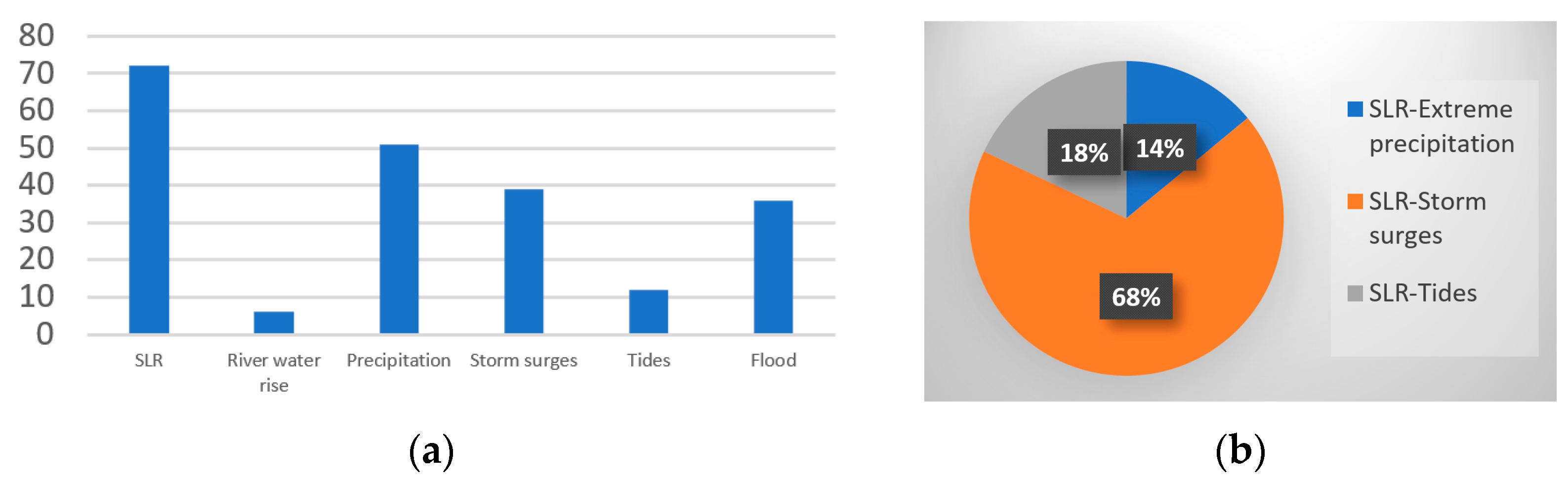
Figure 2.
Sea level cycles [33,34]. (a). Sea level cycles during the past 500,000 years [33], (b). Global Sea Level Trend for the period 1980–present [34].


Table 1.
Return period assessment.
| Years When the Magnitude of Climate Hazard X Exceeded Level x, during 1975–2018 | 1980 | 1981 | 1982 | 1998 | 2001 | 2007 | 2012 | 2017 | Average |
|---|---|---|---|---|---|---|---|---|---|
| Return Period (T) | 4 years (1966–1970) | 1 year (1970–1971) | 1 year (1971–1972) | 16 years (1973–1988) | 3 years (1989–1991) | 6 years (1991–1997) | 5 years (1997–2002) | 5 years (2002–2007) | 5.1 years |
Table 2.
Return period and probability relation.
| Return Period (T) | |||||||||||||
|---|---|---|---|---|---|---|---|---|---|---|---|---|---|
| 10,000 | 2000 | 1000 | 200 | 100 | 50 | 20 | 10 | 5 | 3 | 2 | 1.5 | 1 | |
| Probability (%) | 0.01 | 0.05 | 0.1 | 0.5 | 1 | 2 | 5 | 10 | 20 | 33 | 50 | 66 | 100 |
Table 3.
Numerical scale for Probability of Occurrence.
| Qualitative Assessment of Likelihood | Associated Likelihood | Degree of Confidence | Probability Scale |
|---|---|---|---|
| Virtually certain/ Extremely likely | >99%/>95% | High confidence | 10 |
| Very likely | >90% | High confidence | 9 |
| Likely | >66% | High confidence/Medium confidence | 8/7 |
| About as likely as not | 33–66% | High confidence/Medium confidence | 6/5 |
| Unlikely | <33% | Medium Confidence/High confidence | 4/3 |
| Very unlikely | <10% | High Confidence | 2 |
| Extremely unlikely/Exceptionally Unlikelly | <5%/<1% | High Confidence | 1 |
Disclaimer/Publisher’s Note: The statements, opinions and data contained in all publications are solely those of the individual author(s) and contributor(s) and not of MDPI and/or the editor(s). MDPI and/or the editor(s) disclaim responsibility for any injury to people or property resulting from any ideas, methods, instructions or products referred to in the content. |
© 2023 by the author. Licensee MDPI, Basel, Switzerland. This article is an open access article distributed under the terms and conditions of the Creative Commons Attribution (CC BY) license (https://creativecommons.org/licenses/by/4.0/).
Share and Cite
MDPI and ACS Style
Koliokosta, E. Return Periods in Assessing Climate Change Risks: Uses and Misuses. Environ. Sci. Proc. 2023, 26, 75. https://doi.org/10.3390/environsciproc2023026075
AMA Style
Koliokosta E. Return Periods in Assessing Climate Change Risks: Uses and Misuses. Environmental Sciences Proceedings. 2023; 26(1):75. https://doi.org/10.3390/environsciproc2023026075
Chicago/Turabian StyleKoliokosta, Efthymia. 2023. "Return Periods in Assessing Climate Change Risks: Uses and Misuses" Environmental Sciences Proceedings 26, no. 1: 75. https://doi.org/10.3390/environsciproc2023026075