Real Driving Emissions—Event Detection for Efficient Emission Calibration

Abstract

The systematic analysis of measurement data allows a large amount of information to be obtained from existing measurements in a short period of time. Especially in vehicle development, many measurements are performed, and large amounts of data are collected in the process of emission calibration. With the introduction of Real Driving Emissions Tests, the need for targeted analysis for efficient and robust calibration of a vehicle has further increased. With countless possible test scenarios, test-by-test analysis is no longer possible with the current state-of-the-art in calibration, as it takes too much time and can disregard relevant data when analyzed manually. In this article, therefore, a methodology is presented that automatically analyzes exhaust measurement data in the context of emission calibration and identifies emission-related critical sequences. For this purpose, moving analyzing windows are used, which evaluate the exhaust emissions in each sample of the measurement. The detected events are stored in tabular form and are particularly suitable for condensing the collected measurement data to a required amount for optimization purposes. It is shown how different window settings influence the amount and duration of detected events. With the example used, a total amount of 454 events can be identified from 60 measurements, reducing 184,623 s of measurements to a relevant amount of 12,823 s.

1. Introduction

The fast pace of vehicle development, increasing complexity and the goal of increasing efficiency and reducing emissions [1] to sustainably increase the air quality pose major challenges to the development process in the automotive industry [2,3]. Particularly in the field of vehicle applications, development engineers must meet the target times in the development cycle with ever new technologies and specific technological system compositions and, to this end, must carry out many tests and evaluate data. With regard to emission calibration, in addition to technological advancements, new requirements have been added to the process by legislation—especially the introduction of Real Driving Emissions (RDE) in EU6d [4,5]—and will further intensify with the upcoming EU7 regulation [6].

Compared to conventional calibration, in which a fixed test cycle was focused strongly, RDE tests offer a high variance, which further increases the requirements for a robust calibration as well as hardware and exhaust aftertreatment (EATS) design [7]. Thus, the analysis of different scenarios is of particular importance. Without a given driving profile, the possible combinations of driving scenarios that need to be validated are infinite. This situation requires that data management and data analysis are reworked to provide the best possible basis for the development process with the new framework.

State-of-the-Art—Real Driving Emissions Calibration and Evaluation

This challenge is focused on different research approaches and different types of proposed solutions for validating real-world driving emissions being under development. The approaches are based on different basic assumptions of necessary drive cycles to be tested and can be applied in different stages of the development process. Typically, the required on-road tests are supplemented by tests on the chassis dynamometer, since a higher accuracy of the measurement systems can be guaranteed and a higher reproduction quality is given [8,9,10,11]. While the overall accuracy of gaseous components with portable emission measurement systems (PEMS) is good, reference [12] shows a deviation of $15\%$ in the NO_X emissions and [11] a deviation of $22\%$ in particulate number emissions, with CPC (condensation particle counter) and DC (diffusion charger) showing similar results [11,13].

Worst-case approaches, which can be identified by design-of-experiment (DoE) in simulation or engine test bench environments, are particularly suitable for final validation. For this purpose, engine test benches are used in engine-in-the-loop (EiL) setups [14,15], and emission mappings are used to design the cycles in such a way that emissions are maximized by the operating points approached in the cycle. Approaches to this are presented, for example, in [16,17,18,19,20] and often represent scenarios that are potentially unusual in real operation, but may be checked in legally compliant tests. In addition, DoE and engine test bench-based data collection methods are used to collect dedicated emission data and derive test cycles and optimized calibrations [21,22,23].

The focus on probable driving behavior in real operation is typically represented by cycles that either focus on creating real routes [24], replicate real routes, or represent regionally typical driving behavior [21,25,26,27,28,29,30]. When transferring real routes to a test bench environment, approaches are developed that focus on the operating point reproduction of real drives on the chassis dynamometer [31,32,33]. This allows calibration changes to be carried out and validated in a laboratory environment. The transfer to a virtual test environment [34,35,36,37], on the other hand, allows free driving on virtual routes with different traffic conditions in order to consider this factor in the validation [38].

Real driving behavior is usually ensured by the prior creation of databases [39]. These collect the driving behaviors in a geographic region and allow a statistical analysis of a large amount of data [40,41]. Typically, Markov chains [42] are used to identify the highest probability operating point sequences from the statistical dataset and convert them into a target speed profile.

One approach that strives to combine worst-case and likely driving behaviors is the cycle generator approach presented in [43], which underlies this paper. In this methodology, a cycle of critical measurement sequences is assembled while considering their statistical relevance. The approach is presented in more detail in Section 2.

This article presents a methodology that focuses on the detection of critical and relevant measurement sequences in the emission calibration process. With the aim to detect sequences of interest—here, critical emission intensity—a method is presented that can be used independently from the applied test bench. First, the overall concept, in the context of which the methodology was developed and is applied in, is fundamentally explained. An introduction of the theoretical methodology is provided by explaining the detection methodology with its explicit structure. Furthermore, the definition of the threshold values used to judge whether a critical sequence is persistent is shown. Then, an investigation of the window design is carried out by comparing the impact of different history shares within the used windows. Different durations and shares around the samples are iteratively applied to the data of an emission calibration project. The results are discussed regarding the preferred usability for calibration purposes.

2. Materials and Methods

The event detection methodology presented here is a sub-step in an overall concept for emission calibration to identify critical sequences and create relevant vehicle-specific test scenarios [43,44,45]. Here, critical sequences are defined as phases with increased emission intensity. After the detection of these phases, which is discussed in detail in this paper, the events are subjected to a statistical evaluation. By detecting clusters, the weak spots can be analyzed with respect to their frequency of occurrence and their total impact in real operation. Finally, the emission events are used to create test scenarios, as presented in [44].

2.1. Requirements and Data Pre-Processing

The vehicle emission behavior is considered based on all available emission measurements of the vehicle variant to be tested. They originate, for example, from measurements on a chassis dynamometer with a constant volume sampling (CVS) system or road driving with a PEMS. Initially, the separate measurements from the test bench (CVS or PEMS) are synchronized with the engine control unit (ECU) data (using the exhaust gas mass flow signal from engine control and emission measurement) and stored in a common file (Figure 1). The resulting files are assigned a specific identification number (ID). All meta-information of the measurement is stored in a database with reference to the test ID. This includes details of the vehicle used, its condition, selected (transmission) driving mode, ECU data status, fuel, test start temperature, etc.

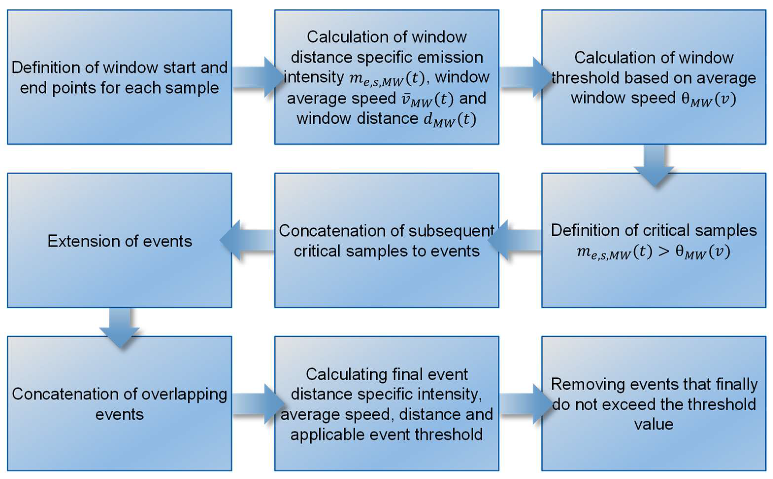
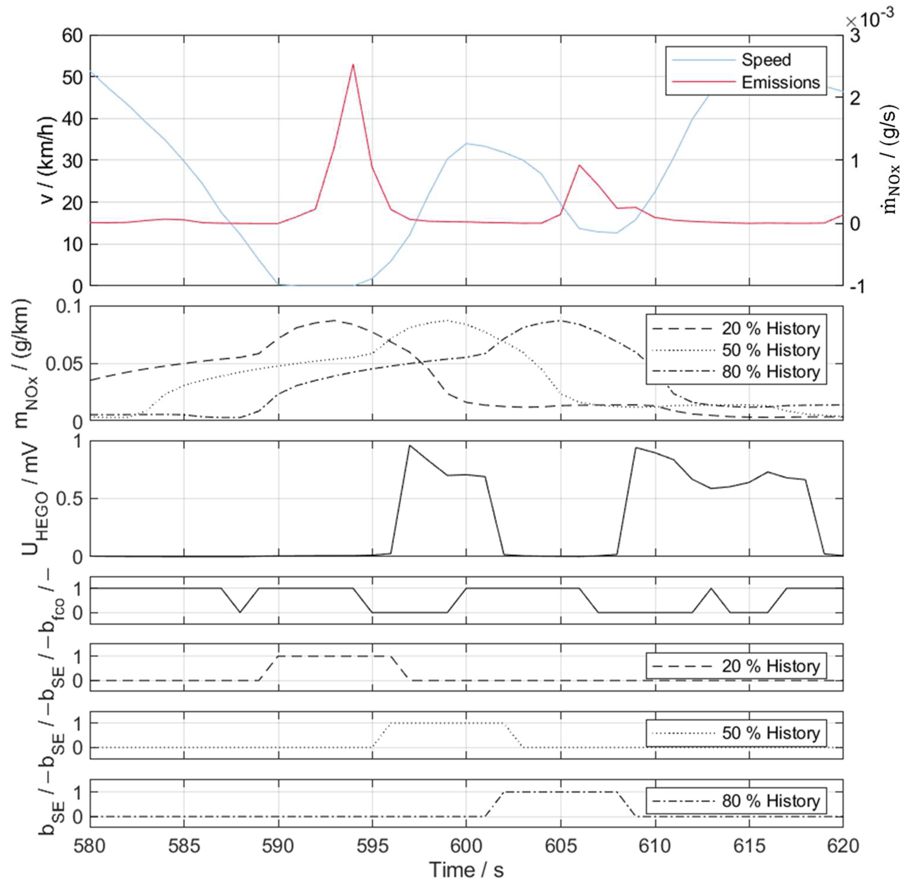
2.2. Event Detection Using Moving Window Analysis

Legislation regulates distance-specific pollutant emissions. A high value of this variable can result both from short-term emission peaks and from increased emission intensities that remain constant over a period. This is of high importance especially for low-covered distances. Therefore, for an automatic analysis of critical sequences in measurement data, two different approaches can be chosen:

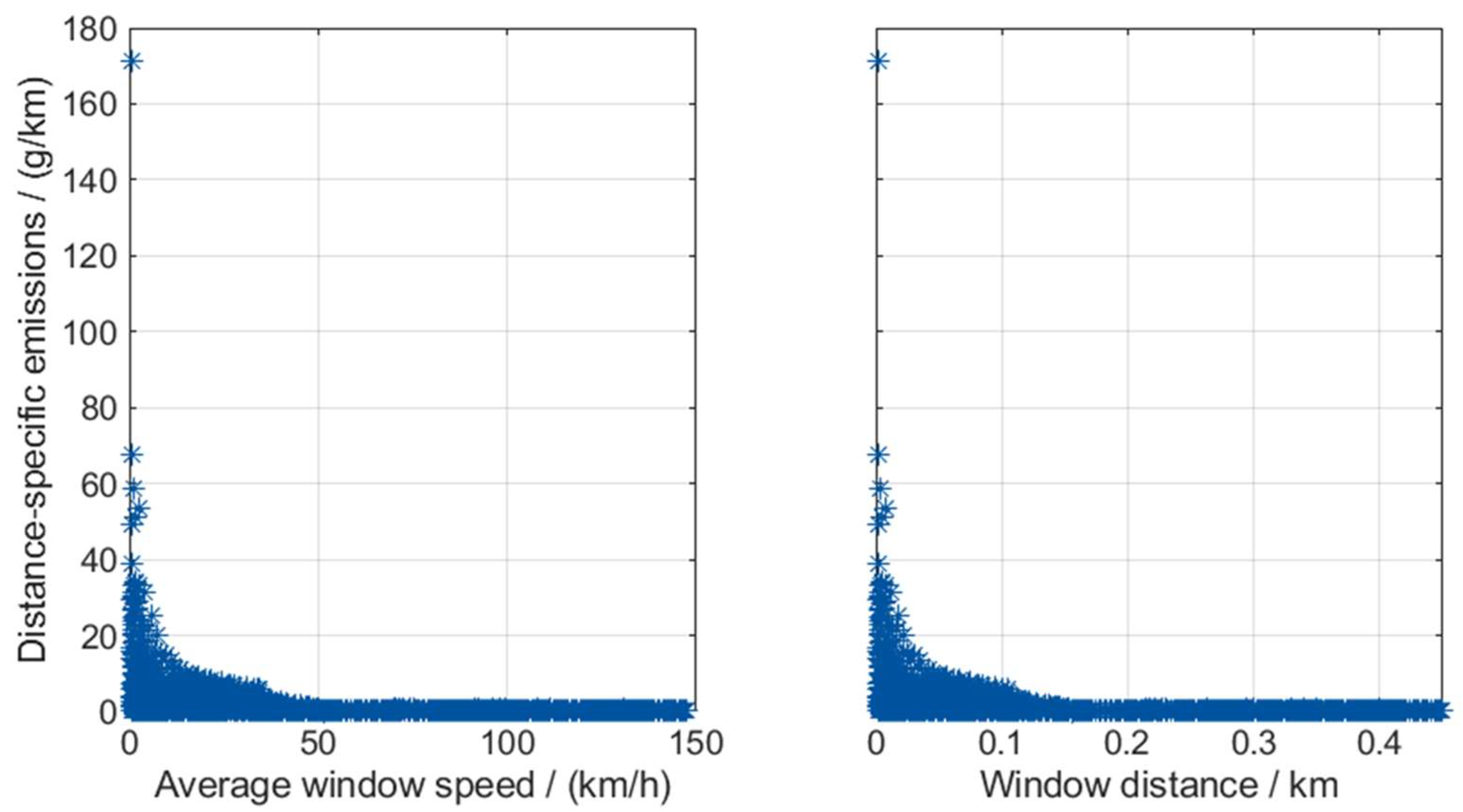
• Peaks can be identified on a time basis by directly comparing the measured value with a threshold value or by determining the deviation from an (moving) average value.
• Phases of increased emissions can be identified by their distance-specific course.

The definition of the threshold intensity in a time-based detection method is highly dependent on the operating point and driven speed. For high vehicle speeds, a mass flow may be uncritical; whereas, for low-speed phases, the same mass flow is highly critical. The advantage of judging the distance-specific trace is the direct consideration of the combination of emission trace and speed profile. This allows for the detection of emission events based on their impact on the overall vehicle emissions in a test. As legislative emission limits are also defined as distance-specific values, this allows to directly evaluate the intensity in comparison to these. A distance-based intensity comparison allows to decrease the direct dependency on the measurement system that could lead to different characteristics of volume or mass flow peaks based on the sensor position and gas flow time when considering a higher distance than provided by a single sample. A similar advantage could be achieved by time-based methods by using, e.g., moving average windows.

Therefore, a distance-specific approach is applied in the procedure described here. Alternatives, such as peak detections and time-based threshold-exceeding detections or gradient-based strategies, have initially been analyzed for the specific use-case but resulted in a high dependency of vehicle and drive profile. Approaches for such can be for example found in [46]. Further methods for detecting events in time-based signals may use outlier detections as given in an overview in [47,48]. Besides this, pattern recognition methods may be useful for event detection algorithms to either identify repeating patterns or discords in measurement traces as discussed, e.g., in [49]. Contrary to the recognition of outliers or discords as well as the identification of repeating patterns, for example, generically applicable with the matrix profile approach presented in [50,51], the shape and repeatability of critical sequences are not of interest specifically. Here, in the first step, the only relevant characteristic is the increased emission intensity. Therefore, the use of such approaches is waived, and a distance-specific threshold analysis is performed.

In both time-specific and distance-specific data analysis, the evaluation of individual data points is strongly dependent on the quality of the raw data. Slight errors of the dead- and gas-time corrections of measurement systems as well as the synchronization of ECU and emission data can lead to misinterpretation of peaks of single samples. The method presented here mitigates this problem by considering defined analysis windows in which the data are evaluated like a moving average.

Time duration-defined windows of constant length (moving window—$MW$) are formed around each sample, in which the distance-specific emissions are analyzed (Equation (1)). For each sample, integral $m_{e,MW}\left(t\right)$ of the emission ($e$) vector ${\dot{m}}_e\left(t\right)$ is calculated from the beginning of the window to the end. The window is defined by the duration that is added in front of sample $∆t^{-}$ (history) and behind the sample $∆t^{+}$ (future). Similarly, the travelled distance within this time is calculated by integration of the driven speed $v\left(t\right)$.

$$m_{e,\mathrm{s},MW}\left(t\right)=\frac{m_{e,MW}\left(t\right)}{d_{MW}\left(t\right)}=\frac{{\int }_{t-∆t^{-}}^{t+∆t^{+}}{\dot{m}}_e\left(t\right)·\mathrm{d}t}{{\int }_{t-∆t^{-}}^{t+∆t^{+}}v\left(t\right)·\mathrm{d}t}$$

(1)

In this way, the calculation of the distance-specific intensity is not dependent on only one sample but is smoothed by considering a longer period. The distance-specific emission intensity $m_{e,\mathrm{s},MW}\left(t\right)$ is then compared to a threshold value for each sample. If the emissions in a window exceed the defined threshold value ${\theta }_{MW}$, the analyzed sample is considered as critical. This window procedure is similar to the MAW (moving average window) procedure used to post-process PEMS tests in comparison to their standard behavior on a WLTC (worldwide harmonized light duty test cycle). In this methodology, the CO₂ results of a WLTC are used to split the RDE measurement into windows. Each window describes a time span, in which the vehicle emits half of the CO₂ mass that is emitted during the entire WLTC [52,53]. In the procedure proposed here, the window duration follows a fixed time to reduce the dependency on the vehicle load point. Specifically for standstill and idle phases, CO₂-based windows may have an extraordinarily high duration, while for high-speed phases, the duration may be rather short. At the same time, a direct correlation between pollutants like PN or NO_X to the CO₂ emission cannot be assumed in general. While the CO₂ emission mainly reflects the required load and power (in combination with the efficiency, the fuel consumption), the formation of pollutants is assumed to be rather situation- and drive-profile-dependent.

The duration of the windows is particularly decisive for the intensity of the emission profile for each sample and with this for the length of critical segments. Different lengths are suitable for detecting both long-term elevated emission sequences and short-term peaks. The distribution of window lengths around the analysis point defines at which point in time a critical event is detected. By shifting the center of the window away from the sample ($∆t^{+}\ne ∆t^{-}$), the recording flag for critical sequences is set at times where the actual emission intensity may not yet be critical (e.g., for high $∆t^{+}$ values). The subsequent analysis of the root causes for the emission intensities is based on the actual time-based profile and thus not influenced by this.

The windows are characterized by different durations $∆t_{MW}$. In the analysis here, an iteration of durations and combinations of history and future shares is performed. The effect of different combinations of the overall window durations and shares of considered history and future will be discussed in Section 3.

The overall principle of the event detection procedure is visualized in Figure 2. Following the calculation of all windows’ start and end positions, the window results are calculated for each sample. For each sample, several windows of different durations are created. Afterwards, the window-specific threshold is calculated for each sample. By comparing the window intensity to the threshold, the sample is categorized into critical or uncritical. Consecutive critical samples are concatenated to a raw event. These are extended in their history ($+5 \mathrm{s})$ and future ($+2 \mathrm{s}$) to further reduce the dependency on exact data synchronization and to allow a higher consideration of the events’ history. To optimize the detection to typical gasoline engine weak spots, events starting with a low downstream lambda sensor voltage ($U_{\mathrm{H}\mathrm{E}\mathrm{G}\mathrm{O}}<500\mathrm{m}\mathrm{V}$—indicating a high amount of oxygen in the three-way catalytic converter) or an activated fuel cut-off state are further extended in their history to the beginning of the critical state and a maximum of $7 \mathrm{s}$. Events that overlap each other after this correction are merged to a single event. For each of the final events, the distance-specific emission intensity, travelled distance and average speed are calculated. Events with a travelled distance of less then $5 \mathrm{m}$ are removed. For each event, the applicable threshold value is again calculated based on the final event’s average speed. Events that are not exceeding the threshold value anymore are also removed.

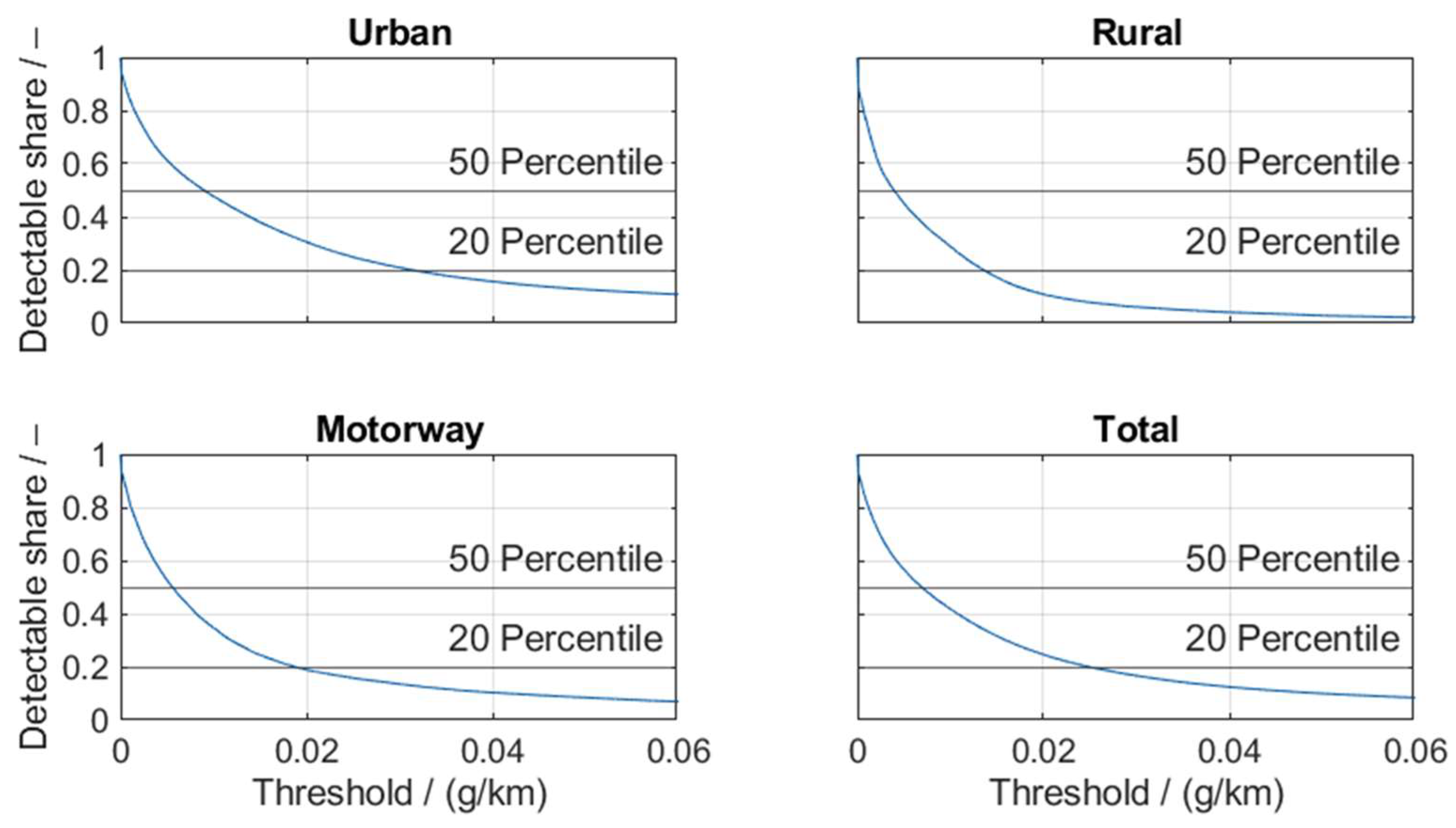
2.3. Detection Threshold

The level of the threshold depends on the desired intensity and is system-specific. Setting high threshold values (greater than or equal to the legal limit) is suitable for creating emission-critical cycles. The generation of a relevant driving profile although requires a sufficiently large number of identifiable events, which depends on the baseline emission intensity of the vehicle. Selecting a threshold value that is too high for the vehicle results in only a small number of emission events being detected. A threshold value that is too low results in a permanent detection of the static baseline emissions.

To define the specific threshold, an algorithm is created that first calculates the travelled window distance $d_{MW}\left(t\right)$, the average window speed ${\overline{v}}_{MW}\left(t\right)$ and the integrated window emissions $m_{e,MW}\left(t\right),$ according to Equation (1). Here, the window is arranged symmetrically around every sample using a window setting of $∆t^{-}=∆t^{+}=5 \mathrm{s}$. Afterwards, all samples that show a window distance of $d_{MW}\left(t\right)<0.002 \mathrm{k}\mathrm{m}$, negative cumulated emission intensities $m_{e,MW}\left(t\right)<0$ or $NaN$ values due to measurement errors are removed. Then, the distance-specific window emission intensity $m_{e,\mathrm{s},MW}\left(t\right)$ is calculated (Equation (1)). The window intensities are shown in Figure 3 based on the average window speed (left) and window distance (right). The data show an overall lower intensity with increasing window speeds due to the higher travelled distance. This motivates for a threshold value that is more dependent on the vehicle speed than a static value.

Figure 3. NO_X emission intensity based on average speed and distance for threshold analysis.To define the threshold as a speed-dependent value, an investigation of the impact of a potential threshold value is performed for each RDE phase. According to the legislation [4], the urban phase $\mathrm{u}$ is defined by $0\frac{\mathrm{k}\mathrm{m}}{\mathrm{h}}\le v\le 60\frac{\mathrm{k}\mathrm{m}}{\mathrm{h}}$, rural $\mathrm{r}$ by $60\frac{\mathrm{k}\mathrm{m}}{\mathrm{h}}<v\le 90\frac{\mathrm{k}\mathrm{m}}{\mathrm{h}}$ and motorway $\mathrm{m}$ is defined as $90\frac{\mathrm{k}\mathrm{m}}{\mathrm{h}}<v$. For the motorway phase, the maximum limit of $160\frac{\mathrm{k}\mathrm{m}}{\mathrm{h}}$ is not considered, to also take higher speeds into consideration during the calibration process. The share of detectable samples for potential threshold values is shown in Figure 4.

Figure 3. NO_X emission intensity based on average speed and distance for threshold analysis.To define the threshold as a speed-dependent value, an investigation of the impact of a potential threshold value is performed for each RDE phase. According to the legislation [4], the urban phase $\mathrm{u}$ is defined by $0\frac{\mathrm{k}\mathrm{m}}{\mathrm{h}}\le v\le 60\frac{\mathrm{k}\mathrm{m}}{\mathrm{h}}$, rural $\mathrm{r}$ by $60\frac{\mathrm{k}\mathrm{m}}{\mathrm{h}}<v\le 90\frac{\mathrm{k}\mathrm{m}}{\mathrm{h}}$ and motorway $\mathrm{m}$ is defined as $90\frac{\mathrm{k}\mathrm{m}}{\mathrm{h}}<v$. For the motorway phase, the maximum limit of $160\frac{\mathrm{k}\mathrm{m}}{\mathrm{h}}$ is not considered, to also take higher speeds into consideration during the calibration process. The share of detectable samples for potential threshold values is shown in Figure 4.

Figure 4. Impact of potential threshold values on the share of detectable critical samples.

Figure 4. Impact of potential threshold values on the share of detectable critical samples.

Here, the integrated NO_X window emissions are compared to the threshold on the x-axis. If the window emissions are exceeding the threshold, they are counted as detectable. The y-axis demonstrates how many single samples (relative to the absolute number of samples in the specific RDE phase) can be identified as critical for a certain threshold value. For the later event detection, it must be considered that a final event is defined by a series of critical samples. The final threshold is usually defined by a value between the 20th percentile and the 50th percentile to be able to detect a suitable number of events for system optimization.

Comparing the impacts for urban (top left), rural (top right), motorway (bottom left) and total (bottom right), the difference in the baseline level of the different speed phases becomes visible. While for the urban phase, a value up to roughly $30\frac{\mathrm{m}\mathrm{g}}{\mathrm{k}\mathrm{m}}$ (reflecting $50\%$ of the legislative NO_X limit) reflects the 20th percentile, such a value would not allow to identify a sufficient number of events for rural and motorway areas. For the rural area, a lower threshold is suggested than for the motorway phase. This is often caused by events in the motorway phase that show too high of space velocities due to high exhaust gas mass flow at high-speed accelerations, leading to an insufficient conversion in the catalytic converter.

The threshold for each sample’s moving window is based on the average speed within the window. The threshold is designed as a linear interpolation between set grid points. The linear interpolation focuses on the physical system behavior and avoids sudden changes in the threshold value, which would occur with fixed threshold limits for the RDE phases urban, rural and motorway (switch instead of interpolation). In the calculation according to Equation (2), the threshold value for a corresponding window ${\theta }_{MW}$ is determined by the emission threshold ${\mathsf{\theta }}_{\mathrm{u},\mathrm{r},\mathrm{m}}$ and the velocity points ${\mathrm{v}}_{\mathsf{\theta },\mathrm{u},\mathrm{r},\mathrm{m}}$ based on the average velocity of the window ${\overline{v}}_{MW}$.

$${\theta }_{MW}({\overline{v}}_{MW})=\left\{\begin{array}{ll}{\mathsf{\theta }}_{\mathrm{u}}& ,{\overline{v}}_{MW}\le {\mathrm{v}}_{\mathsf{\theta },\mathrm{u}}\\ {\mathsf{\theta }}_{\mathrm{u}}+\frac{{\overline{v}}_{MW}-{\mathrm{v}}_{\mathsf{\theta },\mathrm{u}}}{{\mathrm{v}}_{\mathsf{\theta },\mathrm{r}}-{\mathrm{v}}_{\mathsf{\theta },\mathrm{u}}}·\left({\mathsf{\theta }}_{\mathrm{r}}-{\mathsf{\theta }}_{\mathrm{u}}\right)& , {\mathrm{v}}_{\mathsf{\theta },\mathrm{u}}<{\overline{v}}_{MW}\le {\mathrm{v}}_{\mathsf{\theta },\mathrm{r}}\\ {\mathsf{\theta }}_{\mathrm{r}}+\frac{{\overline{v}}_{MW}-{\mathrm{v}}_{\mathsf{\theta },\mathrm{r}}}{{\mathrm{v}}_{\mathsf{\theta },\mathrm{m}}-{\mathrm{v}}_{\mathsf{\theta },\mathrm{r}}}·\left({\mathsf{\theta }}_{\mathrm{m}}-{\mathsf{\theta }}_{\mathrm{r}}\right)& ,{\mathrm{v}}_{\mathsf{\theta },\mathrm{r}}<{\overline{v}}_{MW}\le {\mathrm{v}}_{\mathsf{\theta },\mathrm{m}}\\ {\mathsf{\theta }}_{\mathrm{m}}& , {\mathrm{v}}_{\mathsf{\theta },\mathrm{m}}<{\overline{v}}_{MW}\end{array}\right.$$

(2)

Within the here-discussed exemplary application of the event detection, the values are set according to

Table 1. Applied threshold values for event detection.

Criteria	$\mathbf{Urban} \mathbf{u}$	$\mathbf{Rural} \mathbf{r}$	$\mathbf{Motorway} \mathbf{m}$
${\mathrm{v}}_{\mathsf{\theta },i}$/$\left[\frac{\mathrm{k}\mathrm{m}}{\mathrm{h}}\right]$	$50$	$75$	$120$
${\mathsf{\theta }}_i$/[$\frac{\mathrm{m}\mathrm{g}}{\mathrm{k}\mathrm{m}}$]	$60$	$30$	$30$

, reflecting roughly the tenth percentile of detectable samples using the $\pm 5 \mathrm{s}$ windows.

While a higher number of events based on the 20th percentile is usually preferred for the calibration process, the lower number is chosen here to evaluate the algorithm of event detection itself. A detailed judgement of the vehicle’s calibration is not targeted.

2.4. Test Parameters and Data

The analysis of the event detection is carried out in three steps:

• The basic setup of the event detection is implemented.
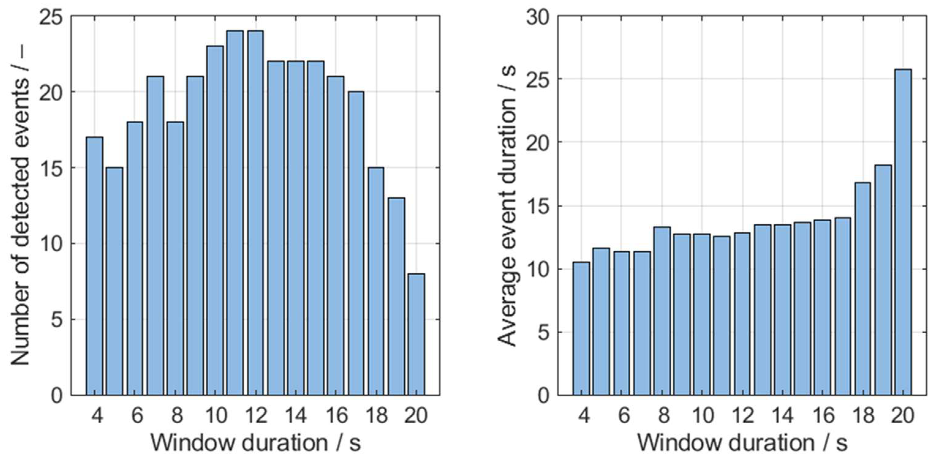
• The duration of the windows is varied to analyze the impact of the timespan that can be considered for each sample.
• The layout of the windows around each sample is modified to investigate the influence of different distributions of history and future shares.

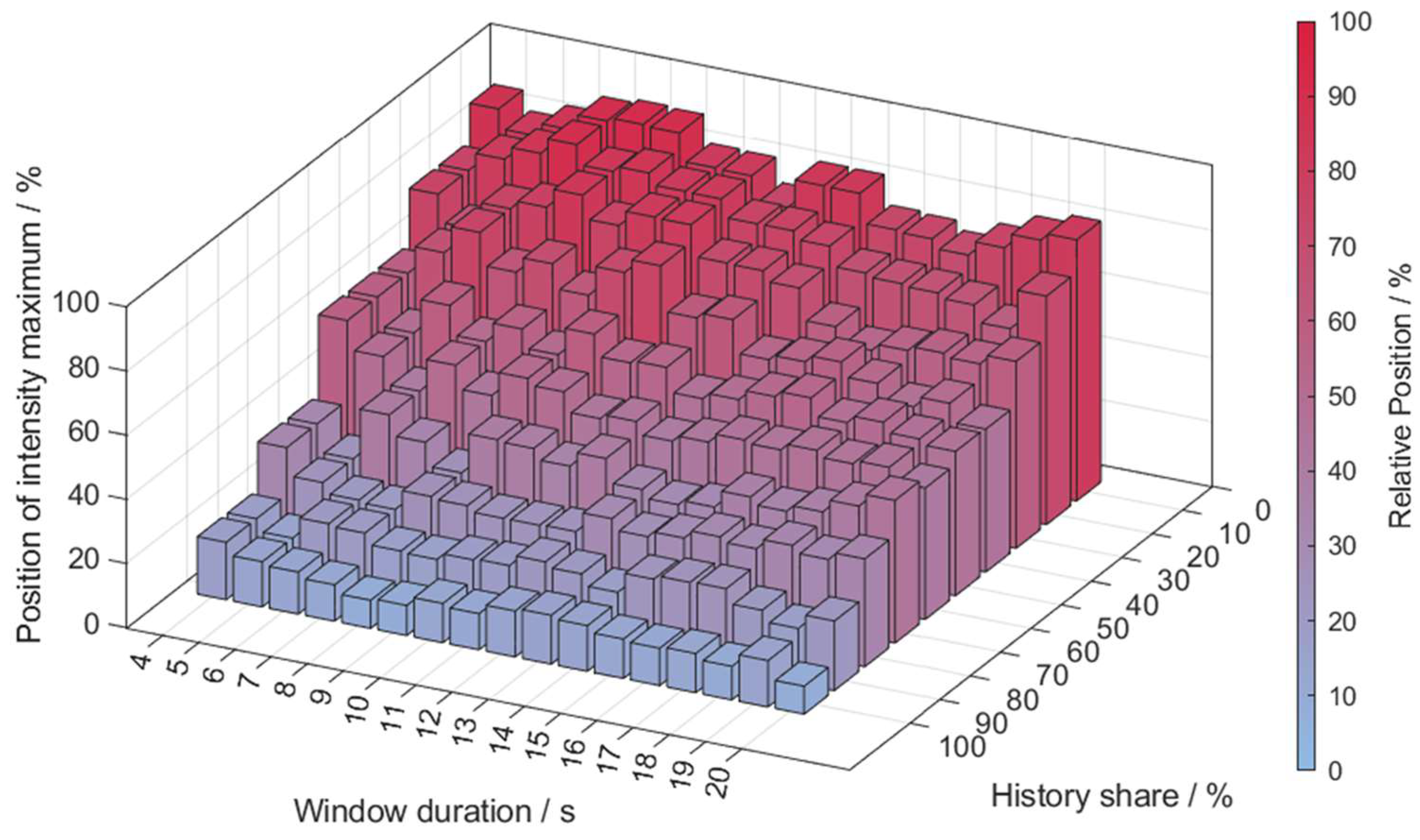
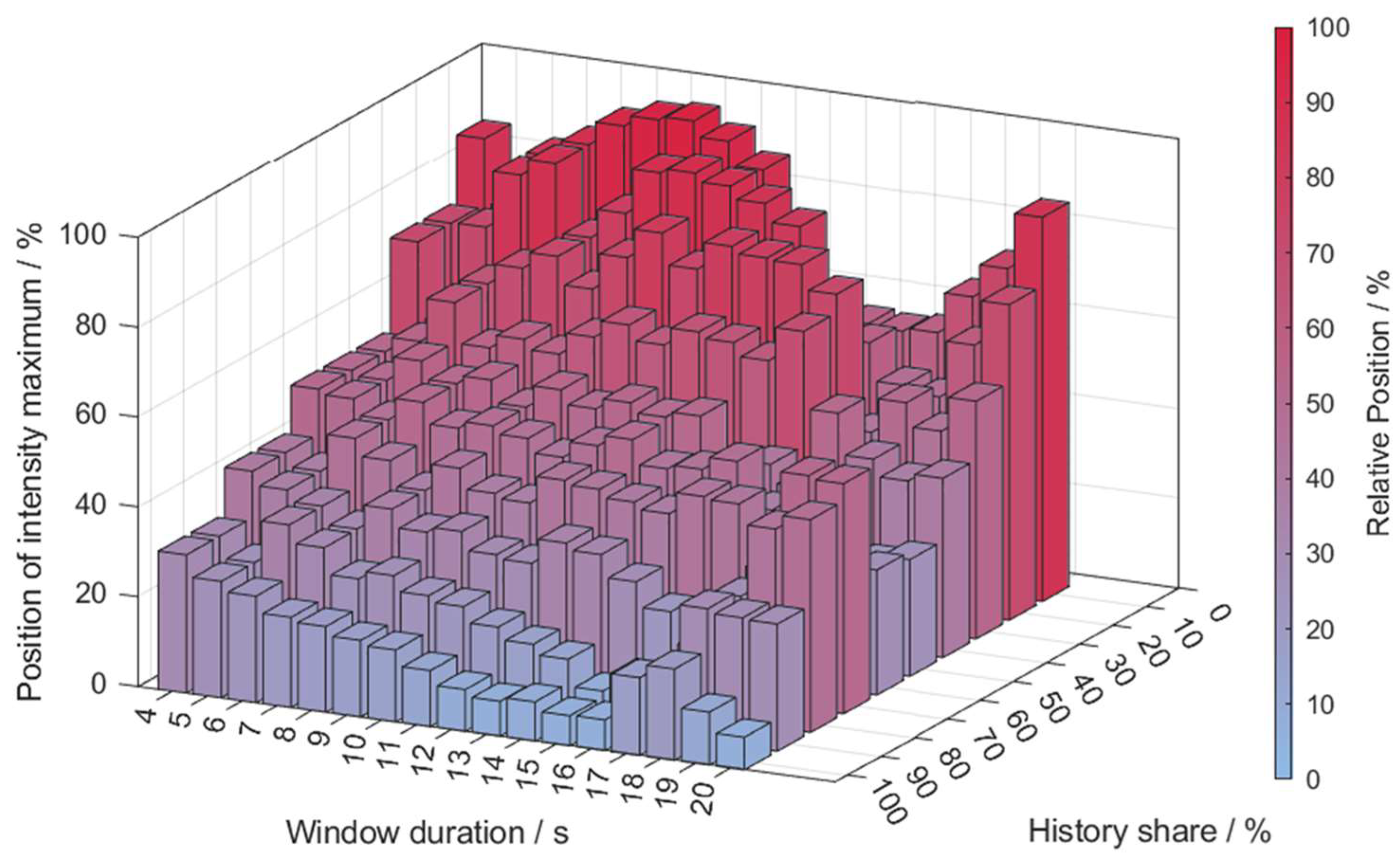
The database consists of $60$ emission measurements carried out during the development process of a gasoline engine-powered vehicle. It includes $13$ PEMS measurements of different routes and $47$ chassis dynamometer tests using $12$ different speed profiles at varying ambient conditions. The ECU dataset as well as vehicle hardware are kept constant within all measurements and are designed for EU6d legislation. The data were collected with a J segment vehicle, as described in

Table 2. Specifications of test vehicle.

Criteria	Value	Criteria	Value
Vehicle mass	$>2000 \mathrm{k}\mathrm{g}$	Drivetrain	All-wheel drive (AWD)
Engine	Inline 4 cylinder	Gearbox	Automatic Transmission (AT)
Max. power	$>180 \mathrm{k}\mathrm{W}$	EATS	Three-way catalytic converter (TWC) and Gasoline particulate filter (GPF)
Max. torque	$>300 \mathrm{N}\mathrm{m}$	Fuel	Gasoline

.

For the window layout, different durations are calculated iteratively with window durations from $4 \mathrm{s}$ up to $20 \mathrm{s}$ with a step size of $1 \mathrm{s}$. The positioning of the windows around each sample is also adjusted iteratively for each window duration considering $0\%$ to $100\%$ of the window duration in the past of the sample with a step size of $10\%$. To test the behavior of the event detection on different characteristics of target data, it is applied to the trace of the NO_X tailpipe emission mass flow and to the trace of PN tailpipe emission number flow. All data are resampled to an $f=1 \mathrm{H}\mathrm{z}$ resolution to provide the same resolution of PEMS measurement data (available in $f=1 \mathrm{H}\mathrm{z}$), chassis dynamometer data (available in $f=10 \mathrm{H}\mathrm{z}$) and ECU data (recorded by integrated calibration and application tool software INCA(V7.3) by ETAS in different, higher frequencies).

3. Results

The influence of different window lengths on the number of detected events and their average duration are shown for PN emissions in Figure 5 and for NO_X emissions in Figure 6. For the definition of critical sequences, the data from Table 1 are applied. For the PN events, the number of detected events (Figure 5, left) decreases with increasing window length. At the same time, the average duration of the detected events increases (Figure 5, right). A similar pattern for the duration of the detected events is shown for NO_X emissions (Figure 6, right).

Contrary to the trend of decreasing event number with increasing window length for PN emissions, NO_X emissions show a maximum at $12 \mathrm{s}$ window duration. This trend is due to the varying threshold over the velocity. By lengthening the windows, a lower average speed is achieved in some cases than in the shorter windows. This correspondingly increases the relevant threshold. In addition, the events in longer windows are partly interrupted and can be divided into several individual events.

A qualitative weak spot analysis and the reproduction of critical sequences on a test bench require a detection period that contains the root cause of the event. Detecting events just once the critical intensity is present will not allow to reproduce the critical system behavior or analysis. A criterion to judge the positioning of the windows is the location of the intensity maximum within the events. To enable a reproduction of the causal system states, the detection of the event before reaching the maximum intensity is useful. The effect of window length and distribution of duration around the analysis point on the position of the intensity maximum is shown for PN in Figure 7 and for NO_X in Figure 8.

For different window durations ($∆t_{MW}=4 \mathrm{s}$ to $∆t_{MW}=20 \mathrm{s}$), the intensity maximum position is evaluated for history ($∆t^{-}$) shares of $∆t_{\mathrm{s}}^{-}=0\%$ (analyzing only future of sample—looking forward) to $∆t_{\mathrm{s}}^{-}=100\%$ (analyzing only history of sample—looking backward) in $10\%$ steps. A full-history consideration ($∆t_{\mathrm{s}}^{-}=100\%$) will calculate the sample intensity based on the last $∆t_{MW}$ seconds. Therefore, it only considers data that already happened. The events displayed here are formed by concatenating consecutive critical samples (event duration not limited by window duration). The analyzed relative maximum position $i_{\mathrm{s},\mathrm{m}\mathrm{a}\mathrm{x},\mathrm{e}\mathrm{v}}\left({∆t_{MW},∆t}_{\mathrm{s}}^{-}\right)$ refers to the position in the already concanated event. The distance-specific position is evaluated relative to the length of the event. A value of $i_{\mathrm{s},\mathrm{m}\mathrm{a}\mathrm{x},\mathrm{e}\mathrm{v}}=0\%$ means that the distance-specific intensity maximum occurs directly at the beginning of the recording. For a value of $i_{\mathrm{s},\mathrm{m}\mathrm{a}\mathrm{x},\mathrm{e}\mathrm{v}}=100\%,$ the maximum is present at the end.

For PN (Figure 7), the length of the windows is not significantly relevant for the location of the maximum. The proportion of history, on the other hand, has a significant influence on its position. Across all window lengths, a decrease in the relative maximum position can be seen as the proportion of history increases. With a share of $∆t_{\mathrm{s}}^{-}=100\%$ history, an average relative position of $i_{\mathrm{s},\mathrm{m}\mathrm{a}\mathrm{x},\mathrm{e}\mathrm{v}}=10\%$ is reached, i.e., a position in the event immediately after the start of recording. Considering $∆t_{\mathrm{s}}^{-}=0\%$ history, the maximum occurs significantly later in the recorded sequence at $i_{\mathrm{s},\mathrm{m}\mathrm{a}\mathrm{x},\mathrm{e}\mathrm{v}}=80\%$.

The consideration of the influence of $∆t_{MW}$ and share of history $∆t_{\mathrm{s}}^{-}$ for NO_X (Figure 8) shows slight differences. With a low proportion of history, increased fluctuations of the position depending on the window duration occur. A maximum of about $i_{\mathrm{s},\mathrm{m}\mathrm{a}\mathrm{x},\mathrm{e}\mathrm{v}}=90\%$ is reached with a window duration of $∆t_{MW}=10 \mathrm{s}$ and a history share of $∆t_{\mathrm{s}}^{-}=10\%$. Analogous to the behavior for PN, the influence of history on the position of the maximum also predominates for NO_X emissions. A decreasing trend of the relative position with increasing share of history can be derived. However, the latest position is not detected at the lowest share of history, especially in the range of window lengths between $∆t_{MW}=13 \mathrm{s}$ and $∆t_{MW}=17 \mathrm{s}$, but reaches this point at a share of history of about $∆t_{\mathrm{s}}^{-}=20\%$ to $∆t_{\mathrm{s}}^{-}=30\%$.

The influence of the history portion on recorded sequence and the position of the intensity maximum is illustrated in Figure 9. For a measurement section with NO_X emissions, the effect of three different history distributions for event detection with $∆t_{MW}=20 \mathrm{s}$ window duration is shown. In addition to the velocity $v$, NO_X emission mass flow ${\dot{m}}_{\mathrm{N}\mathrm{O}\mathrm{x}}$, voltage of downstream lambda sensor $U_{\mathrm{H}\mathrm{E}\mathrm{G}\mathrm{O}}$ and the indicator for the presence of operation in fuel cut-off $b_{\mathrm{f}\mathrm{c}\mathrm{o}}$, the distance-specific emission intensities $m_{\mathrm{N}\mathrm{O}\mathrm{x}}$ for the three window variations are shown. The last three plots show the time during which the emission threshold is exceeded $b_{\mathrm{S}\mathrm{E}}$ (bit single event).

In the deceleration phase at the start of the event ($t=580 \mathrm{s}$ to $t=590 \mathrm{s}$), the vehicle is in fuel cut-off mode, in which no fuel is injected into the cylinders. As a result, the catalytic converter is saturated with oxygen. The condition is expressed by the low lambda sensor voltage. Thus, the system is not capable of sufficiently converting NO_X emissions during restart ($t=594 \mathrm{s}$), resulting in the increased NO_X intensity. Due to the rich mixture used to purge the catalytic converter, the stored oxygen decreases, which is evident from the increasing $U_{\mathrm{H}\mathrm{E}\mathrm{G}\mathrm{O}}$ ($t=597 \mathrm{s}$). The subsequent renewed braking phase with fuel cut-off ($t=600 \mathrm{s}$ to $t=607 \mathrm{s}$) again leads to a state of insufficient conversion efficiency and thus to a further breakthrough of NO_X emissions, which remains uncritical in its intensity ($t=607 \mathrm{s}$ to $t=615 \mathrm{s}$).

Comparing the detection of critical intensities during restart in the different window layouts, the window with $∆t_{\mathrm{s}}^{-}=50\%$ history serves as a reference, reflecting a symmetrical layout. Maximum intensity occurs shortly after the peak of the time-continuous NO_X emission mass flow, whereby the relevant threshold value is exceeded for the first time at $t=596 \mathrm{s}$ until $t=602 \mathrm{s}$. The resulting recording starts after the engine has already restarted and, although it contains the emission breakthrough itself, is not suitable for reproduction. The cause of the catalytic converter being saturated with oxygen cannot be reliably reproduced considering this period. An additional extension of the history is provided if a critical catalytic converter condition is expressed by a low sensor voltage or a fuel cut-off at the beginning of the recording. Here, there is no fuel cut-off at the start of the recording and the voltage of the lambda sensor is already rising.

If the window is split with a focus on the future and only $∆t_{\mathrm{s}}^{-}=20\%$ of the history is considered, the event is detected earlier and recording is started at the end of the braking phase. In this case, the stationary phase and the first start-up are included in the recording. Due to the extension of the history in the case of fuel cut-off and critical catalytic converter condition, the fuel cut-off phase can be reliably integrated before the event.

The variant with $∆t_{\mathrm{s}}^{-}=80\%$ history detects the same trace with a time delay and exceeds the threshold value significantly later at $t=602 \mathrm{s}$. Here, the start of the recording is in the second fuel cut-off phase, which leads to an event that is no longer critical. The actual event can, therefore, not be detected and reproduced.

Due to the different positions of the recording areas, the considered profile of emissions and system states changes accordingly. The resulting profiles for the NO_X mass flow and the distance-specific intensity in the event are shown in Figure 10 for the detection variants shown in Figure 9. The distance-specific intensity describes the quotient of the NO_X mass flow integrated up to the respective time and the distance currently traveled.

The effect on the position of the maxima becomes apparent. For the window with $∆t_{\mathrm{s}}^{-}=20\%$ history (Figure 10, top), the event is detected early. As a result, the peak of the mass flow as well as distance-specific intensity is at the end of the recording. This results in a high relative share of the event to be available for conditioning the system toward the critical state. Although the time-continuous maximum is reached after the end of this event and is correspondingly early in the variant with $∆t_{\mathrm{s}}^{-}=50\%$ history (Figure 10 center), the core cause can be reproduced and the initial start-up can be mapped. A slight increase in the proportion of history is advisable. The distance-specific maximum is already reached at the beginning of the event at $∆t_{\mathrm{s}}^{-}=50\%$, making it difficult to reproduce the system state. The progression of the $∆t_{\mathrm{s}}^{-}=80\%$ history variant (Figure 10, bottom) shows a consistently non-critical emission progression since the critical sequence has already been passed.

4. Discussion

With the investigated approach for event detection in emission calibration, a high potential to automatically analyze a high amount of data for relevant sequences is seen. Judging sequences with a distance-specific approach offers a way to detect critical sequences caused by low travelled distance as well as sequences characterized by high emission intensity. Although the scanning approach of the moving analyzing windows smoothens out the measurement quality for each sample, a high dependency on the explicit layout is seen. On the one hand, the overall duration of the window that is used to evaluate the distance-specific intensity for each sample is influencing the estimation. On the other hand, the layout around each sample is a crucial factor.

Windows of higher durations examine longer driving sections. This reduces the number of detected events in general, although it also changes the average speed of the window that decides on the applied threshold. While long window durations consider primarily long-term increased emission intensities, short durations are useful to detect peak events. After the single samples are analyzed by windows, the final events are re-evaluated. For each event as combination of consecutive critical samples, the average speed and distance-specific emission intensity for the complete event is calculated and compared to a final threshold. Here, the average speed of the event can deviate from the average speed that was considered for each single sample, which causes the threshold value to change. To reduce the difference in average speed (and thus, threshold value) between the samples and the final overall event, it is suggested to use multiple windows at the same time.

For the final layout of the windows around each sample, the target of root cause analysis and reproducibility when re-driving the events is to be considered. The extracted events must be detected already slightly before the critical intensity is evident to include the recording of the operation that has led to the critical system state. A high focus on the future development of emissions leads to the detection of driving events in which there is not yet an increased intensity. A strong consideration of the past and symmetrical layouts lead to emission events being detected too late. As a result, the emissions in the marked area flatten out already and the recording of the origin of the event is lost.

With the findings on the influence of length and history, different windows are used simultaneously in the project application, which enables the detection of both short-term critical and long-term intensive driving situations. With extension in case of occurring fuel cut-off phases or critical catalytic converter states at the beginning of the event, a distribution of $25\%$ history and $75\%$ future is suitable to detect sequences that still show a critical intensity but also show the operating conditions that lead to these.

Table 3. Overview of event detection window layout.

Type	$\mathsf{\Delta }{\mathit{t}}^{\mathbf{t}\mathbf{o}\mathbf{t}\mathbf{a}\mathbf{l}}$	$\mathsf{\Delta }{\mathit{t}}^{-}$	$\mathsf{\Delta }{\mathit{t}}^{+}$
${\mathrm{M}\mathrm{W}}_{\mathrm{p}\mathrm{e}\mathrm{a}\mathrm{k}}$	$4$	$1$	$3$
${\mathrm{M}\mathrm{W}}_{\mathrm{s}\mathrm{h}\mathrm{o}\mathrm{r}\mathrm{t}}$	$10$	$2$	$8$
${\mathrm{M}\mathrm{W}}_{\mathrm{m}\mathrm{e}\mathrm{d}\mathrm{i}\mathrm{u}\mathrm{m}}$	$16$	$4$	$12$
${\mathrm{M}\mathrm{W}}_{\mathrm{l}\mathrm{o}\mathrm{n}\mathrm{g}}$	$20$	$5$	$15$

shows the finally selected layouts.

Using these settings, a total amount of 454 events can be identified from 60 measurements. This reduces the overall $\mathrm{184,623} \mathrm{s}$ of measurements to a relevant amount of $\mathrm{12,823} \mathrm{s}$. With the events showing an average duration of $28 \mathrm{s}$, they can be further clustered as described in [54] to reduce the manual effort for the analysis of weak spots.

The moving analyzing windows around each sample of a measurement make the analysis methodology robust against slight errors in the signal. The design of the windows with an asymmetric distribution around the analysis point allows the measurement data to be examined with a focus on future signal development. Thus, critical sequences are already marked in their origin before the actual emission intensity exceeds the defined threshold. This approach helps to understand the cause of the critical behavior and allows the reproduction of the critical sequence in later emission tests.

5. Conclusions

The current EU6d legislation sets the boundary conditions for vehicle emission validation, while the potential extension of EU7 legislation further expands the scope for testing a wide range of scenarios in automotive engineering. During the development process, a variety of tests are performed on the chassis dynamometer with different speed profiles and on the open road with PEMS in different boundary conditions. To minimize the level of manual analysis for identifying weak spots in a large amount of measurement data, this article proposes an event detection approach that is capable of automatically examining all accessible data and narrowing it down to the areas that require manual analysis. The method is independently from advanced access to ECU values and solely relies on emission and speed signals.

Detection of critical sequences involves

• Definition of analysis windows for each measurement sample with focus into the future development of the signal traces.
• Integration of emission intensity and driven distance within these windows for calculation of distance-specific emission intensity for each sample.
• Threshold identification for critical intensity based on the average speed within the analysis windows for each sample.
• Comparison of the distance-specific intensity to the threshold for each sample and marking of critical samples.
• Summarizing consecutive critical samples to an event.
• Extension of beginning of event into past in case of critical initial situation (e.g., fuel cut-off).
• Re-check of final event duration for critical intensity.

Parameters such as the speed-dependent threshold, number of windows per sample, duration of windows and positioning distribution of windows can be adjusted for vehicle individual use. The initial presented methodology for the threshold identification is crucial for detecting vehicle-specific weak points and preventing critical data from being undetected due to a selected threshold value that is set too high or for identifying long-lasting events in the basic emission level. For the design of window duration, the impact analysis suggests using multiple windows with different durations. For the distribution of windows around the measurement samples, the analysis suggests a trend of focusing the analysis windows slightly into the future instead of symmetrically around the sample. This shows the advantage of identifying critical samples with a sufficient share of history to understand and reproduce the critical system behavior. At the same time, this leads to the approach of not being directly real-time capable, as a share of the future signal traces must be known. While the event detection is only applied after having collected complete measurements here, it could as well be applied in real-time with a slight delay of the required future share of the designed windows.

Additionally, it is being studied for its application in other technical fields of vehicle development. Battery electric vehicles are a particular area of focus where the methodology can provide support for, e.g., thermal management. In addition, the combination with fuel cell calibration tasks and the investigation of aging effects for fuel cell systems is focused. The topic of analyzing the optimization of vehicle operation strategies in hybrid vehicles is currently being investigated to improve system efficiency.

References

1. European Commission. The European Green Deal: Communication from the Commission to the European Parliament, the European Council, the Council, the European Economic and Social Committee and the Committee of the Regions; 640 Final; Official Journal of the European Union: Brussels, Belgium, 2019.
2. Mulholland, E.; Miller, J.; Braun, C.; Jin, L.; Rodriguez, F. Quantifying the Long-Term Air Quality and Health Benefits from Euro 7/VII Standards in Europe. Available online: https://euagenda.eu/upload/publications/eu-euro7-standards-health-benefits-jun21.pdf (accessed on 3 January 2024).
3. Mulholland, E.; Miller, J.; Bernard, Y.; Lee, K.; Rodríguez, F. The role of NOx emission reductions in Euro 7/VII vehicle emission standards to reduce adverse health impacts in the EU27 through 2050. Transp. Eng. 2022, 9, 100133. [Google Scholar] [CrossRef]
4. European Parliament and Council. Commission Regulation (EU) 2018/1832; Official Journal of the European Union: Brussels, Belgium, 2018. [Google Scholar]
5. European Commission. Commission Regulation (EU) 2017/1151; Official Journal of the European Union: Brussels, Belgium, 2017.
6. European Commission. Proposal for a Regulation of the European Parliament and of the Council on Type-Approval of Motor Vehicles and Engines and of Systems, Components and Separate Technical Units Intended for Such Vehicles, with Respect to Their Emissions and Battery Durability (Euro 7) and Repealing Regulations (EC) No 715/2007 and (EC) No 595/2009; Official Journal of the European Union: Brussels, Belgium, 2022; Volume 0365.
7. Boger, T.; Rose, D.; He, S.; Joshi, A. Developments for future EU7 regulations and the path to zero impact emissions—A catalyst substrate and filter supplier’s perspective. Transp. Eng. 2022, 10, 100129. [Google Scholar] [CrossRef]
8. Giechaskiel, B.; Bonnel, P.; Perujo, A.; Dilara, P. Solid Particle Number (SPN) Portable Emissions Measurement Systems (PEMS) in the European Legislation: A Review. Int. J. Environ. Res. Public Health 2019, 16, 4819. [Google Scholar] [CrossRef] [PubMed]
9. Giechaskiel, B.; Clairotte, M.; Valverde, V.; Bonnel, P. Real Driving Emissions: 2017 Assessment of PEMS Measurement Uncertainty; Publications Office of the European Union: Luxembourg, 2017. [Google Scholar] [CrossRef]
10. Giechaskiel, B.; Lähde, T.; Gandi, S.; Keller, S.; Kreutziger, P.; Mamakos, A. Assessment of 10-nm Particle Number (PN) Portable Emissions Measurement Systems (PEMS) for Future Regulations. Int. J. Environ. Res. Public Health 2020, 17, 3878. [Google Scholar] [CrossRef] [PubMed]
11. Giechaskiel, B.; Casadei, S.; Mazzini, M.; Sammarco, M.; Montabone, G.; Tonelli, R.; Deana, M.; Costi, G.; Di Tanno, F.; Prati, M.; et al. Inter-Laboratory Correlation Exercise with Portable Emissions Measurement Systems (PEMS) on Chassis Dynamometers. Appl. Sci. 2018, 8, 2275. [Google Scholar] [CrossRef]
12. Varella, R.; Giechaskiel, B.; Sousa, L.; Duarte, G. Comparison of Portable Emissions Measurement Systems (PEMS) with Laboratory Grade Equipment. Appl. Sci. 2018, 8, 1633. [Google Scholar] [CrossRef]
13. Czerwinski, J.; Zimmerli, Y.; Hüssy, A.; Engelmann, D.; Bonsack, P.; Remmele, E.; Huber, G. Testing and evaluating real driving emissions with PEMS. Combust. Engines 2018, 174, 17–25. [Google Scholar] [CrossRef]
14. Gerstenberg, J.; Hartlief, H.; Tafel, S. Introducing a Method to Evaluate RDE Demands at the Engine Test Bench; Springer Fachmedien Wiesbaden: Wiesbaden, Germany, 2016. [Google Scholar] [CrossRef]
15. Gerstenberg, J.; Hartlief, H.; Tafel, S. RDE-Entwicklungsumgebung am hochdynamischen Motorprüfstand. ATZextra 2015, 20, 36–41. [Google Scholar] [CrossRef]
16. Nies, H.; Beidl, C.; Hüners, H.; Fischer, K. Systematische Entwicklungsmethodik für Eine Robuste Motorkalibrierung unter RDE-Randbedingungen; Springer Fachmedien Wiesbaden: Wiesbaden, Germany, 2020; pp. 50–62. [Google Scholar] [CrossRef]
17. Maschmeyer, H. Systematische Bewertung Verbrennungsmotorischer Antriebssysteme Hinsichtlich Ihrer Realfahrtemissionen am Motorenprüfstand. Ph.D. Thesis, TU Darmstadt, Darmstadt, Deutschland, 2017. [Google Scholar]
18. Maschmeyer, H.; Beidl, C.; Düser, T.; Schick, B. RDE-Homologation—Herausforderungen, Lösungen und Chancen. MTZ Motortech Z 2016, 77, 84–91. [Google Scholar] [CrossRef]
19. Mayr, C.; Merl, R.; Gigerl, H.-P.; Teitzer, M.; König, D.; Stemmer, D.; Retter, F. Test emissionsrelevanter Fahrzyklen auf dem Motorprüfstand. In Simulation und Test 2018; Liebl, J., Ed.; Springer Fachmedien Wiesbaden: Wiesbaden, Germany, 2019; ISBN 978-3-658-25293-9. [Google Scholar]
20. Faubel, L.; Lensch-Franzen, C.; Schuhardt, A.; Krohn, C. Übertrag von RDE-Anforderungen in eine modellbasierte Prüfstandsumgebung. MTZ Extra 2016, 21, 44–49. [Google Scholar] [CrossRef]
21. Wasserburger, A.; Hametner, C. Automated Generation of Real Driving Emissions Compliant Drive Cycles Using Conditional Probability Modeling. In Proceedings of the 2020 IEEE Vehicle Power and Propulsion Conference (VPPC), Gijon, Spain, 18 November–16 December 2020; pp. 1–8, ISBN 978-1-7281-8959-8. [Google Scholar]
22. Wasserburger, A.; Hametner, C.; Didcock, N. Risk-averse real driving emissions optimization considering stochastic influences. Eng. Optim. 2020, 52, 122–138. [Google Scholar] [CrossRef]
23. Wasserburger, A.; Didcock, N.; Hametner, C. Efficient real driving emissions calibration of automotive powertrains under operating uncertainties. Eng. Optim. 2021, 55, 140–157. [Google Scholar] [CrossRef]
24. Donateo, T.; Giovinazzi, M. Building a cycle for Real Driving Emissions. Energy Procedia 2017, 126, 891–898. [Google Scholar] [CrossRef]
25. Dai, Z.; Niemeier, D.; Eisinger, D. Driving Cycles: A New Cycle-Bulding Method that Better Represents Real-World Emissions; University of California, Davis: Davis, CA, USA, 2008. [Google Scholar]
26. Kondaru, M.K.; Telikepalli, K.P.; Thimmalapura, S.V.; Pandey, N.K. Generating a Real World Drive Cycle–A Statistical Approach; SAE Technical Paper Series; WCX World Congress Experience; SAE International400 Commonwealth Drive: Warrendale, PA, USA, 2018. [Google Scholar]
27. Kooijman, D.G.; Balau, A.E.; Wilkins, S.; Ligterink, N.; Cuelenaere, R. WLTP Random Cycle Generator. In Proceedings of the 2015 IEEE Vehicle Power and Propulsion Conference (VPPC), Montreal, QC, Canada, 19–22 October 2015; pp. 1–6, ISBN 978-1-4673-7637-2. [Google Scholar]
28. Wu, Y.; Liu, G. Research on construction of vehicle driving cycle based on Markov chain and global K-means clustering algorithm. Veh. Dyn. 2020, 4, 1–9. [Google Scholar] [CrossRef]
29. Della Ragione, L.; Meccariello, G. Statistical approach to identify Naples city’s real driving cycle referring to the Worldwide harmonized Light duty Test Cycle (WLTC) framework. Sustain. Dev. Plan. VIII 2017, 210, 555–566. [Google Scholar] [CrossRef]
30. Balau, A.E.; Kooijman, D.; Vazquez Rodarte, I.; Ligterink, N. Stochastic Real-World Drive Cycle Generation Based on a Two Stage Markov Chain Approach. SAE Int. J. Mater. Manf. 2015, 8, 390–397. [Google Scholar] [CrossRef]
31. Roberts, P.; Mason, A.; Whelan, S.; Tabata, K.; Kondo, Y.; Kumagai, T.; Mumby, R.; Bates, L. RDE Plus—A Road to Rig Development Methodology for Whole Vehicle RDE Compliance: Overview; SAE Technical Paper Series; WCX SAE World Congress Experience; SAE International400 Commonwealth Drive: Warrendale, PA, USA, 2020. [Google Scholar]
32. Mason, A.; Roberts, P.; Whelan, S.; Kondo, Y.; Brenton, L. RDE Plus—A Road to Rig Development Methodology for Complete RDE Compliance: Road to Chassis Perspective; SAE Technical Paper Series; WCX SAE World Congress Experience; SAE International400 Commonwealth Drive: Warrendale, PA, USA, 2020. [Google Scholar]
33. Roberts, P.J.; Mumby, R.; Mason, A.; Redford-Knight, L.; Kaur, P. RDE Plus—The Development of a Road, Rig and Engine-in-the-Loop Test Methodology for Real Driving Emissions Compliance; SAE Technical Paper Series; WCX SAE World Congress Experience; SAE International400 Commonwealth Drive: Warrendale, PA, USA, 2019. [Google Scholar]
34. Andert, J.; Xia, F.; Klein, S.; Guse, D.; Savelsberg, R.; Tharmakulasingam, R.; Thewes, M.; Scharf, J. Road-to-rig-to-desktop: Virtual development using real-time engine modelling and powertrain co-simulation. Int. J. Engine Res. 2019, 20, 686–695. [Google Scholar] [CrossRef]
35. Wenig, M.; Artukovic, D.; Armbruster, C. vRDE—Virtual Real Driving Emission. In VPC—Simulation und Test 2016; Liebl, J., Beidl, C., Eds.; Springer Fachmedien Wiesbaden: Wiesbaden, Germany, 2017; ISBN 978-3-658-16753-0. [Google Scholar]
36. Riccio, A.; Monzani, F.; Landi, M. Towards a Powerful Hardware-in-the-Loop System for Virtual Calibration of an Off-Road Diesel Engine. Energies 2022, 15, 646. [Google Scholar] [CrossRef]
37. Kuznik, A.; Steinhaus, T.; Stumpp, M.; Beidl, C. Optimierung des Emissionsverhaltens innerhalb der hybriden Betriebsstrategie am Prüfstand mittels Co-Simulation. In Liebl (Hg.) 2021—Experten-Forum Powertrain; Springer: Berlin/Heidelberg, Germany, 2021; pp. 31–45. [Google Scholar] [CrossRef]
38. Donn, C.; Zulehner, W.; Pfister, F. Realfahrtests für die Antriebsentwicklung mithilfe des virtuellen Fahrversuchs. ATZ Extra 2019, 24, 44–49. [Google Scholar] [CrossRef]
39. Alilovic, M.; Corona, F.; Nica, M. Generierung eines fahrdynamikoptimierten Real-Driving-Emissions-Zyklus aus bestehenden Fahrdaten. ATZ Elektron 2022, 17, 50–54. [Google Scholar] [CrossRef]
40. Ashtari, A.; Bibeau, E.; Shahidinejad, S. Using Large Driving Record Samples and a Stochastic Approach for Real-World Driving Cycle Construction: Winnipeg Driving Cycle. Transp. Sci. 2014, 48, 170–183. [Google Scholar] [CrossRef]
41. Galgamuwa, U.; Perera, L.; Bandara, S. A Representative Driving Cycle for the Southern Expressway Compared to Existing Driving Cycles. Transp. Dev. Econ. 2016, 2, 589. [Google Scholar] [CrossRef]
42. Knopov, P.S.; Samosonok, A.S. On Markov stochastic processes with local interaction for solving some applied problems. Cybern. Syst. Anal. 2011, 47, 346–359. [Google Scholar] [CrossRef]
43. Claßen, J.; Pischinger, S.; Krysmon, S.; Sterlepper, S.; Dorscheidt, F.; Doucet, M.; Reuber, C.; Görgen, M.; Scharf, J.; Nijs, M.; et al. Statistically supported real driving emission calibration: Using cycle generation to provide vehicle-specific and statistically representative test scenarios for Euro 7. Int. J. Engine Res. 2020, 21, 1783–1799. [Google Scholar] [CrossRef]
44. Claßen, J. Entwicklung Statistisch Relevanter Prüfszenarien zur Bewertung der Fahrzeug-Emissionsrobustheit unter realen Fahrbedingungen. Ph.D. Thesis, Universitätsbibliothek der RWTH Aachen, Aachen, Germany, 2022. [Google Scholar] [CrossRef]
45. Krysmon, S.; Dorscheidt, F.; Claßen, J.; Düzgün, M.; Pischinger, S. Real Driving Emissions—Conception of a Data-Driven Calibration Methodology for Hybrid Powertrains Combining Statistical Analysis and Virtual Calibration Platforms. Energies 2021, 14, 4747. [Google Scholar] [CrossRef]
46. Basseville, M.; Nikiforov, I. Detection of Abrupt Change Theory and Application; Prentice Hall: Englewood Cliffs, NJ, USA, 1993; ISBN 0-13-126780-9. [Google Scholar]
47. Gupta, M.; Gao, J.; Aggarwal, C.C.; Han, J. Outlier Detection for Temporal Data: A Survey. IEEE Trans. Knowl. Data Eng. 2014, 26, 2250–2267. [Google Scholar] [CrossRef]
48. Yamanishi, K.; Takeuchi, J.I. A unifying framework for detecting outliers and change points from non-stationary time series data. In Proceedings of the KDD02: The Eighth ACM SIGKDD International Conference on Knowledge Discovery and Data Mining, Edmonton, AB, Canada, 23–26 July 2002; pp. 676–681. [Google Scholar] [CrossRef]
49. Keogh, E.; Lin, J.; Fu, A. HOT SAX: Efficiently Finding the Most Unusual Time Series Subsequence. In Proceedings of the Fifth IEEE International Conference on Data Mining (ICDM’05), Houston, TX, USA, 27–30 November 2005; pp. 226–233, ISBN 0-7695-2278-5. [Google Scholar]
50. Yeh, C.-C.M.; Zhu, Y.; Ulanova, L.; Begum, N.; Ding, Y.; Dau, H.A.; Silva, D.F.; Mueen, A.; Keogh, E. Matrix Profile I: All Pairs Similarity Joins for Time Series: A Unifying View That Includes Motifs, Discords and Shapelets. In Proceedings of the 2016 IEEE 16th International Conference on Data Mining (ICDM), Barcelona, Spain, 12–15 December 2016; pp. 1317–1322. [Google Scholar] [CrossRef]
51. Zhu, Y.; Zimmerman, Z.; Senobari, N.S.; Yeh, C.-C.M.; Funning, G.; Mueen, A.; Brisk, P.; Keogh, E. Matrix Profile II: Exploiting a Novel Algorithm and GPUs to Break the One Hundred Million Barrier for Time Series Motifs and Joins. In Proceedings of the 2016 IEEE 16th International Conference on Data Mining (ICDM), Barcelona, Spain, 12–15 December 2016; pp. 739–748, ISBN 978-1-5090-5473-2. [Google Scholar]
52. Zardini, A.; Bonnel, P. Real Driving Emissions Regulation. In European Methodology to Fine Tune the EU Real Driving Emissions Data Evaluation Method; Publications Office of the European Union: Luxembourg, 2020. [Google Scholar] [CrossRef]
53. European Union. UN Regulation No 168—Uniform Provisions Concerning the Approval of Light Duty Passenger and Commercial Vehicles with Regards to Real Driving Emissions (RDE) [2024/211]: UN Regulation No 168; Official Journal of the European Union: Brussels, Belgium, 2024.
54. Krysmon, S.; Pischinger, S.; Claßen, J.; Trendafilov, G.; Düzgün, M.; Dorscheidt, F.; Nijs, M.; Görgen, M. Applying Density-Based Clustering for the Analysis of Emission Events in Real Driving Emissions Calibration. Future Transp. 2024, 4, 46–66. [Google Scholar] [CrossRef]
55. Krysmon, S.; Claßen, J.; Düzgün, M.; Pischinger, S. Data of paper “Real Driving Emissions—Event Detection for Efficient Emission Calibration” [Data set]; Zenodo, 2024. [CrossRef]
Figure 1. Schematic overview of data pre-processing.
Gases 04 00010 g001
Figure 2. Schematic overview of event detection procedure.
Gases 04 00010 g002
Figure 5. Influence of the window duration on the number of detected events (left) and average duration (right) for PN emissions and 20% history consideration.
Gases 04 00010 g005
Figure 6. Influence of the window duration on the number of detected events (left) and average duration (right) for NOX emissions and 20% history consideration.
Gases 04 00010 g006
Figure 7. Relative position of emission intensity peak in PN events.
Gases 04 00010 g007
Figure 8. Relative position of emission intensity peak in NOX events.
Gases 04 00010 g008
Figure 9. Influence of history share onto the position of event detection using 20 s windows.
Gases 04 00010 g009
Figure 10. Event emission profile for 20% (top), 50% (center) and 80% (bottom) history.
Gases 04 00010 g010