A Comparison of Water Flooding and CO₂-EOR Strategies for the Optimization of Oil Recovery: A Case Study of a Highly Heterogeneous Sandstone Formation

Abstract

This study presents a comparative analysis of CO₂-EOR and water flooding scenarios to optimize oil recovery in a geologically heterogeneous reservoir with a dome structure and partial aquifer support. Using production data from twelve production and three monitoring wells, a dynamic reservoir model was built and successfully history-matched with a 1% deviation from actual field data. Three main recovery methods were evaluated: water flooding, continuous CO₂ injection, and water-alternating-gas (WAG) injection. Water flooding resulted in a four-fold increase from primary recovery, while continuous CO₂ injection provided up to 40% additional oil recovery compared to water flooding. WAG injection further increased recovery by 20% following water flooding. The minimum miscibility pressure (MMP) was determined using a 1D slim-tube simulation to ensure effective CO₂ performance. A sensitivity analysis on CO₂/WAG ratios (1:1, 2:1, 3:1) revealed that continuous CO₂ injection, particularly in high permeability zones, offered the most efficient recovery. An economic evaluation indicated that the optimal development strategy is 15 years of water flooding followed by 15 years of continuous CO₂ injection, resulting in a net present value (NPV) of USD 1 billion. This study highlights the benefits of CO₂-EOR for maximizing oil recovery and suggests further work on hybrid EOR techniques and carbon sequestration in depleted reservoirs.

1. Introduction

According to the U.S. Department of Energy [1], crude oil production can experience up to three distinct phases, including primary, secondary, and tertiary recovery (or enhanced oil recovery—EOR). During the primary phase, the initial formation pressure is the main force driving hydrocarbons to the wellbore. However, only about ten percent of the original oil in place (OOIP) is typically produced during this phase. The estimated ultimate recovery (EUR) of oil is significantly increased by secondary and tertiary methods. One of the most commonly used secondary recovery methods is water flooding, while the injection of CO₂ is classified as one of the most favored EOR techniques (CO₂-EOR) besides thermal, gas (hydrocarbons and inert gas), and chemical injections [2]. Continuous CO₂ and water-alternating-gas CO₂ injection (WAG) methods in conjunction with water flooding have recently attracted attention. These advanced methods can extend the productive life of oilfields and increase the total amount of recoverable oil by 30–60% beyond what is achievable through conventional means [3]. An in-depth analysis of water flooding, continuous CO₂, and water-alternating-gas CO₂ processes in improving oil recovery is the ultimate goal of this study.

Water flooding has been used for many years as a cost-effective and efficient secondary recovery technique. It introduces the injection of water into the reservoir to drive hydrocarbons into the production wells. The injected water maintains and, in some cases, raises reservoir pressure, which aids in pushing oil toward the production wells [4]. The driving mechanism of water flooding is presented in Figure 1, which shows dynamic swept and unwept areas. A number of variables, including reservoir permeability, oil viscosity, and water quality, affect the effectiveness of water flooding. This method might not always perform efficiently, particularly in reservoirs with low permeability or highly viscous oil. In low-permeability or high-viscosity oil reservoirs, conventional water flooding may undergo difficulties due to ineffective fluid movement and poor sweep efficiency. On the other hand, high-salinity injected water could cause formation damage, leading to oil reduction [5]. However, due to its ease of use and low cost, water flooding is still the most widely used technique to improve oil recovery.

In CO₂-EOR, CO₂ is injected into reservoirs after primary and secondary recovery to mix with and swell residual oil so that the immovable oil becomes movable. Crude oil absorbs CO₂ through dissolution, which lowers its viscosity and increases its mobility, facilitating displacement toward the production well [6]. Additionally, the expansion of crude oil due to CO₂ injection increases reservoir pressure and pushes oil toward the production well, as shown in Figure 2. In reservoirs with high-viscosity oil, continuous CO₂ injection is superior to water flooding in terms of effectiveness because it can create one rich CO₂ liquid phase with oil by achieving minimum miscibility pressure (MMP). The procedure can be expensive and requires high energy consumption and additional surface equipment. Verma (2015) [7] pointed out that reservoir characteristics, such as permeability, porosity, and the composition of formation fluid, will determine whether the continuous CO₂ injection process is successful. Furthermore, a modifying approach known as WAG injection combining CO₂ and water flooding is employed to optimize oil recovery. By alternating between water and gas injections, WAG improves both sweep and displacement efficiency, thus maximizing recovery [8].

According to Elsharafi [9], WAG injection is more effective than continuous CO₂ injection or water flooding alone in reservoirs with high-viscosity oils or low permeability. Figure 3 demonstrates improvements in the swept area of WAG compared with that of CO₂ injection alone. The CO₂ dissolves in the crude oil, reducing its viscosity and improving its mobility. At the same time, the water creates a pressure front, pushing the oil toward the producer. The process can recover up to 60% of OOIP [9,10], making it an attractive EOR technique. Also, the alternating injection of CO₂ and water helps reduce the amount of CO₂ needed for EOR while maintaining a high recovery rate. This alternative injection method aids in lowering the cost of EOR projects.

Sadeghnejad et al. [11] assessed different scenarios of multiple cases for oil recovery in the Iranian formation to optimize the production strategy. The results of their analysis demonstrated a clear hierarchy of recovery factors among different techniques. Primary production yielded a recovery factor of 28.9%, which increased to 35.5% with the water flooding method. Continuous CO₂ injection furthered the EUR up to 39.1%; however, the highest recovery factor of 46% was achieved by implementing the WAG CO₂ injection technique.

Touray [12] conducted laboratory tests to evaluate oil recovery by employing WAG injection in Wallace sandstone. Either respective water or gas injection could achieve the ultimate recovery of oil, at 61.2%, but the WAG injection obtained an additional 21% recovery of OOIP. The tests also revealed that the water-first WAG injection has a higher 12% oil recovery rate of 12% compared to gas-first WAG injection.

Rahimi et al.’s [13] experimental study assessed the effect of miscible WAG injection and different WAG ratios in the Sarvak formation. The MMP was measured using a slim-tube test with a steady reservoir temperature. Seven core plugs of sandstone in the studied field were flooded with water, continuous CO₂, and WAG. The slug amounts were determined to have a pore volume of 0.15, 0.25, and 0.5, along with WAG ratios of 1:1, 1:2, and 2:1, respectively. The outcome indicated that the WAG operation achieved the most significant oil recovery at 84.3% compared to 37% for water flooding and 61.5% for CO₂ injection. Meanwhile, Abdullah and Hasan [10] carried out the two-phase WAG process for the Cornea Field in Western Australia. According to the sensitivity analysis of that study, they achieved the highest oil recovery with a 1:1 WAG ratio, which was preferred because it was not heavily subject to gas retention. Oil productivity was enhanced in the shortest WAG cycle of 180 days with the optimum MMP. The study also recommended that water-first WAG injection was by far the best scenario to achieve the higher mobility ratio in the reservoir compared to CO₂-first injection.

In the study presented by Dengen et al. [14], the simulation results indicated that the presence of high vertical permeability led to excessive CO₂ recycling. Thus, WAG injection was proposed in lieu of continuous CO₂ injection to address this challenge. AlSeiari et al. [15] evaluated the effectiveness of CO₂ WAG pilots in an Abu Dhabi oil reservoir to determine its impact on oil recovery compared to traditional water flooding.

The studies mentioned above rarely addressed the impact of the geological structure, the presence of the aquifer, whether it fully or partially surrounds the reservoir, or the heterogeneity in permeability along the horizontal and vertical axes. Furthermore, these factors can significantly affect continuous CO₂ injection or alternating it with water, known as WAG. These also impact water flooding during the secondary recovery phase. Additionally, there has not been a study that effectively and comprehensively compares these three methods while taking into account the above factors. Therefore, this study aims to integrate the concerns into one reservoir simulation case study in which the effectiveness of water flooding, continuous CO₂ injection, and WAG in terms of improving oil recovery can be thoroughly compared. In addition, the optimal design of the selected EOR methods will be addressed using a dynamic reservoir model, which can be used as a reference for future field development.

2. Methodology

A comprehensive field-scale reservoir study was conducted for a highly heterogeneous sand–shale sequence formation that has undergone primary depletion. The heterogeneity of the formations can be observed in the vertical and lateral distribution of the geological facies and petrophysical properties. Several development scenarios were considered, and suitable field development strategies were selected based on maximizing cumulative oil production. The dynamic reservoir simulation model was run using a fully compositional simulator for the historical and forecasting periods. History matching of the field production and bottom hole pressure data was performed to establish a validated model capable of simulating the current field operations and forecasting field behavior in the future. The history-matched model evaluated different development scenarios utilizing various secondary and tertiary techniques. Each development scheme required running multiple cases to determine the best operating field conditions. The methodology ensures a systematic workflow to determine an ideal development strategy to improve incremental oil recovery.

2.1. Technical Screening

A technical screening methodology was initially implemented to evaluate the feasibility of CO₂-EOR flooding for tertiary recovery based on the reservoir and fluid properties. For a reservoir to be considered successful for a CO₂ flood, it must meet the following criteria proposed by the National Energy Technology Laboratory [16].

Table 1. Criteria for screening candidate reservoirs for CO₂ EOR by NETL [16].

Screening Criteria
Oil and Reservoir Characteristics	Requirement
API oil gravity	>25 API
Viscosity	<10 cP
Depth	>2500 ft
Temperature	100–170 F

outlines the various parameters adopted in the screening criteria. The reservoir qualifies as a candidate for CO₂ EOR except for the high reservoir temperature.

Table 2. Oil and reservoir characteristics in study.

Oil and Reservoir Characteristics	Value
API oil gravity	32 API
Viscosity	0.58 cP
Depth	8000 ft
Temperature	210 F

shows the actual reservoir and fluid properties, which lie well within the recommended range for the CO₂-EOR process.

2.2. Dynamic Simulation Modeling

2.2.1. Geological Model Construction

The reservoir under study contains two distinct oil-producing zones separated by an impermeable shale layer. It is primarily composed of alternating sandstone and shale formations and is partially surrounded by an aquifer. A total of 15 vertical wells, including 12 production and 3 monitoring wells, have been extracting oil and monitoring reservoir pressure from both the upper and lower zones since 1997, providing a valuable dataset for analysis. The reservoir depth ranges from 7500 ft (2286 m) at the center to 8700 ft (2651 m) at the edges, with an average thickness of about 1720 ft (524 m). Core data from five wells combined with well log data were used to characterize the reservoir properties, and the results were incorporated into the static model. Additionally, PVT data and relative permeability curves were applied to construct the fluid model and initial conditions.

2.2.2. Fluid EOS Model Generation

Dynamic reservoir simulation modeling begins with generating an equation-of-state (EOS) fluid model. The compositional reservoir fluid model was fine-tuned to an equation of state using the 3-parameter Peng Robinson model. The laboratory test and analysis performed on the reservoir fluid yielded several components, with the plus fraction beginning from C30. The fluid components were lumped into the seven components to reduce the computational overload. Fluid viscosity was modeled using the Jossi–Stiel–Thodos (JST) correlation. PVT tuning was performed by identifying sensitive fluid properties and regressing them to obtain acceptable matches with the laboratory data. Among the parameters, the critical temperatures, critical pressures, and molecular weights of the fluid components heavily impacted the regression. After PVT tuning, a 1D slim-tube simulation test was performed to estimate the minimum miscibility pressure (MMP) of 2700 psi. Generally, purchased and recycled CO₂ contains impurities that are likely to impact the MMP. Impurities were introduced to the fluid in increments to model the real-life impact of purchased and recycled CO₂ on CO₂-EOR flood performance.

2.3. Simulation Model Description

The static structural model was built using the top and bottom formations, derived from gamma ray (GR) logs of the 15 existing wells. The compositional fluid model and relative permeability curves were then integrated into the static model. This model estimated the original oil in place (OOIP) to be 255 Mstb using a volumetric method. The initial reservoir pressure, calculated using measurements from monitoring wells, indicated a pressure gradient of 0.5 psi/ft. Based on geological information, the reservoir is not naturally fractured, and its boundary is assumed to be partially surrounded by an aquifer. To simulate fluid flow within the reservoir, single-porosity compositional simulation was utilized. The reservoir simulation model is characterized by the following grid properties: a grid size of $81\times 60\times 11$ with grid dimensions of $200\times 200$ ft. The total number of grid cells in the simulation model is 53,460. The main producing zones are two sandstone formations interbedded with low-permeability shale rocks. The porosity distribution within the model ranges from 9.8% to 29%, with an average porosity of 21.6%. The permeability distribution ranges from 20 mD to 210 mD, with a mean permeability of 132 mD. These arithmetic mean, minimum, and maximum values were calculated using the simulation. The initial reservoir pressure is 4027 psi at a datum depth of 8000 ft. The initial reservoir temperature is 210 F. The reservoir geological model is underlain by an active aquifer.

Table 3. Summary of reservoir geological model.

Properties	Value
Grid size, ft	$81\times 60\times 11$
Average porosity, fraction	0.216
Average permeability, mD	132
Bubble point pressure, Pb (from Winprop fluid model), psia	1851
Initial reservoir pressure, psia	4207

shows a summary of the reservoir geological model.

2.4. History Matching

The history matching step was performed with the goal of minimizing the differences between the bottom hole pressures, the field production responses, and the simulated production responses. Historical production and pressure data from twelve production wells and three observation wells were utilized in the history matching process. Key parameters influencing the history match were identified through a sensitivity analysis. Among the sensitive parameters were the oil–water contact, aquifer radius, datum depth, and aquifer initial pressure. A comprehensive history matching process was adopted, where the most sensitive variables were adjusted until an acceptable match was obtained.

2.5. Development Scenarios

Normal reservoir depletion was performed after the historical period to forecast the oil production rate under the current field operations. The number of production and monitoring wells was maintained and operated under the current producing bottom hole pressure of 1950 psi. Normal depletion was carried out for 30 years. Once this had been set as our baseline, the objective going forward was to outperform the baseline production. Various development scenarios were investigated utilizing different strategies like converting specific wells to water injectors and implementing a CO₂-EOR flood design. Below is a description of the numerous development scenarios that have been run. Figure 4 illustrates the workflow of the methodology employed in this study, starting from the data collection stage and progressing through to the various development strategies implemented.

2.6. Economic Analysis

An economic analysis was performed to evaluate the feasibility and profitability of several field development strategies. The performance metric utilized was the net present value (NPV) [17]. The results from oil and gas production, water injection, and recycled CO₂ were integrated into the project’s economics model to assess capital costs and operating and maintenance costs. The principal components of the total project costs were the operating expenditure and the capital costs from the project design [18]. The economic analyses were performed on the three best development scenarios.

2.7. Capital Expenditures

2.7.1. CO₂ Recycling Plant

The capital expenditures include water/oil separation, dehydration, CO₂/hydrocarbon gas separation, compression, reinjection of the produced CO_2, and H₂S removal [19]. In our study, there was no H₂S content in the reservoir fluid. These costs were collectively included in the CO₂ recycling plant cost estimate. The estimated cost for the CO₂ recycling plant was based on peak CO₂ production. Peak CO₂ production was estimated to be 19 to 30 MMscf/d. The recycling capital cost was estimated using the relation below [6]:

$$Capital cost \left(in 1000\$\right)=1200\times Peak rate$$

(1)

where the CO₂ production peak rate is represented in MMscf/d throughput.

2.7.2. Production Facilities

The cost of constructing batteries (Tanks) to process the oil and gas resources brought to the surface into refined products was estimated. The choice of batteries was determined by the total volume of the fluids produced. The maximum volume of the fluids produced per day was estimated to be 12,000 bbl of fluids. The cost of the fluids and gas-gathering lines and meters were determined and included in the capital expenditures (CAPEX). Generally, there are two kinds of batteries: central and satellite batteries. However, for the purpose of this study, a central battery system was utilized [6]. Deploying a 1000 bbl tank battery and satellite, the number of tanks required would be 12. The total cost for the central batteries was estimated to be USD 24,000. Considering 12 production wells spread across an area of 7.3 square miles (reservoir area), the gathering system was estimated to cost around USD 14.6 million.

2.7.3. Water Injection Facilities

The water injection facilities entail the make-up water, disposal, and distribution system costs. However, the need for make-up water and disposal depends on the development strategy. The water injection distribution costs were not accounted for due to the acquisition of the fluid-gathering lines. The well injection pumps and wellheads were estimated at USD 350,000 per injection well.

2.7.4. CO₂ Injection System

The cost of distributing CO₂ from production wells to recycling plants and from recycling plants to injector wells was estimated. The cost of the manifolds and distribution lines was assumed to be USD 200,000. The cost of feeder pipelines transporting CO₂ from the compressors to the manifold system was evaluated based on the volume of fluid injected and the distance from the CO₂ source to the oilfield. The cost of the CO₂ distributing system can be represented as follows [6]:

$${CO}_2 Distribution cost=\$\mathrm{200,000}+C_D\times Distance (in miles)$$

(2)

where $C_D$ is the cost per mile for the selected pipe diameter.

We assume a distance of 100 miles from the CO₂ source to the oilfield. The $C_D$ component selected for Case 3 was given as USD 360,000 due to the volume of CO₂ injected (19 MMscf/day). The CO₂ injection volume for Case 6 was given as 31 MMscf/day. The $C_D$ component was estimated as USD 540,000. The maximum CO₂ injection per day was 14.4 MMscf for 4 injectors (WAG). The $C_D$ component would be USD 360,000 per mile.

2.8. Operating Expenditures

The surface facility maintenance costs comprised two components: a fixed monthly cost of USD 17,000 and a variable cost estimated per barrel of oil produced. The variable cost was estimated to be 4 USD/bbl of oil. A water cost of 0.14 USD/bbl of water was assumed and utilized for the NPV computation. The purchased water required for the cost analysis was determined as the difference between the monthly injection rate and the production rate. A CO₂ treatment cost of 700 USD/MMscf of gas produced was assumed and utilized for the NPV computation. The treated CO₂ required for the cost analysis was assumed to be 100% purchased CO₂. A simplifying assumption was made to consider the total CO₂ injection volume as the purchased volume.

The energy costs for the project (USD/HP) were evaluated using the following relation, assuming 1 KW-hr HP costs 15 cents in New Mexico.

$$Energy costs=({\displaystyle \frac{7000\times 100}{365\times 15}}\times HP)$$

(3)

The horsepower (HP) required was computed using the relation

$$Horsepower, \left(HP\right)=\left(\right(22\times Rs\times s\times F)\times {CO}_2 injection volume)$$

(4)

where the CO₂ injection volume is given in bbl/month. Selecting a three-stage compressor, s = 3; the safety factor F = 1.1.

A sensitivity analysis was performed to evaluate the impact of key variables on the project’s profitability. Parameters such as oil and gas prices and CO₂ purchasing costs were examined to determine the feasibility of the projects and help with decision-making.

3. Results and Discussion

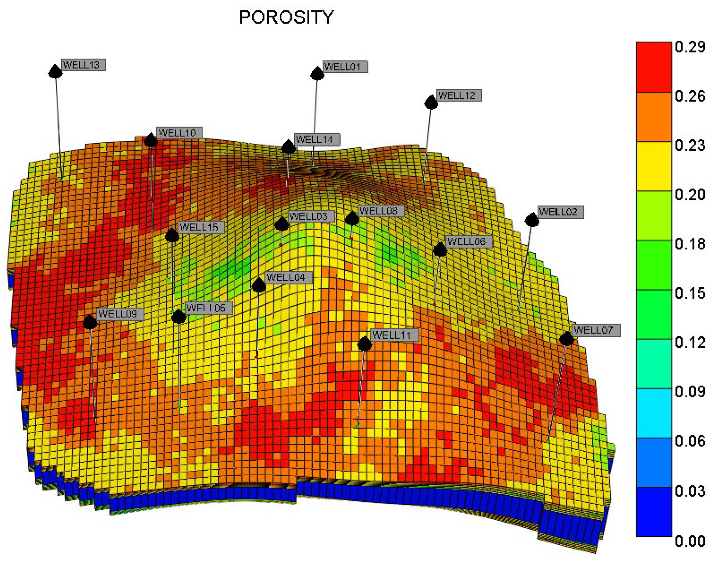
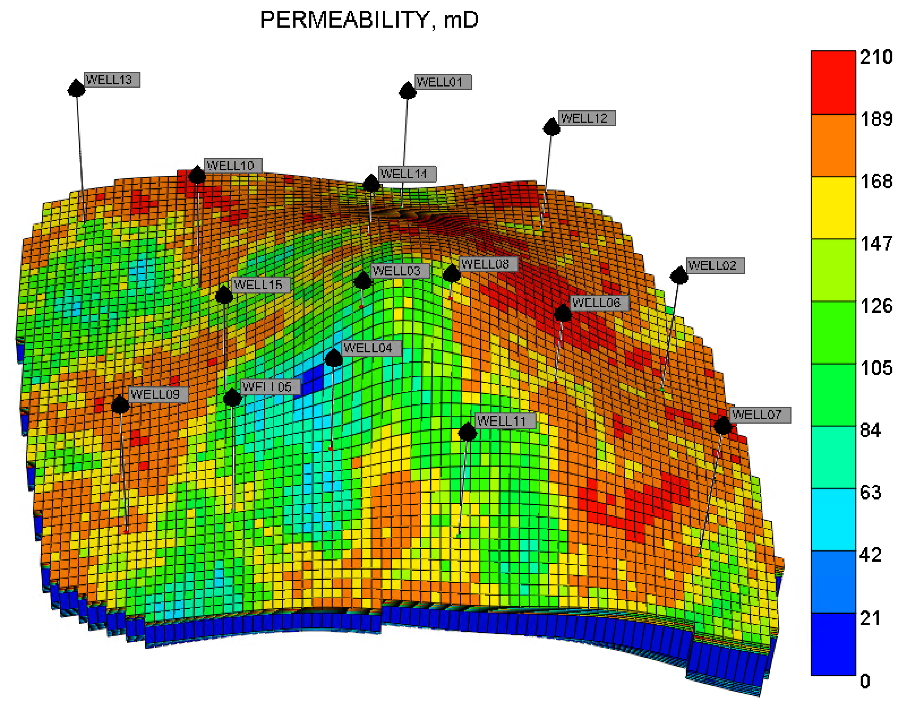
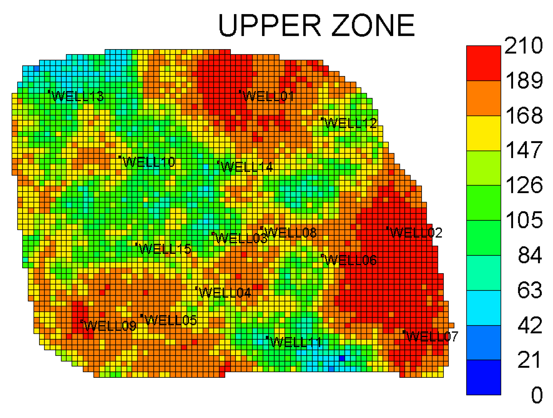
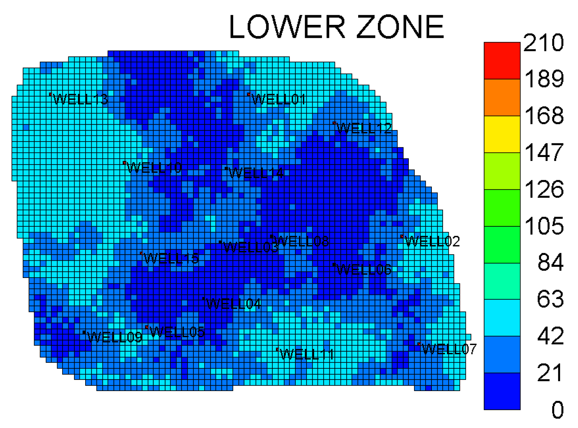
3.1. Reservoir Characterization

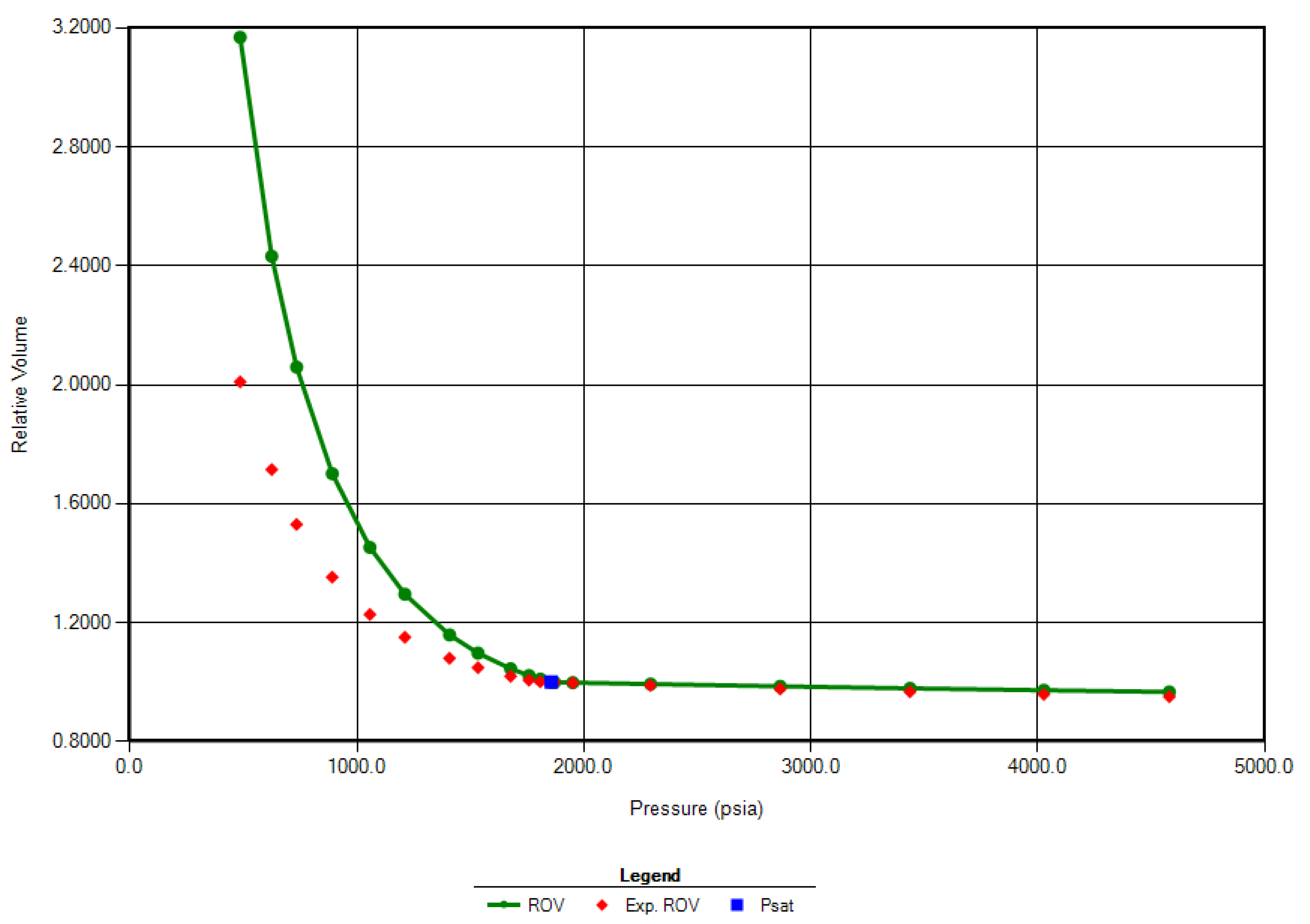
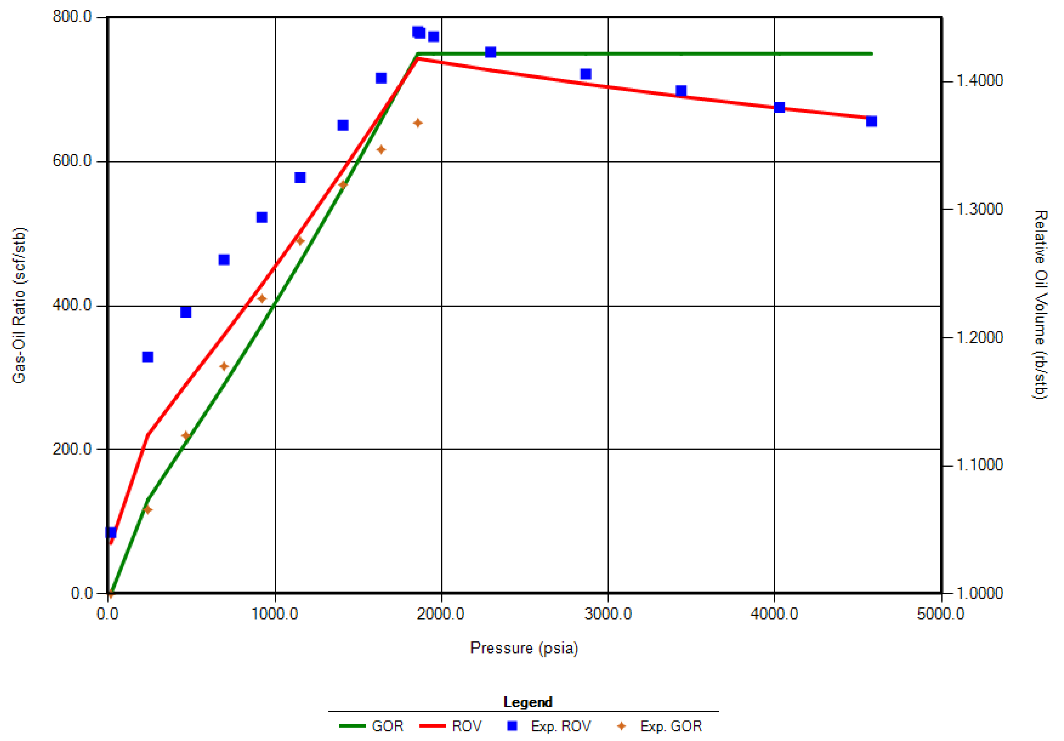
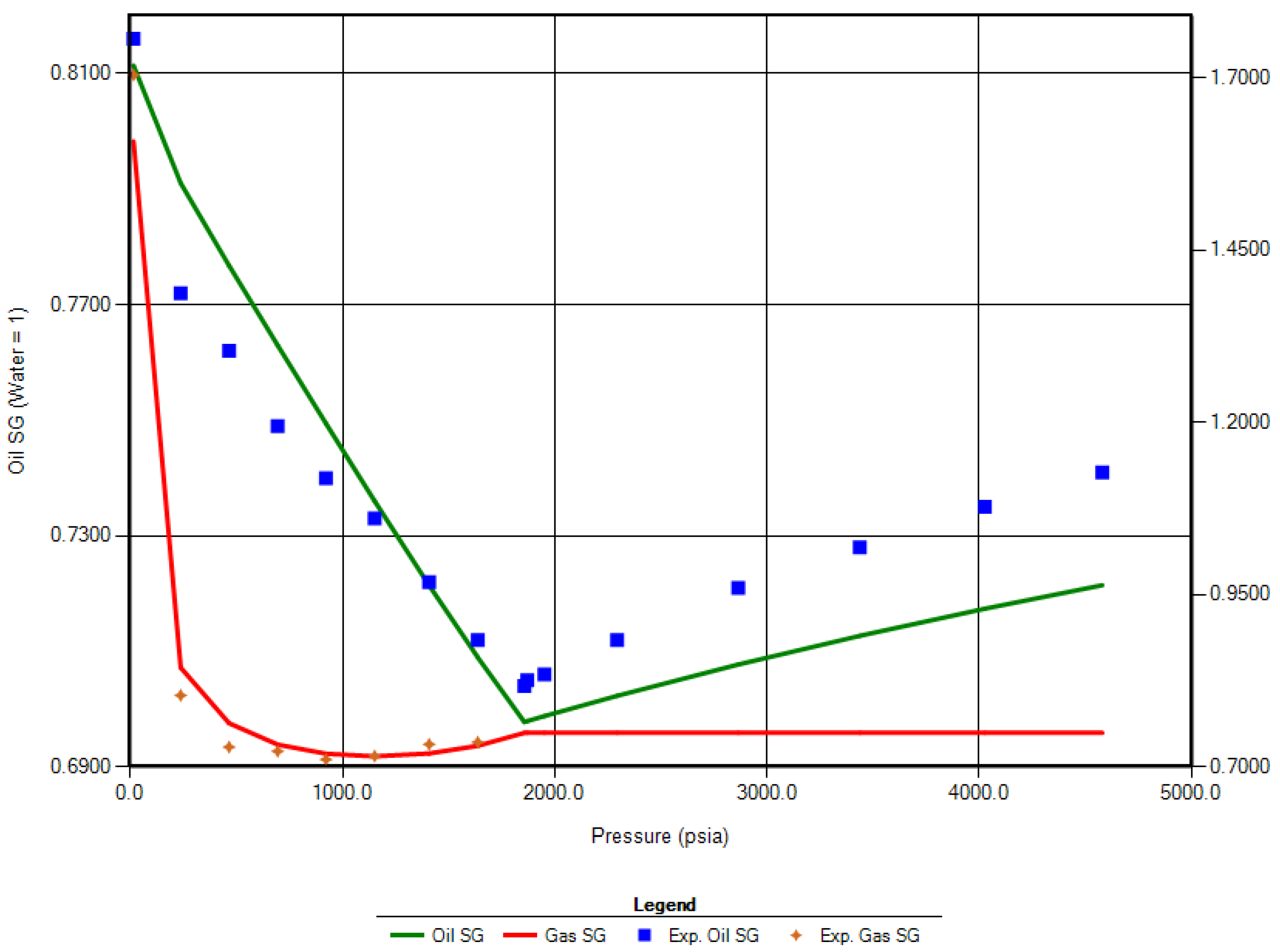
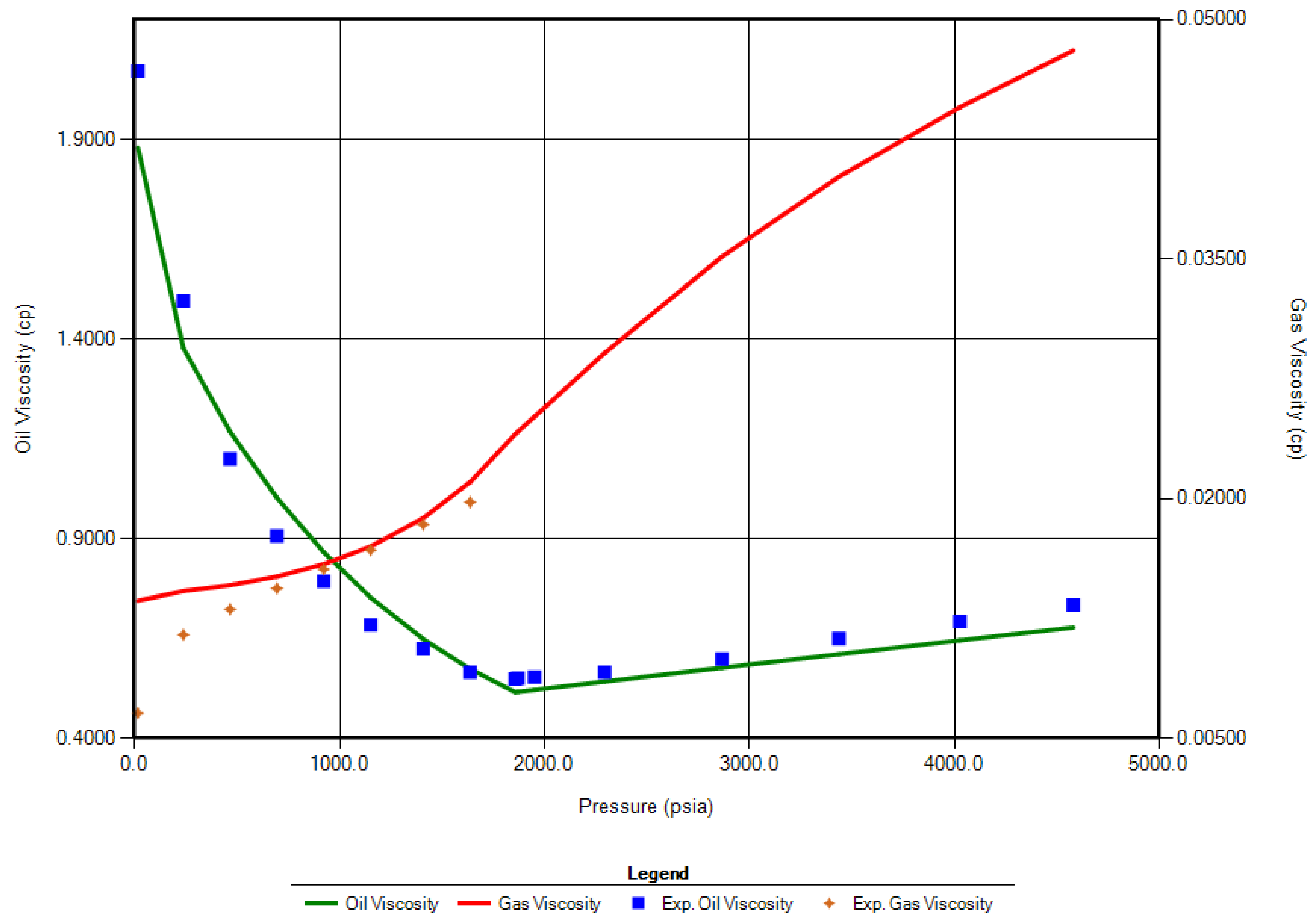
The data used in this study represent an actively producing formation in the Eastern Mediterranean region. The reservoir comprises two distinct productive oil zones separated by an impermeable shale (Figure 5). The density log, and therefore the density porosity, is available for all of the 15 studied wells. Yet only five of them have laboratory measurements of porosity and permeability. Using porosity log data from the 15 wells, the porosity map of upper and lower reservoirs was populated as shown in Figure 5 using Gaussian random function simulation. Looking at the porosity histogram, the upper reservoir is composed of a high-porosity clean sand formation with a more uniform distribution from 20 to 25% and an average of 22%. In contrast, the lower reservoir contains low-porosity tight sand with a wide range spreading from 13% to 29%. A detailed workflow to step-by-step building a static geological model is presented in [20,21]. In addition, structural modeling revealed an anticlinal reservoir structure, which is highly suitable for CO₂-enhanced oil recovery with gravity assistance when CO₂ is injected into the upper portion of the reservoir [22].

Several approaches to correlate permeability with porosity were presented in a previous work [23]. Based on the findings from previous research, a machine learning workflow was implemented to determine the field permeability from well log and core data. The K-means clustering technique was applied to determine the different hydraulic flow units by identifying the optimal cluster number using the elbow method. For each of the obtained clusters, correlations were developed to predict field permeability using gamma ray, bulk density, and porosity data through a regression process, where the linear regression and Support Vector Machine algorithms were found to provide the best accuracy when implemented to characterize the reservoir permeability as compared to the other machine learning algorithms that were utilized. The incorporation of these machine learning-derived permeability estimates into history-matched reservoir models resulted in minimal error when compared to the observed data. Using the presented method, the permeability of the upper and lower reservoir was populated as shown in Figure 6.

As stated above, the reservoir presents two distinct hydraulic flow units, therefore containing two zones with very different permeability distributions. Figure 7 and Figure 8 depict the permeability maps at the middle of the upper and lower reservoir to show more details. The permeability maps indicate a high-heterogeneity sandstone formation, inferring more complicated fluid flow behaviors.

3.2. Fluid Model

In this study, we analyzed a reservoir fluid sample consisting of 30 different hydrocarbon components. Common practice in compositional simulation is to tune the fluid model using the equation of state (EOS) to predict fluid behavior under varying pressure and temperature conditions [24,25]. To successfully match laboratory-measured data with the fluid model predictions, simplifying the fluid composition by combining several components into pseudo-components is often necessary [26]. One proven successful lumping technique suggests combining C1 and N2 as one pseudo-component, C2 to C4 as a second, C5 and C6 as a third, and C7+ divided into three additional pseudo-components based on molecular weights or boiling points [27,28]. In this compositional simulation, seven pseudo-components were lumped, as presented in

Table 4. Mole fraction of pseudo-components.

Component	Mole Fraction
CO2	0.0015
N2 to CH4	0.4206
C2H6_IC4	0.1183
NC4 to FC7	0.1109
FC8_FC12	0.1526
FC13_C19	0.1053
FC20_30+	0.0908
Total	1

.

In EOS modeling, techniques of combining components, matching PVT laboratory data and saturation pressure data using regression, and calculating the multiple miscibility contact were performed. First, a good match between pressure saturation was obtained, where the simulation showed 1856.2 psi in comparison with 1857 psi from the PVT data. The laboratory data from constant composition expansion (CCE) and differential liberation (DL) tests were matched with the tuning fluid model, as shown in Figure 9, Figure 10, Figure 11, and Figure 12. The calculated multiple miscibility contact for the tuned fluid model is 2648 psi. This value will be verified with the result from a 1D slim-tube simulation test in the next section.

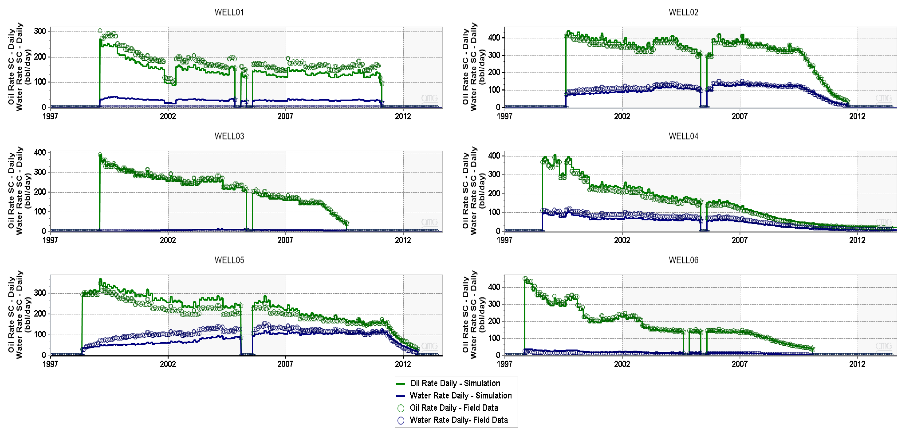
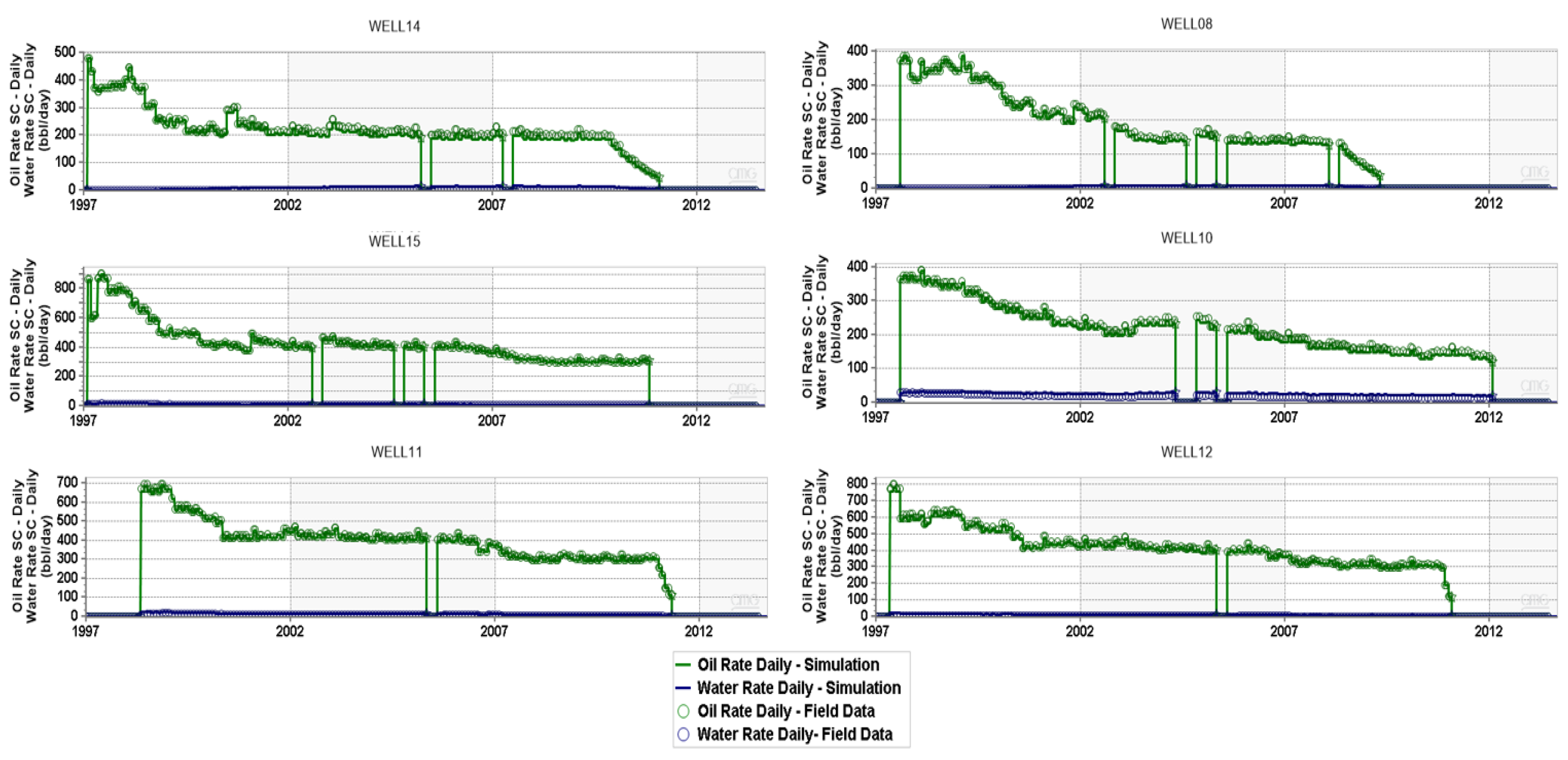
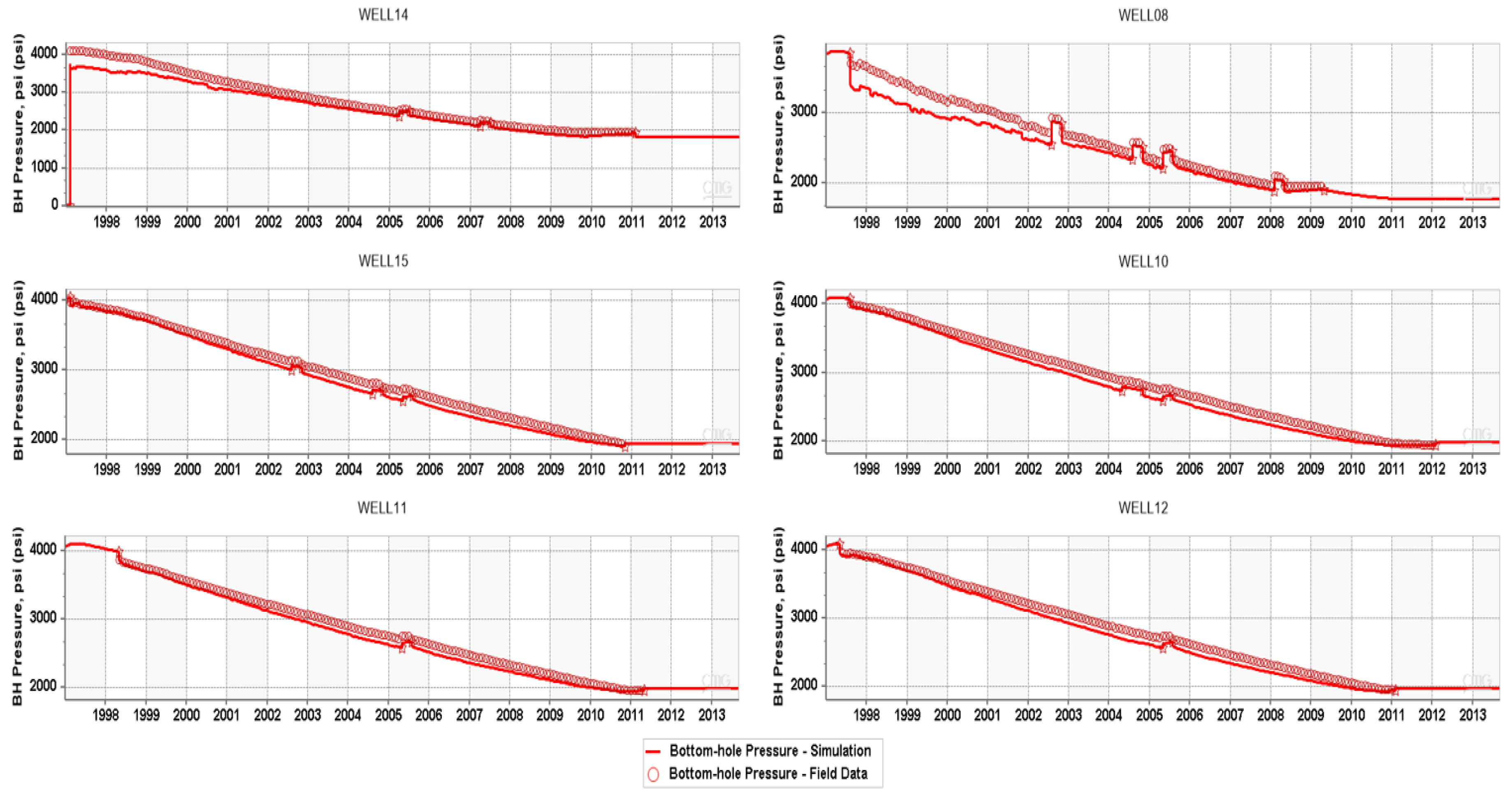
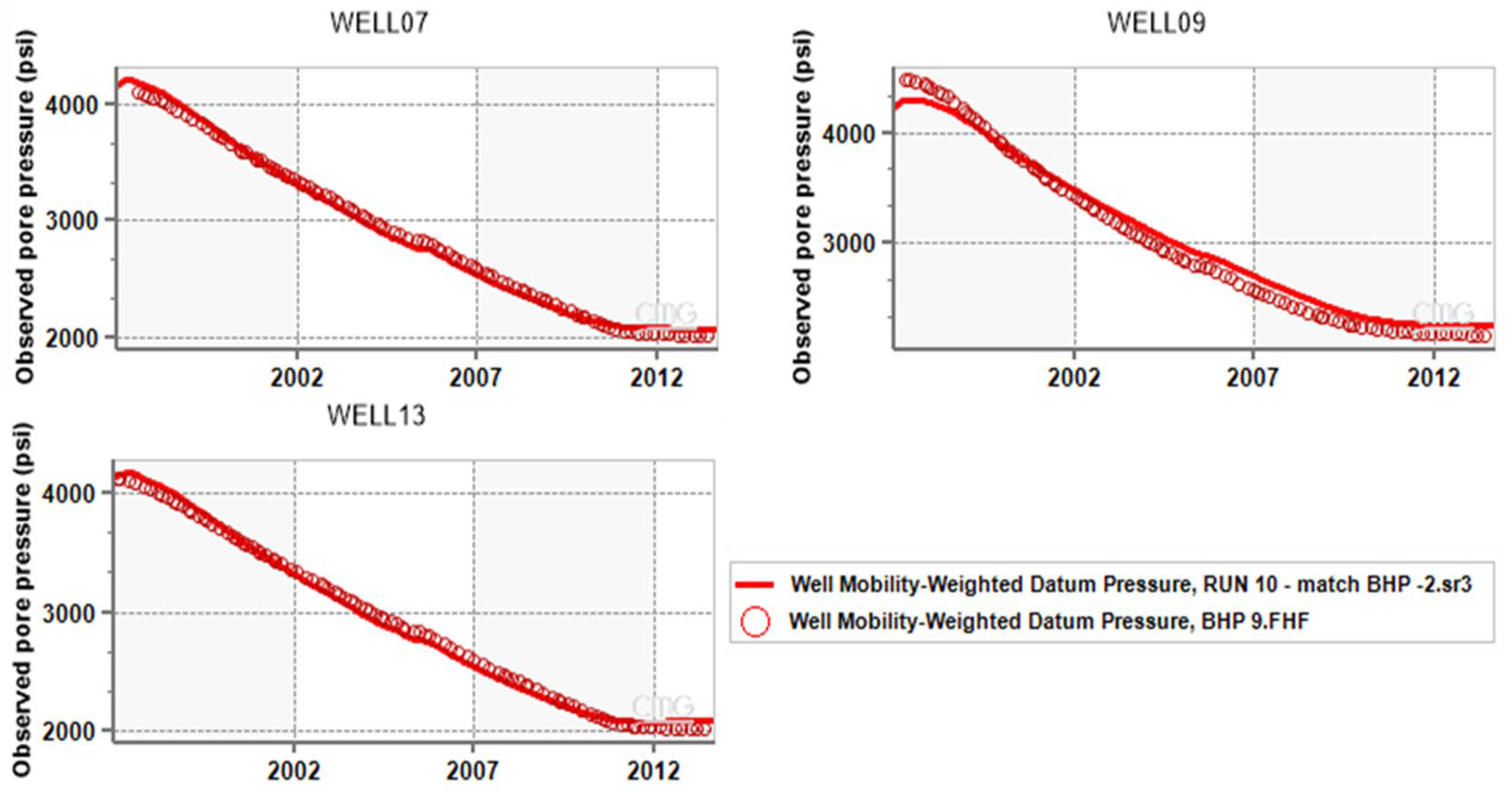
3.3. History Matching

After obtaining the reservoir properties and fluid model, the static model was finalized. Twelve production wells were in operation for 15 years from 1997 to 2013. Traditional history matching techniques were employed to reduce the difference between the simulated and observed values. While history matching has a wide range of applications, such as calibrating subsurface stress changes utilizing geophysical data, this study primarily aims to fine-tune the reservoir hydrodynamic model using field production data. The field history data contain oil and water production, bottom hole pressures, the observed pore pressure for three monitor wells, and the average reservoir pressure. An optimization history matching-assisted workflow by Bui et al. [29] partitioned history matching into two stages. In the first stage, a sensitivity analysis was run to determine the most sensitive parameters affecting oil and water production.

In the second stage, the model can be run through thousands of iterations to obtain the most accurate combination of parameters of reservoir characterizations and completions. The sensitivity analysis showed that the water–oil contact (WOC) of both layers and the partially surrounded aquifers’ properties, including the porosity, permeability, thickness, radius, and initial pressure of the aquifers, are the most sensitive parameters. Using the above understanding of the formation, the history matching process was conducted by locally adjusting uncertain parameters until a good match was achieved. In this study, a thorough history matching process was performed, resulting in a less than 1% deviation of field cumulative production, as shown in Figure 13. Oil and water production rates as well as the bottom hole pressure of individual producers were matched, as depicted in Figure 14, Figure 15, Figure 16, and Figure 17. The matched observed pressure data from the three monitors are illustrated in Figure 18, showing a good match with less than 3% error. The final matching parameters are presented in

Table 5. Summary of history matching parameters.

Component	Mole Fraction
WOC upper reservoir	8410 ft
WOC lower reservoir	8395 ft
Aquifer thickness	20 ft
Aquifer porosity	0.23
Aquifer permeability	27 mD
Radius ratio	2
Initial aquifer pressure	4370 psi

.

3.4. EOR Scenarios

Following the completion of primary production (14 MMSTB), several simulation scenarios are implemented in order to forecast secondary and tertiary production. The production wells’ pressures in reservoir conditions are maintained at 1950 psi. The cumulative oil recoveries, in some cases, are then evaluated in terms of economics to determine the best EOR for actual field adoption.

(a)

15-year water flooding

Secondary production is accomplished through water injection over a 15-year period right after natural reservoir recovery. To optimize the process, a total of six wells (13, 9, 7, 5, 4, and 2) in various locations are assigned for water injection. The reservoir pressures in injection wells are controlled at 4207 psi to obtain the optimal injection rate of water. The 36 MMSTB of oil production is increased further to mark water flooding, achieving total oil recovery of 50 MMSTB.

(b)

15-year continuous CO₂ injection after 15-year water flooding

CO₂ injection is regarded as an effective method for enhancing oil recovery by complying with secondary production through water flooding. Two wells (3 and 8) with different injection strategies for continuous CO₂ injection over 15 years are established to simulate the total oil production:

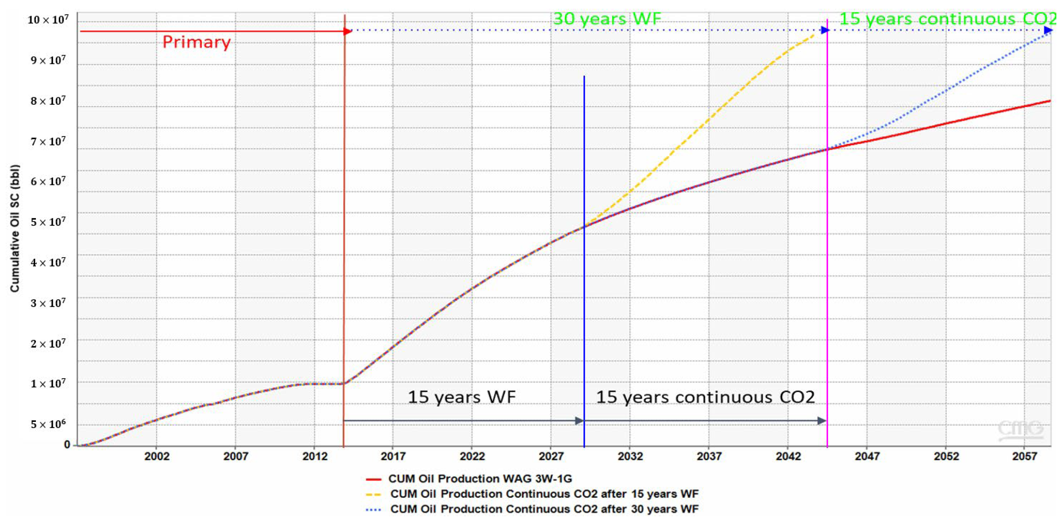
• Firstly, 3.0 MMSCFD is continuously injected through each well over a 15-year period, and the cumulative oil recovery is recorded at 59.7 MMSTB.
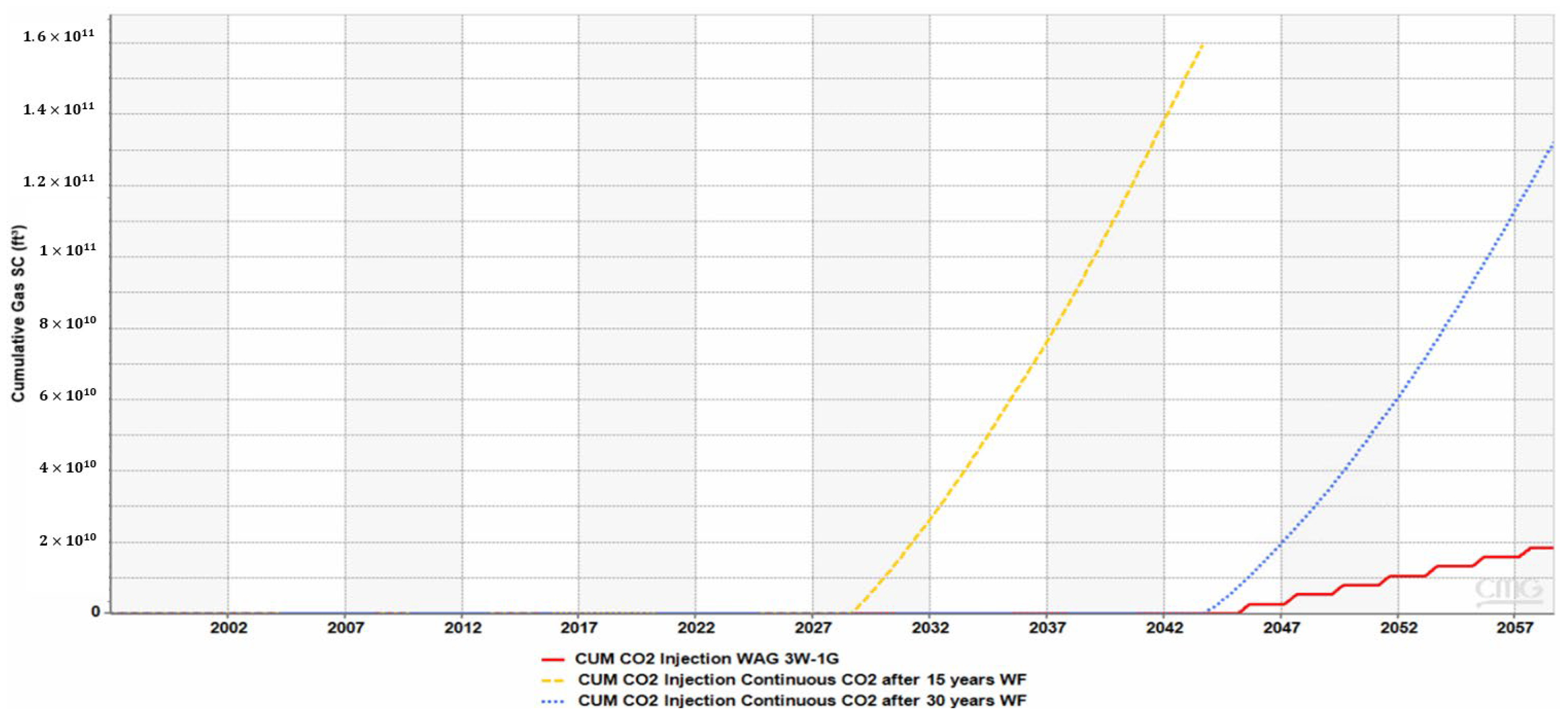
• Secondly, the bottom hole pressures (BHPs) of the injectors are constrained at 2700 psi, which is the minimum pressure to trigger the miscible condition of CO₂ in reservoir fluid, to monitor the maximum required rate of CO₂ injection and oil and water production (Figure 19). The total amount of oil is significantly recovered at 97 MMSTB (Figure 20). The CO₂ volume, on the other hand, is initially injected at 8–10 MMSCFD into each well and peaks at 15–20 MMSCFD at the end of the operation. This continuous CO₂ approach necessitates an aggregate of 8.52 million tons (Mt) (

  Table 6. A summary of the EOR scenarios.

  Case	Scenario	Period (Years)	Well	Cumulative Oil Recovery (MMSTB)/ Recovery Factor %	Remark (Mt: Metric ton)
  1	Water flooding	15	13, 9, 7, 5, 4, 2	50/ 19.6%	4705 psi for injectors and 1950 psi for producers
  2	Continuous CO2 after 15-year WF	15	3, 8	59.7/ 23.4%	CO2 injection rate = 2–3 MMSCFD
  3	Continuous CO2 after 15-year WF	15	3, 8	97/ 38%	Set max BHP = 2700 psi CO2 injection rates: well 3 = 10–20 MMSCFD; well 8 = 8–15 MMSCFD. Total CO2 injected = 8.52 × 106 Mt; total produced = 1.69 × 106 Mt (recycled 20%, total purchased 6.83 × 106 Mt)
  4	Water flooding	30	13, 9, 7, 5, 4, 2	69/ 27%	4705 psi for injectors and 1950 psi for producers
  5	Continuous CO2 after 30-year WF	15	3, 8	76.1/ 29.8%	CO2 injection rate = 2–3 MMSCFD. Total CO2 injected = 1.56 × 106 Mt; total produced = 1.04 × 105 (recycled 7%, total purchased 1.45 × 106 Mt)
  6	Continuous CO2 after 30-year WF	15	3, 8	97.3/ 38.1%	Set max BHP = 2700 psi; CO2 injection rates: well 3 = 7–17.5 MMSCFD Total CO2 injected = 1.03 × 107 Mt; produced = 4.11 × 106 Mt (recycled 40%, total purchased 6.19 × 106 Mt)
  7.1	WAG after 30-year WF (1W:1G Cycle)	15	4, 5, 6, 10	83.4/ 32.6%	BH injection: water = 2000 BBD; CO2 = 11,230 ft3/day (total of 4 wells SC = 14.4 MMSCFD; each well around 3.6 MMSCFD). Total CO2 injected/year = 1.95 × 106 Mt; total produced = 8.58 × 105 Mt (recycled 44%, total purchased 1.09 × 106 Mt)
  7.2	WAG after 30-year WF (2W:1G Cycle)	15	4, 5, 6, 10	83.2/ 32.6%	BH injection: water = 4000 BBD; CO2 = 11,230 ft3/day (total of 4 wells SC = 14.4 MMSCFD; each well around 3.6 MMSCFD). Total CO2 injected/year = 1.31 × 106 Mt; total produced = 5.26 × 105 Mt (recycled 40%, total purchased 7.81 × 105 Mt)
  7.3	WAG after 30-year WF (3W:1G Cycle)	15	4, 5, 6, 10	83.1/ 32.5%	BH injection: water = 6000 BBD; CO2 = 11,230 ft3/day (total of 4 wells SC = 14.4 MMSCFD; each well around 3.6 MMSCFD). Total CO2 injected/year = 8.90 × 105 Mt; total produced = 3.38 × 105 (recycled 38%, total purchased 5.53 × 105 Mt)
  7.4	WAG after 30-year WF (1G:1W Cycle)	15	4, 5, 6, 10	83.3/ 32.6%	BH injection: water = 2000 BBD; CO2 = 11,230 ft3/day (total of 4 wells SC = 14.4 MMSCFD; each well around 3.6 MMSCFD). CO2iInjected = 2.22 × 106 Mt; produced 1.01 × 106 Mt (recycled 45%, total purchased 1.21 × 106 Mt)

  ) to enhance oil recovery by 47 MMSTB. Even though the simulation reveals that 20% of CO₂ can be recycled, the total purchased CO₂ demands 6.83 million Mt.

(c)

30-year water flooding

To assess oil production after the primary process, another water flooding concept is tested over 30 years with settings similar to those of the 15-year case. Six water injectors would sweep the reservoir fluid and contribute an overall oil recovery of 69 MMSTB.

(d)

15-year continuous CO₂ injection after 30-year water flooding

Wells 3 and 8 have been retained under two conditions for continuous CO₂ injection over 15 years after the 30 years of water flooding to visualize the requirements and comparable oil production enhancement:

• The daily injection rate of 3 MMSCF would improve oil mobility in the reservoir and reach the maximum exploitation of 76.1 MMSTB after 15 years. However, this process would only recycle 7% of the pumped CO₂ gas and would require a CO₂ procurement of 1.45 million Mt.
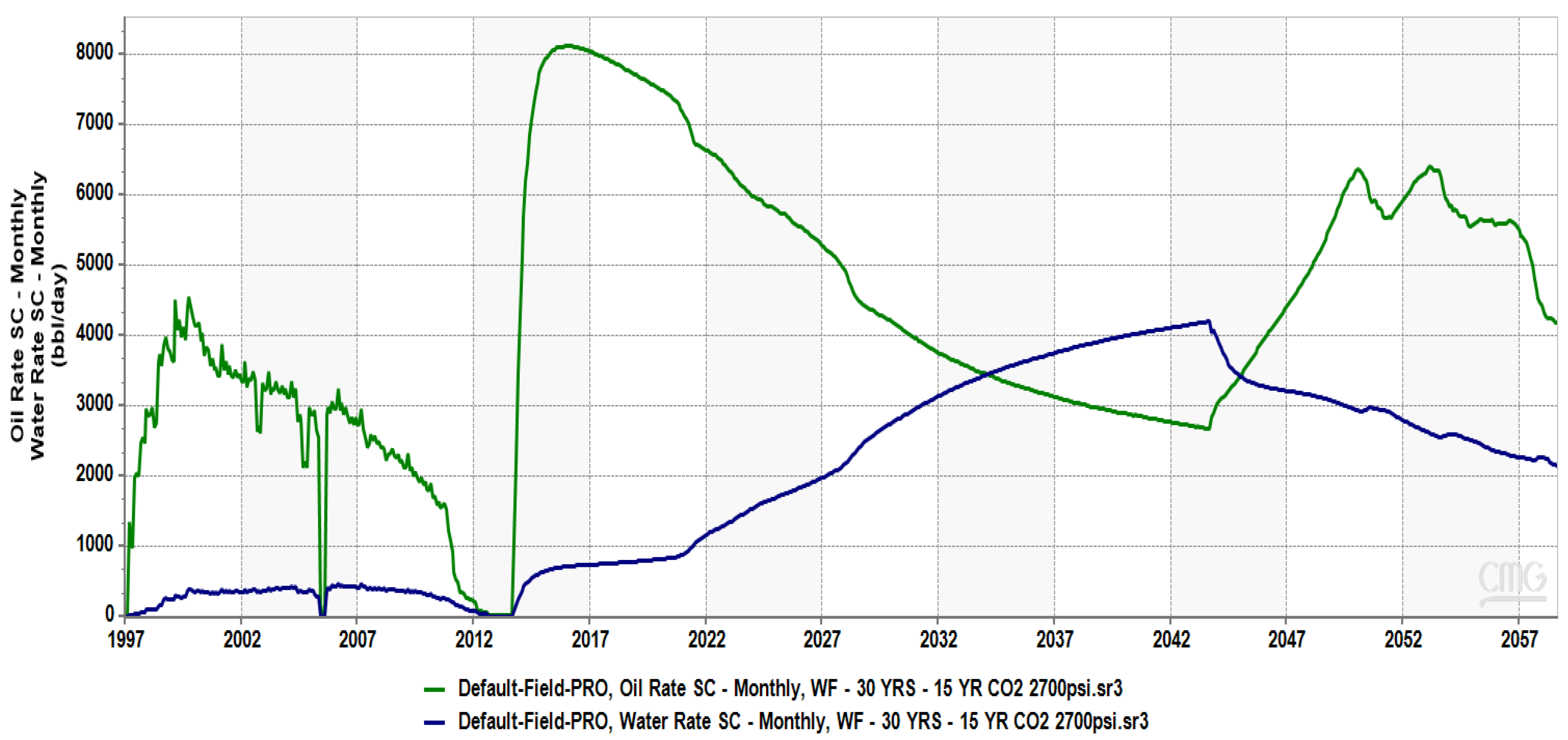
• In contrast, 2700 psi is conditioned as the maximum injection BHP, and the wells must inject gas at a rate ranging from 7 to 17.5 MMSCFD. By injecting a total of 10.3 million Mt CO₂, the simulated result updates the cumulative oil recovery of 97.3 MMSTB (Figure 20), with the oil and water production rates shown in Figure 21. The gas recycling process can achieve 40% efficiency throughout the operation, but the CO₂ purchase mass is estimated to be 6.19 million Mt.

(e)

15-year water-alternating-gas (WAG) injection after 30-year water flooding

The WAG injection, which combines the benefits of both water flooding and CO₂ injection, allows for the alternating injections of CO₂ and water into the reservoirs. The CO₂ dissolves in the crude oil, reducing its viscosity and improving its mobility, while the water creates a pressure front, pushing the oil toward the production well.

From the perspective of simulation, two wells, 5 and 10, are designed to inject the alternating water and CO₂ into the upper production reservoir (after 30-year water flooding, the lower reservoir at wells 5 and 8 is completely saturated by water), while the other two wells, 4 and 6, would operate under the WAG injection in both the upper and lower reservoirs.

In reservoir conditions, the daily injection rates have been configured at 2000 bbls and 11,230 ft3 for water and CO₂, respectively, to keep the injection pressure at 2800 psi (Figure 21), which is higher than the MMP of 2700 psi (Figure 22). Different WAG cycles are set up for the simulation to evaluate the EOR:

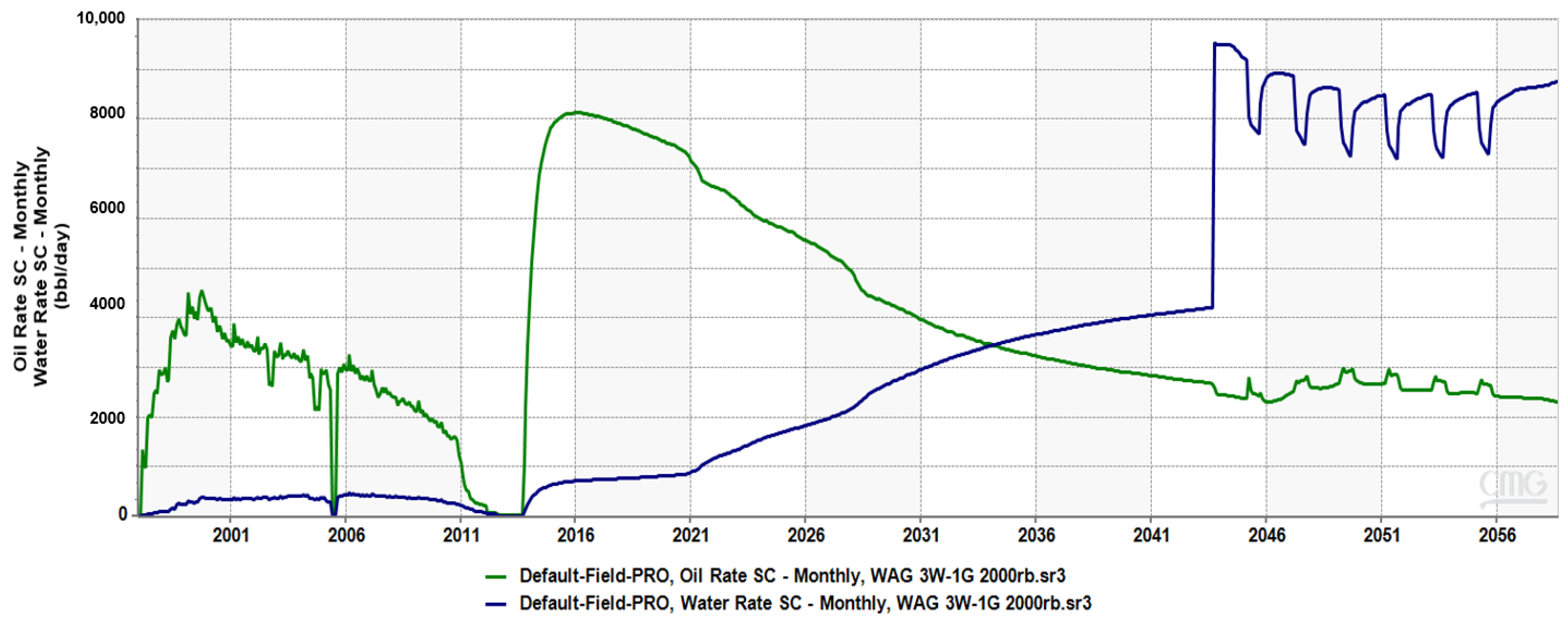
• 1:1 Cycle (water-first chasing): The process is designed to inject water and gas alternately every 12 months. After 15 years, a total mass of 1.95 million Mt CO₂ is injected to accomplish 83.4 MMSTB for cumulative oil recovery. This 1:1 WAG cycle would bring 44% of the injected CO₂ to the surface, requiring the operation to purchase 1.09 million Mt.
• 2:1 Cycle (water-first chasing): The process is tested to alternatively inject water for 16 months and gas for 8 months. Total oil production reaches an amount of 83.2 MMSTB, but the injected volume of CO₂ is equivalent to 1.31 million Mt, which is less than 34% compared to the 1:1 cycle. This scenario involves a CO₂ purchase of 0.78 million Mt.
• 3:1 Cycle (water-first chasing): The final water-first chasing scenario in the WAG test is performed for 18 months for water injection and 6 months for CO₂ injection. The total amount of injected CO₂ in the entire operation is reduced to 0.89 million Mt (Figure 23) (less than 54% of 1:1 cycle and 32% of 2:1 cycle), but the cumulative oil recovery remains at 83.2 MMSTB, with the oil and water production rates displayed in Figure 24. Furthermore, the recycled CO₂ gas in this process is proportional to 38%, requiring a 0.55 million Mt CO₂ purchase.
• 1:1 Cycle (gas-first chasing): The simulation is also activated for gas-first injection to evaluate and compare oil recovery and CO₂ utilization efficiency. The chasing method still involves injecting gas and water alternately every 12 months. The result reveals that total oil production would peak at 83.3 MMSTB if 2.22 million Mt was injected, which is 12% higher compared to the 1:1 cycle of water-first injection.

Figure 20 illustrates the cumulative oil recovery for three EOR schemes: WAG injection, 15 years of continuous CO₂ injection following 15 years of water flooding, and 15 years of continuous CO₂ injection after 30 years of water flooding. Among these, continuous CO₂ injection proves to be the most effective strategy, particularly for the reservoir under consideration. Continuous CO₂ injection achieves its superior performance through several mechanisms. It reduces oil viscosity by dissolving into the oil and achieves near-miscible or fully-miscible conditions under appropriate pressure and temperature. These conditions reduce interfacial tension, swell the oil, and enhance displacement efficiency. The anticlinal of the reservoir further facilitates these processes by providing a gravity-stable environment, which supports miscibility and maintains reservoir pressure near the top of the formation. However, careful flood design is critical to avoid premature CO₂ breakthrough at production wells located at higher elevations in the formation.

The results demonstrate that continuous CO₂ injection outperforms WAG injection due to gravity segregation. During WAG injection, gas tends to rise, and water settles at the bottom, trapping oil in the middle layers and reducing vertical sweep efficiency. This segregation process can cause earlier gas breakthrough and lower overall recovery. The simulation results in Figure 20 highlight the increase in cumulative oil recovery after switching to continuous CO₂ injection. The comparison between CO₂ injection after 15 years and 30 years of water flooding underscores the importance of timing in maximizing recovery.

For the purpose of comparing different scenarios, the CO₂ injection period in all cases is 15 years. The only variations are in the order of water and gas injection or the water flooding duration, which ranges from 15 to 30 years, enabling us to determine the optimal operating conditions for maximizing the efficiency of the EOR process. Table 6 provides a summary of ten EOR scenarios.

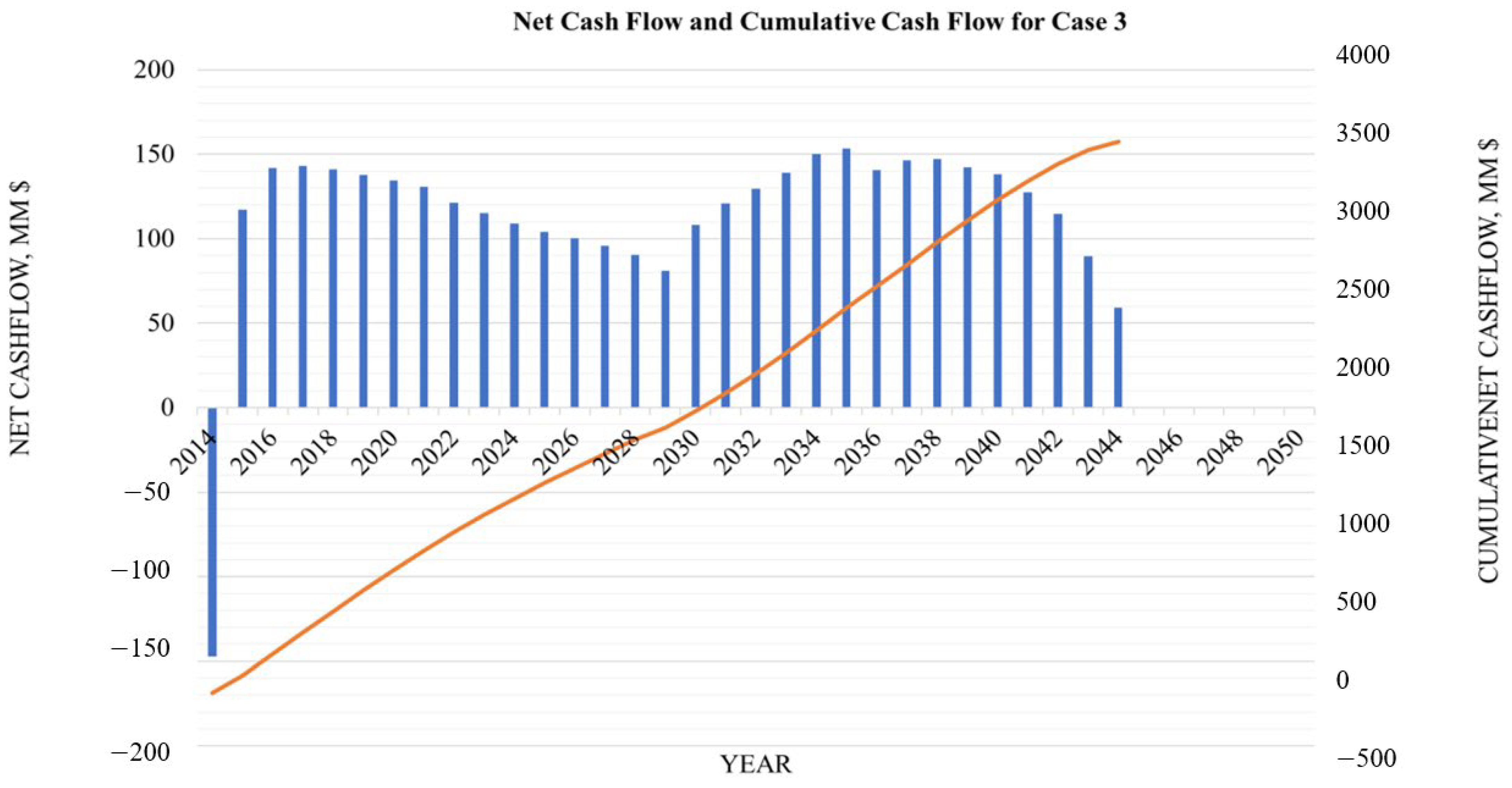
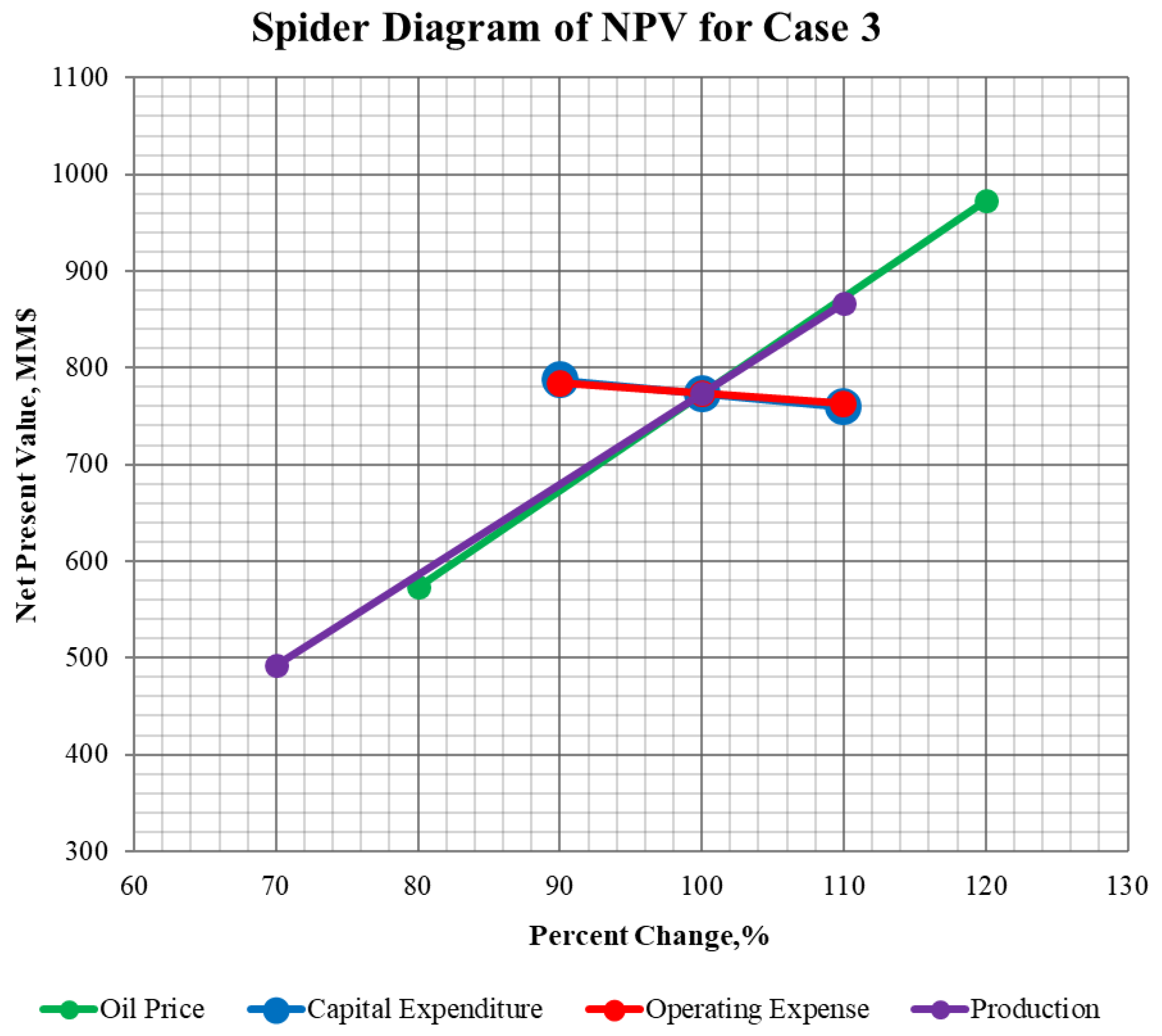
3.5. Economic Analysis

This section presents the results of the economic analysis conducted on the three development scenarios, Case 3, Case 6, and Case 7.3, which outperformed the other cases in the WAG cluster by having the lowest amount of CO₂ injected each year but delivered equivalently cumulative oil recovery. The selection of the three development scenarios was primarily based on cumulative oil production.

Table 7. Capital expenditure comparison of the top three best-case scenarios.

Parameters	Case 3	Case 6	Case 7.3
CO2 recycling plant capital, USD/MM	8.67	15.24	6.64
Compressor cost, USD/MM	78.12	71.62	42.50
Cost of acquiring central batteries (Tanks), USD/MM	0.02	0.02	0.02
Cost of fluid-gathering system, USD/MM	14.60	14.60	14.60
Well injection pumps and wellheads, USD/MM	2.10	2.80	2.80
CO2 distribution line cost, USD/MM	54.20	54.20	36.20
Workovers, USD/MM	0.07	0.07	0.07
Total capex, USD/MM	157.78	158.55	102.84

and

Table 8. Operating expenditure comparison of the top three best-case scenarios.

Parameters	Case 3	Case 6	Case 7.3
Surface Facility Maintenance, USD/MM	330.32	335.12	272.27
Electricity Costs, USD/MM	85.58	70.74	9.79
Water Costs, USD/MM	1.04	11.03	12.90
Water Treatment, USD/MM	4.13	9.88	12.13
CO2 Purchase, USD/MM	252.23	156.35	22.35
CO2 Treatment, USD/MM	22.07	36.48	4.79
Total OPEX, USD/MM	695.38	619.60	334.23

provide detailed insights into the capital expenditures (CAPEXs) and operating expenditures (OPEXs) for Case 3.

Table 7 provides a detailed breakdown of the CAPEX associated with the top three development scenarios: Case 3, Case 6, and Case 7.3. It outlines the costs involved in various key components such as the CO₂ recycling plant capital, compressor costs, and the acquisition of central batteries (tanks). Additionally, the table highlights the investment needed for the fluid-gathering system, well injection pumps and wellheads, CO₂ distribution lines, and workover operations. Each of these components contributes to the total CAPEX required for the development of each case, providing a comprehensive view of the financial outlay needed to execute these scenarios.

Table 8 outlines the OPEX for the three best-case development scenarios. The table captures several key operational cost elements, including the expenses related to surface facility maintenance, electricity consumption, and water use. Additionally, it details the costs involved in water treatment, the purchase of CO₂, and CO₂ treatment processes for each case.

Table 9. Input parameters for OPEX, taxes, royalties, and cost calculations.

Parameters	Value
Surface facility maintenance (fixed daily rate), USD	200,000
Surface facility maintenance, USD/bbl	4
Water cost (contract), USD/bbl of water	0.14
Compression costs, USD/MMcf	188.72
Power costs, USD/HP	2.88
CO2 treatment costs, USD/MMcf	700
Water treatment costs, USD/bbl	0.24
CO2 cost (contract), USD/MMcf	2000
Oil price (@ global market), USD/bbl	75
Interest rate, %	12
Royalty, %	15
State tax, %	3.75
Federal tax, %	18.5

is used to provide the key input parameters for calculating operating expenditures (OPEXs), taxes, royalties, and other associated costs in the economic analysis of the development scenarios.

Based on the data presented in

Table 10. Performance and profitability comparison of the top three scenarios during secondary and tertiary production.

Parameter	Case 3	Case 6	Case 7.3
Cumulative Production, MMSTB	81.08	81.53	65.82
Gross Revenue, USD/MM	6081.00	6114.74	4936.26
Total CAPEX, USD/MM	157.78	158.55	102.84
Total OPEX, USD/MM	695.38	619.60	334.23
Total Expenditure, USD/MM	2556.34	2695.29	1862.79
Net Cash Flow, USD/MM	3524.66	3419.45	3073.47
Net Present Value, USD/MM	773.39	670.15	750.99
IRR	88%	83%	136%

, Case 3 stands out as the most compelling scenario for development, primarily due to its high net present value (NPV) of USD 773.39 million, which reflects the greatest long-term financial return among the three cases. While its capital (CAPEXs) and operating expenditures (OPEXs) are slightly higher than for Case 7.3, Case 3 generates a strong net cash flow of USD 3524.66 million, indicating robust profitability after covering all costs. Additionally, although its internal rate of return (IRR) of 88% is lower than that of Case 7.3, it still demonstrates a very healthy return on investment. The combination of a high NPV, solid cash flow, and a competitive IRR positions Case 3 as the optimal choice, offering the greatest long-term value despite its slightly higher initial expenditure (Figure 25).

Figure 26 and Figure 27 illustrate the sensitivity of both the net present value (NPV) and the internal rate of return (IRR) for Case 3 to changes in key factors such as oil price, capital expenditure (CAPEX), operating expenses (OPEXs), and production rates. The NPV diagram shows that oil price has the greatest impact on project profitability, with the NPV rising significantly as oil prices increase. Production also has a strong influence on the NPV, indicating that higher cumulative oil production contributes to increased financial returns. In contrast, OPEX and CAPEX have the least impact compared to oil price and production, showing that variations in initial capital investment and operating expenditures have minimal influence on the overall project revenue.

For the IRR, oil price similarly demonstrates the highest sensitivity, with increasing prices leading to a considerable increase in the internal rate of return. Production also plays a crucial role in improving the IRR, aligning with the NPV trend. Operating expenses exert a smaller impact on the IRR, while CAPEX has a more pronounced effect on the IRR compared to the NPV. This suggests that while upfront capital costs do not significantly affect the total value of the project, they are more important for ensuring a higher rate of return. Together, these analyses emphasize that oil price stability and production efficiency are critical for maximizing both the NPV and the IRR, while managing CAPEX and OPEX can help optimize project profitability.

4. Conclusions

This study presents a comprehensive compositional simulation study and screening process showing that it is feasible to conduct CO₂-EOR following a secondary recovery method of water flooding. The fluid model was fine-tuned successfully using EOS modeling and deployed for MMP calculation. The compositional reservoir model was history-matched successfully, showing an approximately 1% deviation from field cumulative production. Flowing bottom hole pressure and average reservoir pressure data were honored during the history matching process to guarantee that the development strategies were based on the field conditions.

Using the validated model, ten development strategies with respective water flooding, continuous CO₂, and WAG injection were developed to optimize cumulative oil recovery. While 15-year water flooding increases total oil recovery to 50 MMSTB, the 30-year injection of water can extend oil recovery to 69 MMSTB, corresponding with a 38% recovery factor. On the other hand, continuous CO₂ injection following water flooding leads to an additional 40% increase in oil recovery compared to an increase of 20% in production in the WAG process. This study presented a successful example of continuous CO₂ injection using the gravity-assisted mechanism, showing a total recovery of 50% of the original oil in place. Conducting an economic analysis is crucial for determining the viability of field development strategies, considering factors that may impact the project’s NPV. Economic analysis helps decision-makers select a viable project to invest in. In this study, the capital and operating expenditures associated with each proposed development scenario were evaluated, and the net present value (NPV) was estimated. It was observed from the study that continuous CO₂ injection for 15 years after 15 years of water flooding was the most economical method, with an NPV of USD 1 billion. Furthermore, a sensitivity analysis conducted to investigate the project profitability, indicating that the oil price is a critical component in assessing the viability of a project. The CO₂ purchasing cost had a minimal impact on the project’s NPV.

Based on the reservoir simulation and economic analysis, the deployment of continuous CO₂ injection after 15 years of water flooding is recommended to maximize oil recovery. The economic analysis also suggests a total production period of 30 years (including water flooding and CO₂ injection) rather than extending production time to 45 years since the NPV of the last 15 years does not increase significantly. Following the systematic approach of this study, one can elucidate the optimal field development strategy for their field application and the ideal timeframe of each recovery method before moving forward to the next step.

This study highlights the potential of utilizing CO₂-EOR after water flooding, but it is subject to some limitations. First, the accuracy of the compositional reservoir model strongly depends on the quality and availability of historical field data. Any uncertainties and inaccuracies could affect the precision of the history matching process. The assumptions made during the EOS modeling process may vary as compared to other reservoirs with differing geological or fluid properties. Additionally, the economic analysis is based on certain assumptions regarding oil price, the cost of CO₂, the cost of water treatment, and other surface equipment costs. This could affect the viability of the proposed strategies under different market conditions.

In future research, the scope of the sensitivity analysis should be expanded to consider a wider range of economic factors that could impact the project’s NPV. Further exploration of hybrid EOR techniques, such as combining CO₂ injection with chemical or microbial methods, may result in additional increased oil recovery. In the long term, future studies could also investigate the feasibility of carbon sequestration in depleted oil reservoirs when storing CO₂ is considered the most priority.

References

1. Energy, Office of Fossil Energy and Carbon Management; The U.S. Department of Energy. Enhanced Oil Recovery; Energy, Office of Fossil Energy and Carbon Management, The U.S. Department of Energy: Washington, DC, USA, 2023. [Google Scholar]
2. Alfarge, D.; Wei, M.; Bai, B. Fundamentals of Enhanced Oil Recovery Methods for Unconventional Oil Reservoirs; Elsevier: Amsterdam, The Netherlands, 2020. [Google Scholar]
3. Ren, B.; Duncan, I.J. Maximizing oil production from water alternating gas (CO2) injection into residual oil zones: The impact of oil saturation and heterogeneity. Energy 2021, 222, 119915. [Google Scholar] [CrossRef]
4. Alvarado, V.; Manrique, E. Enhanced oil recovery: An update review. Energies 2010, 3, 1529–1575. [Google Scholar] [CrossRef]
5. Bagrezaie, M.A.; Dabir, B.; Rashidi, F.; Moazzeni, A.R. Modeling of formation damage during smart water flooding in sandstone reservoirs. Sci. Rep. 2023, 13, 17564. [Google Scholar] [CrossRef] [PubMed]
6. Jarrell, P.M.; Fox, C.E.; Stein, M.H.; Webb, S.L. Practical Aspects of CO2 Flooding; Society of Petroleum Engineers: Richardson, TX, USA, 2002. [Google Scholar]
7. Verma, M.K. Fundamentals of Carbon Dioxide-Enhanced Oil Recovery (CO2-EOR): A Supporting Document of the Assessment Methodology for Hydrocarbon Recovery Using CO2-EOR Associated with Carbon Sequestration; US Geological Survey: Reston, VA, USA, 2015. [Google Scholar]
8. Afzali, S.; Rezaei, N.; Zendehboudi, S. A comprehensive review on enhanced oil recovery by water alternating gas (WAG) injection. Fuel 2018, 227, 218–246. [Google Scholar] [CrossRef]
9. Elsharafi, M. Literature review of water alternation gas injection. J. Earth Energy Eng. 2018, 7, 33–45. [Google Scholar]
10. Abdullah, N.; Hasan, N. The implementation of Water Alternating (WAG) injection to obtain optimum recovery in Cornea Field, Australia. J. Pet. Explor. Prod. 2021, 11, 1475–1485. [Google Scholar] [CrossRef]
11. Sadeghnejad, S.; Manteghian, M.; Ruzsaz, H. Simulation optimization of water-alternating-gas process under operational constraints: A case study in the Persian Gulf. Sci. Iran. 2019, 26, 3431–3446. [Google Scholar] [CrossRef]
12. Touray, S. Effect of Water Alternating Gas Injection on ultimate Oil Recovery. Master’s Thesis, Engineering Dalhousie University, Halifax, NS, Canada, 2023. [Google Scholar]
13. Rahimi, V.; Bidarigh, M.; Bahrami, P. Experimental study and performance investigation of miscible water-alternating-CO2 flooding for enhancing oil recovery in the Sarvak formation. Oil Gas Sci. Technol. Rev. D’ifp Energ. Nouv. 2017, 72, 35. [Google Scholar] [CrossRef]
14. Zhou, D.; Yan, M.; Calvin, W.M. Optimization of a mature CO2 flood—From continuous injection to WAG. In Proceedings of the SPE Improved Oil Recovery Symposium, Tulsa, OK, USA, 14–18 April 2012. [Google Scholar]
15. AlSeiari, R.A.M.; Bhushan, Y.; Igogo, A.; Singh, M.K.; Al Marzooqi, S.; Al Hammadi, S.A.; Khan, S.H.; Mohamed, M.A.; Brodie, J.; Al Tenaji, A.; et al. A success story of the first miscible CO2 WAG miscible WAG pilots in a giant carbonate reservoir in Abu Dhabi. In Proceedings of the ADIPEC, Abu Dhabi, United Arab Emirates, 31 October–3 November 2022. [Google Scholar]
16. National Energy Technology Laboratory Carbon Dioxide Enhanced Oil Recovery; U.S. Department of Energy: Washington, DC, USA, 2010.
17. McCoy, S.T. The Economics of CO2 Transport by Pipeline and Storage in Saline Aquifers and Oil Reservoirs; Department of Engineering and Public Policy: Pittsburgh, PA, USA, 2008. [Google Scholar]
18. Kwak, D.H.; Kim, J.K. Techno-economic evaluation of CO2 enhanced oil recovery (EOR) with the optimization of CO2 supply. Int. J. Greenh. Gas Control 2017, 58, 169–184. [Google Scholar] [CrossRef]
19. Heddle, G.; Herzog, H.; Klett, M. The Economics of CO2 Storage; Massachusetts Institute of Technology, Laboratory for Energy and the Environment: Cambridge, MA, USA, 2003. [Google Scholar]
20. Ross-Coss, D.; Ampomah, W.; Cather, M.; Balch, R.S.; Mozley, P.; Rasmussen, L. An improved approach for sandstone reservoir characterization. In Proceedings of the SPE Western Regional Meeting, Anchorage, AK, USA, 23–26 May 2016. [Google Scholar]
21. Koray, A.M.; Bui, D.; Kubi, E.A.; Ampomah, W.; Amosu, A. Machine Learning Based Reservoir Characterization and Numerical Modeling from Integrated Well Log and Core Data. Geoenergy Sci. Eng. 2024, 243, 213296. [Google Scholar] [CrossRef]
22. Lu, H.; Xin, X.; Ye, J.; Yu, G. Analysis of factors impacting CO2 assisted gravity drainage in oil reservoirs with bottom water. Processes 2023, 11, 3290. [Google Scholar] [CrossRef]
23. Koray, A.M.; Bui, D.; Ampomah, W.; Appiah Kubi, E.; Klumpenhower, J. Application of machine learning optimization workflow to improve oil recovery. In Proceedings of the SPE Oklahoma City Oil and Gas Symposium/Production and Operations Symposium, Oklahoma City, OK, USA, 17–19 April 2023. [Google Scholar]
24. Gunda, D.; Ampomah, W.; Grigg, R.; Balch, R. Reservoir Fluid Characterization for Miscible Enhanced Oil Recovery. In Proceedings of the Carbon Management Technology Conference, Sugar Land, TX, USA, 17–19 November 2015. [Google Scholar]
25. McCain, W., Jr. The Properties of Petroleum Fluids, 2nd ed.; PennWell Books: Tulsa, OK, USA, 1990. [Google Scholar]
26. Whitson, C.H.; Brulé, M.R. Phase Behavior; Society of Petroleum Engineers: Richardson, TX, USA, 2000. [Google Scholar]
27. Danesh, A. PVT and Phase Behaviour of Petroleum Reservoir Fluids; Elsevier: Amsterdam, The Netherlands, 1998. [Google Scholar]
28. Whitson, C.H.; Sunjerga, S. PVT in Liquid-Rich Shale Reservoirs. In Proceedings of the SPE Annual Technical Conference and Exhibition, San Antonio, TX, USA, 8–10 October 2012. [Google Scholar]
29. Bui, D.; Nguyen, T.; Yoo, H. A Coupled Geomechanics-Reservoir Simulation Workflow to Estimate the Optimal Well-Spacing in the Wolfcamp Formation in Lea County. In Proceedings of the AADE National Technical Conference and Exhibition, Midland, TX, USA, 4–5 April 2023. [Google Scholar]
Figure 1. The impact of gravity during water flooding.
Gases 05 00001 g001
Figure 2. The gravity effect of CO2 injection.
Gases 05 00001 g002
Figure 3. Mechanism of WAG CO2 injection.
Gases 05 00001 g003
Figure 4. Methodology flowchart mapping data collection to development strategies.
Gases 05 00001 g004
Figure 5. Porosity map of studied reservoir.
Gases 05 00001 g005
Figure 6. Calculated permeability of reservoir.
Gases 05 00001 g006
Figure 7. Permeability distribution of upper reservoir.
Gases 05 00001 g007
Figure 8. Permeability distribution of lower reservoir.
Gases 05 00001 g008
Figure 9. The simulated and observed data vs. pressure for the CCE experiment.
Gases 05 00001 g009
Figure 10. The simulated and observed data vs. pressure for the gas–oil ratio and the relative oil volume.
Gases 05 00001 g010
Figure 11. The simulated and observed data vs. pressure for the oil and gas specific gravity.
Gases 05 00001 g011
Figure 12. The simulated and observed data vs. pressure for the oil and gas viscosity.
Gases 05 00001 g012
Figure 13. Field production history matching.
Gases 05 00001 g013
Figure 14. Production history matching of 6 wells.
Gases 05 00001 g014
Figure 15. Production history matching of the other 6 wells.
Gases 05 00001 g015
Figure 16. History matching of bottom hole pressure of 6 production wells.
Gases 05 00001 g016
Figure 17. History matching of bottom hole pressure of the other 6 production wells.
Gases 05 00001 g017
Figure 18. History matching of observed pore pressure of monitoring well.
Gases 05 00001 g018
Figure 19. Oil and water production rates of continuous CO2 injection over 15 years with 2700 psi BHP pressure after 15-year water flooding.
Gases 05 00001 g019
Figure 20. Cumulative oil recoveries in 3 main EOR scenarios.
Gases 05 00001 g020
Figure 21. Oil and water production rates of continuous CO2 injection over 15 years with 2700 psi BHP pressure after 30-year water flooding.
Gases 05 00001 g021
Figure 22. Average reservoir pressures in 3 main EOR scenarios.
Gases 05 00001 g022
Figure 23. Cumulative CO2 injection in 3 main EOR scenarios.
Gases 05 00001 g023
Figure 24. Oil and water production rates of WAG injection over 15 years after 30-year water flooding.
Gases 05 00001 g024
Figure 25. Cumulative and net cash flow of Case 3 during secondary and tertiary recovery.
Gases 05 00001 g025
Figure 26. Sensitivity analysis of NPV for Case 3.
Gases 05 00001 g026
Figure 27. Sensitivity analysis of IRR for Case 3.
Gases 05 00001 g027