
Measurement Uncertainty in the Totalisation of Quantity and Energy Measurement in Gas Grids


Abstract
1. Introduction
2. Volume, Mass, and Energy Measurement
2.1. Framework
2.2. Mass
2.3. Volume
2.4. Energy
- —
- the multiplication of the calculated volume under reference conditions with the averaged calculated calorific value of the same hour;
- —
- in situ energy calculation in the volume conversion device using the actual measured entities for the calculation of energy based on the calculation of and , followed by summing these single energy quantities over 1 .
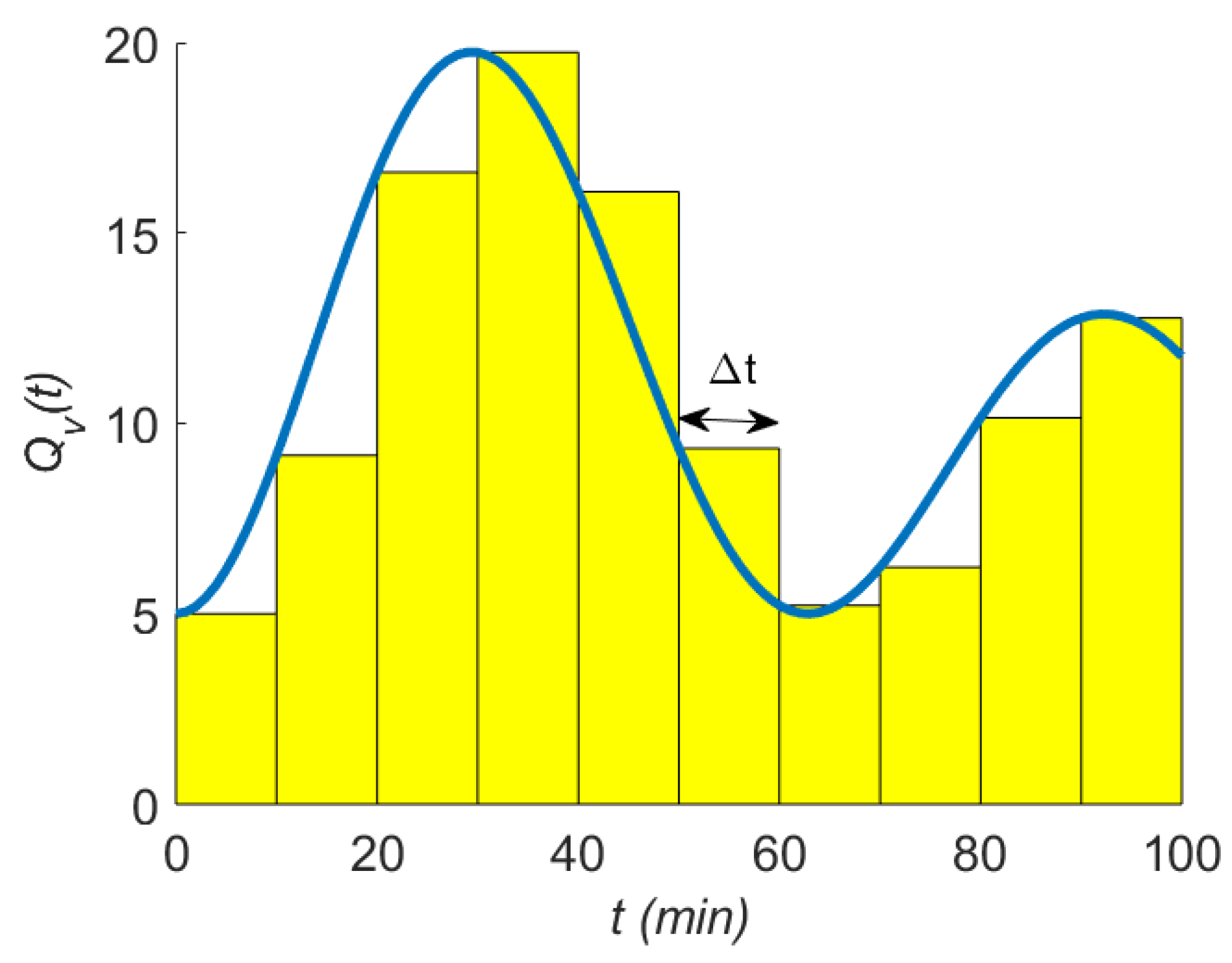
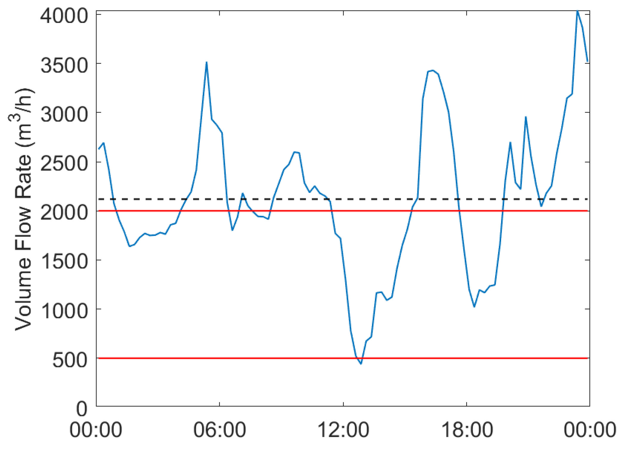
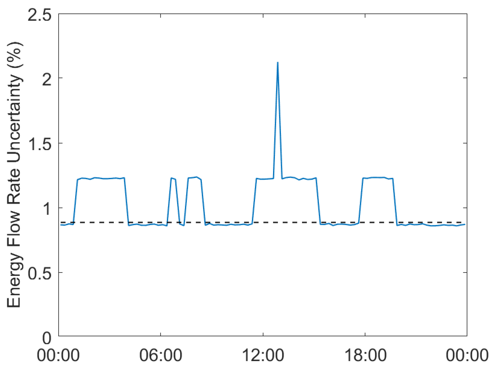
3. Temporal Effects
4. Totalisation
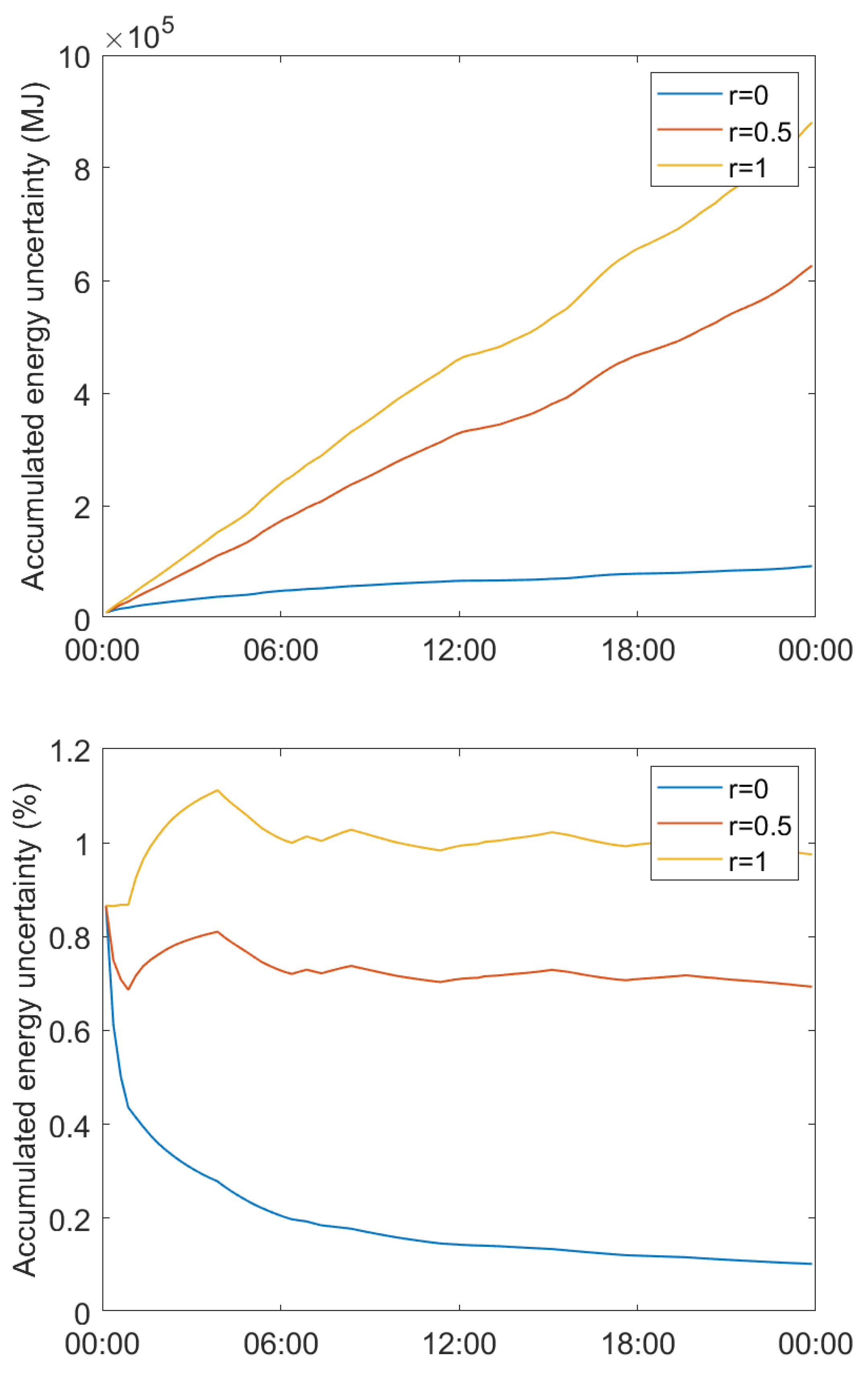
5. Impact of Correlations
6. Discussion and Outlook
Author Contributions
Funding
Data Availability Statement
Conflicts of Interest
Abbreviations
| GC | gas chromatograph |
| GUM | Guide to the Expression of Uncertainty in Measurement |
| ISO | International Organisation for Standardisation |
| JCGM | Joint Committee for Guides in Metrology |
| LPU | law of propagation of uncertainty |
| MCM | Monte Carlo method |
| MDPI | Multidisciplinary Digital Publishing Institute |
| probability density function |
References
- Baker, R.C. Flow Measurement Handbook, Digitally Printed First Paperback Version ed.; Includes Bibliographical References; Cambridge University Press: Cambridge, UK, 2005. [Google Scholar]
- Mokhatab, S.; Poe, W.A.; Speight, J.G. Handbook of Natural Gas Transmission and Processing; Gulf Professional Publishing: Houston, TX, USA, 2006. [Google Scholar]
- Hall, K.; Holste, J. Determination of natural gas custody transfer properties. Flow Meas. Instrum. 1990, 1, 127–132. [Google Scholar] [CrossRef]
- Ficco, G.; Canale, L.; Cortellessa, G.; Zuena, F.; Dell’Isola, M. Effect of flow-rate measurement accuracy on unaccounted for gas in transmission networks. Flow Meas. Instrum. 2023, 90, 102336. [Google Scholar] [CrossRef]
- Ficco, G.; Dell’Isola, M.; Vigo, P.; Celenza, L. Uncertainty analysis of energy measurements in natural gas transmission networks. Flow Meas. Instrum. 2015, 42, 58–68. [Google Scholar] [CrossRef]
- ISO 15112; Natural Gas—Energy Determination. 2nd ed. ISO, International Organization for Standardization: Geneva, Switzerland, 2011.
- EN 1776; Gas Infrastructure—Gas Measuring Systems—Functional Requirements. 2nd ed. CEN, European Committee for Standardization: Brussels, Belgium, 2015.
- OIML R 140; Measuring Systems for Gaseous Fuel. OIML, International Organization for Legal Metrology: Paris, France, 2007.
- ISO 5167-1; Measurement of Fluid Flow by Means of Pressure Differential Devices Inserted in Circular Cross-Section Conduits Running Full—Part 1: General Principles and Requirements. 3rd ed. ISO, International Organization for Standardization: Geneva, Switzerland, 2022.
- ISO 5167-2; Measurement of Fluid Flow by Means of Pressure Differential Devices Inserted in Circular Cross-Section Conduits Running Full—Part 2: Orifice Plates. 3rd ed. ISO, International Organization for Standardization: Geneva, Switzerland, 2022.
- ISO 5167-3; Measurement of Fluid Flow by Means of Pressure Differential Devices Inserted in Circular Cross-Section Conduits Running Full—Part 3: Nozzles and Venturi Nozzles. 3rd ed. ISO, International Organization for Standardization: Geneva, Switzerland, 2022.
- ISO 5167-4; Measurement of Fluid Flow by Means of Pressure Differential Devices Inserted in Circular Cross-Section Conduits Running Full—Part 4: Venturi Tubes. 2nd ed. ISO, International Organization for Standardization: Geneva, Switzerland, 2022.
- ISO 9300; Measurement of Gas Flow by Means of Critical Flow Venturi Nozzles. 3rd ed. ISO, International Organization for Standardization: Geneva, Switzerland, 2020.
- ISO 6974-1; Natural Gas—Determination of Composition with Defined Uncertainty by Gas Chromatography—Part 1: Guidelines for Tailored Analysis. 2nd ed. ISO, International Organization for Standardization: Geneva, Switzerland, 2012.
- ISO 6974-2; Natural Gas—Determination of Composition with Defined Uncertainty by Gas Chromatography—Part 2: Measuring-System Characteristics and Statistics for Processing of Data. 2nd ed. ISO, International Organization for Standardization: Geneva, Switzerland, 2012.
- ISO 6974-3; Natural Gas—Determination of Composition with Defined Uncertainty by Gas Chromatography—Part 3: Determination of Hydrogen, Helium, Oxygen, Nitrogen, Carbon Dioxide and Hydrocarbons up to C8 Using Two Packed Columns. 1st ed. ISO, International Organization for Standardization: Geneva, Switzerland, 2000.
- ISO 6974-4; Natural Gas—Determination of Composition with Defined Uncertainty by Gas Chromatography—Part 4: Determination of Nitrogen, Carbon Dioxide and C1 to C5 and C6+ Hydrocarbons for a Laboratory and On-Line Measuring System Using Two Columns. ISO, International Organization for Standardization: Geneva, Switzerland, 2000.
- ISO 6974-5; Natural Gas—Determination of Composition with Defined Uncertainty by Gas Chromatography—Part 5: Isothermal Method for Nitrogen, Carbon Dioxide, C1 to C5 Hydrocarbons and C6+ Hydrocarbons. ISO, International Organization for Standardization: Geneva, Switzerland, 2015.
- ISO 6974-6; Natural Gas—Determination of Composition with Defined Uncertainty by Gas Chromatography—Part 6: Determination of Hydrogen, Helium, Oxygen, Nitrogen, Carbon Dioxide and C1 to C8 Hydrocarbons Using Three Capillary Columns. ISO, International Organization for Standardization: Geneva, Switzerland, 2002.
- ISO 15970; Natural Gas—Measurement of Properties—Volumetric Properties: Density, Pressure, Temperature and Compression Factor. 1st ed. ISO, International Organization for Standardization: Geneva, Switzerland, 2008.
- ISO 15971; Natural Gas—Measurement of Properties—Calorific Value and Wobbe Index. 1st ed. ISO, International Organization for Standardization: Geneva, Switzerland, 2008.
- JCGM 100:2008; Evaluation of Measurement Data—Guide to the Expression of Uncertainty in Measurement. GUM:1995 with minor corrections. BIPM: Sèvres, France, 2008.
- JCGM 102:2011; Evaluation of Measurement Data—Guide to the Expression of Uncertainty in Measurement—Supplement 2 to the “Guide to the Expression of Uncertainty in Measurement”—Extension to Any Number of Output Quantities. BIPM: Sèvres, France, 2011.
- ISO/IEC 17000; Conformity Assessment—Vocabulary and General Principles. 2nd ed. ISO/IEC, International Organization for Standardization: Geneva, Switzerland, 2020.
- JCGM 106:2012; Evaluation of Measurement Data—The Role of Measurement Uncertainty in Conformity Assessment. BIPM: Sèvres, France, 2012.
- JCGM 101:2008; Evaluation of Measurement Data—Guide to the Expression of Uncertainty in Measurement—Supplement 1 to the “Guide to the Expression of Uncertainty in Measurement”—Propagation of Distributions Using a Monte Carlo Method. BIPM: Sèvres, France, 2008.
- ISO 6976; Natural Gas—Calculation of Calorific Values, Density, Relative Density and Wobbe Indices from Composition. ISO, International Organization for Standardization: Geneva, Switzerland, 2016.
- van der Veen, A.M.H. Credible Uncertainties for Natural Gas Properties Calculated from Normalised Natural Gas Composition Data. Methane 2025, 4, 1. [Google Scholar] [CrossRef]
- van der Veen, A.M.H. Metrology for the Hydrogen Supply Chain; Publishable Summary; EURAMET: Teddington, UK, 2023; Available online: https://www.euramet.org/download?tx_eurametfiles_download%5Baction%5D=download&tx_eurametfiles_download%5Bcontroller%5D=File&tx_eurametfiles_download%5Bfiles%5D=47048&tx_eurametfiles_download%5Bidentifier%5D=%252Fdocs%252FEMRP%252FJRP%252FJRP_Summaries_2021%252FGreen_Deal%252F21GRD05_Publishable_Summary.pdf&cHash=5af7f1295b8a1a749769e2338864ce64 (accessed on 8 August 2024).
- Cox, M.G.; van der Veen, A.M.H. (Eds.) Understanding and treating correlated quantities in measurement uncertainty evaluation. In Good Practice in Evaluating Measurement Uncertainty—Compendium of Examples, 1st ed.; EURAMET: Teddington, UK, 2021; pp. 29–44. [Google Scholar]
- European Network of Transmission System Operators for gas (ENTSOG). Network Code on Gas Balancing of Transmission Networks; BAL350-12; ENTSOG: Brussels, Belgium, 2012. [Google Scholar]
- ISO 5168; Measurement of Fluid Flow—Procedures for the Evaluation of Uncertainties. 2nd ed. ISO, International Organization for Standardization: Geneva, Switzerland, 2005.
- JCGM GUM-6:2020; Evaluation of Measurement Data—Guide to the Expression of Uncertainty in Measurement—Part 6: Developing and Using Measurement Models. BIPM: Sèvres, France, 2020.
- EA 4/02 M; Evaluation of the Uncertainty of Measurement In Calibration. European Cooperation for Accreditation: Paris, France, 2022.
- Possolo, A. Simple Guide for Evaluating and Expressing the Uncertainty of NIST Measurement Results; Technical Report; National Institute of Standards & Technology: Gaithersburg, MD, USA, 2015. [Google Scholar] [CrossRef]
- ISO 13443; Natural Gas—Standard Reference Conditions. ISO, International Organization for Standardization: Geneva, Switzerland, 1996.
- ISO 20765-2; Natural Gas—Calculation of Thermodynamic Properties—Part 2: Single-Phase Properties (Gas, Liquid, and Dense Fluid) for Extended Ranges of Application. 1st ed. ISO, International Organization for Standardization: Geneva, Switzerland, 2008.
- ISO 12213-1; Natural Gas—Calculation of Compression Factor—Part 1: Introduction and Guidelines. 2nd ed. ISO, International Organization for Standardization: Geneva, Switzerland, 2006.
- ISO 12213-2; Natural Gas—Calculation of Compression Factor—Part 2: Calculation Using Molar-Composition Analysis. 2nd ed. ISO, International Organization for Standardization: Geneva, Switzerland, 2006.
- Kunz, O.; Wagner, W. The GERG-2008 Wide-Range Equation of State for Natural Gases and Other Mixtures: An Expansion of GERG-2004. J. Chem. Eng. Data 2012, 57, 3032–3091. [Google Scholar] [CrossRef]
- Shumway, R.H.; Stoffer, D.S. Time Series Analysis and Its Applications: With R Examples; Springer International Publishing: New York, NY, USA, 2017. [Google Scholar] [CrossRef]
- Van Der Veen, A.M.H.; Cox, M.G.; Greenwood, J.; Bošnjakovic, A.; Karahodžic, V.; Martens, S.; Klauenberg, K.; Elster, C.; Demeyer, S.; Fischer, N.; et al. Compendium of Examples: Good Practice in Evaluating Measurement Uncertainty. Examples of Measurement Uncertainty Evaluation (EMUE). 2020. Available online: https://zenodo.org/records/5142180 (accessed on 8 August 2024).
- Gelman, A.; Carlin, J.; Stern, H.; Dunson, D.; Vehtari, A.; Rubin, D. Bayesian Data Analysis, 3rd ed.; Chapman and Hall/CRC: Boca Raton, FL, USA, 2013. [Google Scholar]
- Stan Development Team. Stan User’s Guide; Version 2.30; Stan Development Team: Austin, TX, USA, 2022. [Google Scholar]
- Press, W.H.; Flannery, B.P.; Teukolsky, S.A.; Vetterling, W.T. Numerical Recipes in C: The Art of Scientific Computing, 2nd ed.; Cambridge University Press: Cambridge, UK, 1992. [Google Scholar]
- Mathews, J.H. Numerical Methods for Mathematics, Science, and Engineering, 2nd ed.; Prentice-Hall: Englewood Cliffs, NJ, USA, 1992. [Google Scholar]
- Kutin, J.; Bobovnik, G.; Gugole, F.; Van der Veen, A.M.H. Evaluation of uncertainty associated with totalisation of time-sampled data in gas quantity and energy measurements. Meas. Sensors 2024, 101572. [Google Scholar] [CrossRef]
- Lemmon, E.W.; Bell, I.H.; Huber, M.L.; McLinden, M.O. NIST Standard Reference Database 23: Reference Fluid Thermodynamic and Transport Properties-REFPROP; Version 10.0; National Institute of Standards and Technology: Gaithersburg, MD, USA, 2018. [Google Scholar] [CrossRef]


| Input Variable | Range | Uncertainty |
|---|---|---|
| T | 293.15 K | 0.3 K |
| p | 50 bar | 0.1 bar |
| 0.5% | ||
| 1.0% | ||
| 2.0% |
| Component | x | |
|---|---|---|
| cmol | cmol | |
| nitrogen | 0.148 | 0.0025 |
| carbon dioxide | 0.0566 | 0.0032 |
| methane | 96.3954 | 0.2400 |
| ethane | 3.0545 | 0.0250 |
| propane | 0.2251 | 0.0053 |
| iso-butane | 0.0356 | 0.0010 |
| n-butane | 0.0315 | 0.0007 |
| iso-pentane | 0.0075 | 0.0004 |
| n-pentane | 0.0043 | 0.0004 |
| n-hexane | 0.0115 | 0.0010 |
| helium | 0.030 | 0.0025 |
| hydrogen | 15.2–16.8 | 0.500 |
Disclaimer/Publisher’s Note: The statements, opinions and data contained in all publications are solely those of the individual author(s) and contributor(s) and not of MDPI and/or the editor(s). MDPI and/or the editor(s) disclaim responsibility for any injury to people or property resulting from any ideas, methods, instructions or products referred to in the content. |
© 2025 by the authors. Licensee MDPI, Basel, Switzerland. This article is an open access article distributed under the terms and conditions of the Creative Commons Attribution (CC BY) license (https://creativecommons.org/licenses/by/4.0/).
Share and Cite
Veen, A.M.H.v.d.; Folgerø, K.; Gugole, F. Measurement Uncertainty in the Totalisation of Quantity and Energy Measurement in Gas Grids. Gases 2025, 5, 7. https://doi.org/10.3390/gases5020007
Veen AMHvd, Folgerø K, Gugole F. Measurement Uncertainty in the Totalisation of Quantity and Energy Measurement in Gas Grids. Gases. 2025; 5(2):7. https://doi.org/10.3390/gases5020007
Chicago/Turabian StyleVeen, Adriaan M. H. van der, Kjetil Folgerø, and Federica Gugole. 2025. "Measurement Uncertainty in the Totalisation of Quantity and Energy Measurement in Gas Grids" Gases 5, no. 2: 7. https://doi.org/10.3390/gases5020007
APA StyleVeen, A. M. H. v. d., Folgerø, K., & Gugole, F. (2025). Measurement Uncertainty in the Totalisation of Quantity and Energy Measurement in Gas Grids. Gases, 5(2), 7. https://doi.org/10.3390/gases5020007