
Survey on Machine Learning Biases and Mitigation Techniques
by
 ,
,
Sunzida Siddique
1,*,
Mohd Ariful Haque
2,
Roy George
2,
Kishor Datta Gupta
2 ,
,
Debashis Gupta
3 and
Md Jobair Hossain Faruk
4
1
Department of CSE, Daffodil International University, Dhaka 1215, Bangladesh
2
Department of Computer and Information Science, Clark Atlanta University, Atlanta, GA 30314, USA
3
Computer Science, Wake Forest University, Winston-Salem, NC 27109, USA
4
New York Institute of Technology, Old Westbury, NY 11545, USA
*
Author to whom correspondence should be addressed.
Digital 2024, 4(1), 1-68; https://doi.org/10.3390/digital4010001
Submission received: 5 September 2023
/
Revised: 27 November 2023
/
Accepted: 28 November 2023
/
Published: 20 December 2023
Abstract
:Machine learning (ML) has become increasingly prevalent in various domains. However, ML algorithms sometimes give unfair outcomes and discrimination against certain groups. Thereby, bias occurs when our results produce a decision that is systematically incorrect. At various phases of the ML pipeline, such as data collection, pre-processing, model selection, and evaluation, these biases appear. Bias reduction methods for ML have been suggested using a variety of techniques. By changing the data or the model itself, adding more fairness constraints, or both, these methods try to lessen bias. The best technique relies on the particular context and application because each technique has advantages and disadvantages. Therefore, in this paper, we present a comprehensive survey of bias mitigation techniques in machine learning (ML) with a focus on in-depth exploration of methods, including adversarial training. We examine the diverse types of bias that can afflict ML systems, elucidate current research trends, and address future challenges. Our discussion encompasses a detailed analysis of pre-processing, in-processing, and post-processing methods, including their respective pros and cons. Moreover, we go beyond qualitative assessments by quantifying the strategies for bias reduction and providing empirical evidence and performance metrics. This paper serves as an invaluable resource for researchers, practitioners, and policymakers seeking to navigate the intricate landscape of bias in ML, offering both a profound understanding of the issue and actionable insights for responsible and effective bias mitigation.
1. Introduction
Machine learning and artificial intelligence can be found in nearly every area of daily living [1]. Machine learning techniques have found broad areas for application, such as in decision making, suggesting movies, recommending people, choosing loan applicants, influencing employment decisions, etc. [2]. While providing accurate predictions, these techniques can provide unfavorable predictions as well. When this affects critical or enormous decisions, it becomes a bias problem or error problem. When an algorithm generates results that are systematically biased as a result of false assumptions made during the machine learning process, this is known as machine learning bias [1]. Bias surfaces in different ways. Problems are frequently caused by choices made by people who develop or train machine learning algorithms. They might create algorithms that exhibit consciously or unconsciously biased thinking. Conversely, humans can introduce bias by using biased, erroneous, or incomplete datasets to train and/or validate machine learning algorithms. During the machine learning process, bias can develops at several phases. Although bias cannot be totally eliminated, it can be reduced to a minimum to ensure that bias and variance are in balance. Mitigation processes can be used to reduce the effect of bias problems. Different mitigation techniques are used based on the degree of the bias problem [3]. The purpose of creating a survey paper on ML bias and mitigation methods is to provide an overview of the research field and to help in identifying ML bias. The scope of this survey paper includes various ML biases, such as data bias, model bias, and algorithmic bias, as well as other kinds of bias. The objective of the paper is to address bias in machine learning studies. We review different ML bias mitigation strategies, including the various approaches, techniques, and measures to identify, quantify, and reduce ML bias, and examine different methods for ML bias prevention as well as the best ways to use these methods. Machine learning is becoming a more integral and common component of systems used in high-stakes applications that directly affect people; as a result, there is growing worry about the potential risks and harms these systems may pose [4]. The concern over the potential risks and harms these systems may bear is growing as machine learning becomes an increasingly significant and frequent component of systems used in high-stakes applications that directly affect people. Ensuring that automated systems do not instigate or uphold discrimination and inequality is one of the factors that must be taken into consideration. As a result, the field of algorithmic fairness, which seeks to study any unintended biases these systems may introduce or amplify, has rapidly expanded in recent years.
Although ML systems have the benefit of freeing humans from laborious tasks and are able to complete complex calculations more quickly [3], they are only as effective as the data on which they are trained. Although bias is not intentionally incorporated into ML algorithms, there is a risk of reproducing or even amplifying prejudice found in real-world data [2]. The need to make decisions in a fair and impartial manner raises ethical questions around systems that have an impact on people’s lives. Thus, the limitations set by corporate practices, laws, social customs, and ethical obligations have been carefully considered in the substantial research carried out on bias and unfairness challenges [3]. Due to the fact that unfairness is defined differently in different societies, it can be challenging to identify and reduce it. Because of this, user experience, cultural, social, economic, political, legal, and ethical factors all have an effect on the unfairness criterion [5]. It is necessary to check algorithms for prejudice and unfairness as well as legal compliance before applying them in real-world scenarios. The results of these methods could significantly affect people’s lives, often in negative ways [6]. Addressing ML bias is essential in order to ensure that ML algorithms are fair and unbiased as well as to prevent them from perpetuating or amplifying existing inequalities. Several techniques can be used to address ML bias, including data pre-processing, algorithmic techniques such as debiasing, and audibility and transparency measures. It is important to take a proactive approach to ML bias and to continually monitor and evaluate ML models in order to ensure that they are fair and unbiased.
In order to take into consideration the algorithmic limitations, new data science, artificial intelligence (AI), and machine learning (ML) approaches are necessary [6]. As a result, we hope that this survey will assist academics and practitioners in better understanding current bias mitigation strategies and supporting elements for the creation of new techniques.
2. Method
Systematic reviews are a popular way to gather information on a particular topic. In order to better comprehend research, components are gathered in a systematic review (RS). A popular strategy for compiling existing data on a subject of study is the systematic review [7]. Our systematic review was conducted using a procedure that involves seven steps, as shown in Figure 1.
2.1. Database Selection
The contributions of many experts are compiled in a variety of scientific research databases. In this study, Scopus was selected. It contains a lot of papers more than 15,000 peer-reviewed papers. Scopus is more comprehensive than others. In the following knowledge bases, a search for document patents was conducted:
- IEEE Xplore: This database is a great resource for articles on machine learning and artificial intelligence. It includes articles from over 4000 journals, conference proceedings, and technical standards. Use keywords such as “machine learning bias” and “algorithmic fairness” to retrieve relevant articles.
- ACM Digital Library: This database is a comprehensive resource for computer science and information technology research. It includes articles from over 50 ACM journals and conference proceedings. Use keywords such as “machine learning” and “bias mitigation” to retrieve relevant articles.
- ArXiv: This database is a repository for articles in physics, mathematics, computer science and other related fields. It includes articles on machine learning bias and fairness. Use keywords such as “algorithmic bias” and “fairness in machine learning” to retrieve relevant articles.
- Google Scholar: This database is a free resource that includes articles, theses, books, and other academic literature. It is particularly useful for retrieving articles that may not be available in other databases. Use a combination of keywords and Boolean operators to retrieve the most relevant articles.
- ScienceDirect: This database is a comprehensive resource for scientific research. It includes articles from over 3800 journals and book series. Use keywords such as “machine learning” and “bias correction” to retrieve relevant articles.
- Springer Link: This database is a comprehensive resource for scientific research. It includes articles from over 2500 journals and book series. Use keywords such as “machine learning” and “algorithmic fairness” to retrieve relevant articles.
Before conducting the literature review, the scope of the study was defined through a brainstorming session with an interdisciplinary group of experts. During this session, two research questions were identified as relevant to the systematic review:
Q1. “What are the current state-of-the-art ML bias and mitigation techniques in addressing fairness in machine learning?"
Q2. “How effective are these techniques in mitigating bias in various applications?"
Overall, these databases provide a comprehensive range of resources for machine learning bias and mitigation techniques research. Researchers can use a combination of keyword and Boolean operator searches to retrieve the most relevant articles from each database. These databases were selected because they are trustworthy, multidisciplinary, and have an international scope. They also have extensive citation indexing coverage, allowing for the best data from scientific papers.
2.2. Keyword Selection
To find a comprehensive collection of articles about machine learning bias and its mitigation techniques. Keywords that could be used to find articles about machine learning bias and its mitigation techniques. we use specific keywords and search engines like Google Scholar. simultaneously the AND and OR connectors, are “machine learning bias”, “algorithmic bias”, “fairness in machine learning”, “bias mitigation”, and “model interpretability”. Using the AND and OR connectors, researchers can construct queries like “(machine learning bias OR algorithmic bias OR fairness in machine learning) AND (bias mitigation OR model interpretability)”. These queries help to ensure that relevant articles are found and used to construct an exhaustive literature review.
2.3. Collection of Documents and Filtering (Inclusion/Exclusion Criteria)
We gather documents from multiple databases in this phase of the study on ML bias and mitigation strategies utilizing the search strategy created in the previous phase. We run a search, filter the results using inclusion and exclusion criteria, and then only choose the papers that are most pertinent to our evaluation.
The inclusion criteria are developed based on the research questions and the scope of the study. We include papers that focus on machine learning models and their potential biases, as well as those that propose or evaluate mitigation techniques to address these biases.
The exclusion criteria are used to remove papers that are not relevant to our research questions or scope. For example, we exclude papers that focus on biases in non-machine learning models or those that do not propose or evaluate mitigation techniques. We also exclude papers that are not written in English or that were published before a certain date, as per our predefined criteria.
After applying these inclusion and exclusion criteria, we select the papers that are most relevant to our research question and the scope of the study. These papers are used for the subsequent steps of the review process, such as bibliometric and document analysis, and discussion and results.
The initial query retrieved a total of 30 publications for 2023. The number of documents retrieved by running the searches independently is shown in Table 1 so that you can build an idea of how much each keyword contributed to this outcome. Due to the possibility of some duplication in this instance, a larger number of 1948 was reached. The final number of documents after the exclusion of some types of publications is 110.
Table 2 displays the number of documents retrieved by conducting separate searches for each keyword. There were 922 documents retrieved; however, some duplication may have occurred in the search results. The table provides an idea about the individual contribution of each keyword to the overall search results.
It should be emphasized that in 2023 the use of “Discrimination in machine learning” AND “counterfactual fairness” sector appears quite under-explored; on the other hand, the number of contributions is increasing noticeably in “algorithmic bias” OR “fairness in machine learning”.
We started with a large number of publications related to the topic they were researching. Then excluded some types of publications that were not relevant. Then read through the remaining documents and removed duplicates and documents that were not relevant to their research. This brought the number down to 110 documents, which we used for analysis.
2.4. Bibliometric and Document Analysis
VOSviewer, a free program, helped in certain ways with the bibliometric analysis. VOSviewer is a software tool used for bibliometric analysis, which allows researchers to visualize and analyze bibliographic data such as co-authorship, co-citation, and co-occurrence of keywords. It is particularly useful for analyzing large bibliographic datasets, such as those found in systematic reviews, meta-analyses, or literature reviews. One of the main advantages of VOSviewer is its ability to create bibliometric maps or networks that enable the visualization of the relationships between articles, authors, or keywords based on their co-occurrence in the dataset. These maps can be used to identify clusters of related articles, authors, or keywords and to explore the interrelationships between them. Additionally, VOSviewer allows researchers to detect research trends and emerging topics. By analyzing the co-occurrence of keywords over time, researchers can identify shifts in research focus or the emergence of new areas of investigation. These analyses assist in understanding the dynamic nature of research fields and provide valuable guidance for future studies. VOSviewer can also be used to perform various quantitative analyses, such as measuring the centrality and density of nodes, identifying influential articles or authors, or detecting research trends and emerging topics. The quantitative analyses performed with VOSviewer can provide objective measures and metrics, contributing to evidence-based decision making and evaluation of research impact. By examining the network properties, researchers can identify key contributors, influential articles or authors, and research trends within their field of interest. VOSviewer can also be used to perform various analyses. In summary, VOSviewer is a versatile tool that supports bibliometric analysis by offering visual representations. It aids researchers in gaining a deeper understanding of the structure, dynamics, and trends within large bibliographic datasets, facilitating comprehensive literature reviews, trend detection, and knowledge discovery.
In our paper, we use VOSviewer (version 1.6.19) to analyze our paper. In the bibliometric network created, the size of each node was based on the number of occurrences of the respective keyword. So, nodes with higher occurrences had a bigger size. The distance between two nodes in the network indicated the likelihood of co-occurrence of the respective keywords they represented. Therefore, nodes that were closer together had a higher chance of being co-occurring keywords. Different colors were used to represent the clusters of related keywords based on their co-occurrence in the bibliometric network. Keywords that were closely related and frequently co-occurring were grouped together and assigned a unique color to distinguish them from other clusters in the network. This allowed for a visual representation of the relationships between different groups of keywords and helped to identify key themes and topics within the analyzed documents. The cluster primarily addresses the topic of bias and mitigation, and in this regard, the most representative keywords were: “bias”, “mitigation technique”, “sample bias”, “decision making”, “machine learning”, etc. The results of the co-occurrence analysis are quite helpful in outlining the lines of inquiry for the current literature. Overall, the utilization and the co-occurrence analysis provide a valuable contribution to our paper, enhancing the understanding of the relationships and significance of keywords related to bias and mitigation in our research.
Publication and Citation Frequency
Machine learning (ML) bias and mitigation technologies have been increasingly studied and implemented in recent years due to growing concerns. As a result, there has been a significant increase in the number of publications and patents related to ML bias and mitigation technologies. Figure 2 would likely show the number of publications in patents related to ML bias and mitigation technologies over time. This figure would likely demonstrate a growing interest in ML bias and mitigation technologies over time, as more and more researchers and companies seek to develop and improve these technologies.
Figure 3 would likely show the number of citations related to ML bias and mitigation technologies over time. This figure would likely demonstrate the growing impact of ML bias and mitigation technologies on the field of machine learning and beyond, as more and more researchers incorporate these technologies into their work and build upon previous research.
Overall, the trends represented by Figure 2 and Figure 3 suggest that ML bias and mitigation technologies are becoming increasingly important in the development and implementation of machine learning systems.
In recent years, there has been a remarkable surge in the number of publications and citations in this specific field, indicating a growing interest and engagement within the research community. The quantity of papers has nearly doubled, and the corresponding citations have also experienced a substantial increase. This influx of research materials presents an exciting opportunity to analyze and classify the various techniques proposed by numerous authors during this period. To better understand the relationships between the different keywords used in the selected documents, a co-occurrence analysis was conducted. The results of this analysis are presented. This shows how often each keyword appears in relation to the others.
This helps to identify patterns and connections between the different keywords used in the documents. One of the key drivers for the current study, which fills in the gaps in the existing body of knowledge and addresses this trend, is the necessity to identify the current state of the art. The vast majority of contributions that have been published in recent years. In fact, it is really interesting to classify and debate the primary techniques put out by many authors through the years. Overall, the significant increase in the number of publications and citations reflects the vibrant and dynamic nature of the field. This growth not only demonstrates the active involvement of researchers but also highlights the relevance and importance of the subject matter.
2.5. Source Analysis
Table 2 shows which sources have published the most papers recently.
Conference proceedings are collections of papers, abstracts, and other materials that are presented at academic conferences. These proceedings are often published online and can be accessed by researchers, academics, and others interested in the field. Many websites provide coverage of conference proceedings, making it easy for people to access the latest research and developments in their field.
This has been reflected in the topics and discussions at scientific conferences, where researchers have shared their findings and ideas for addressing bias in various fields. This is an important area of research because bias can have a significant impact on the validity and reliability of scientific research. It is noteworthy that numerous sites cover conference proceedings, indicating a broad interest in the discussions surrounding bias and its mitigation strategies. This widespread coverage demonstrates that recent scientific conferences have frequently engaged in addressing the issue of bias across various domains. In the context of the Advances in Intelligent Systems and Computing (2023) conference, there have been substantial contributions dedicated to the exploration of bias and related advancements. These contributions highlight the importance of understanding and mitigating bias. Researchers have shared their innovative approaches, methodologies, and techniques aimed at reducing bias and ensuring fair and unbiased outcomes in intelligent systems. By actively participating in conferences and contributing to the scientific discourse, researchers collectively contribute to the advancement of knowledge. The discussions and findings presented in these conferences not only highlight the existing challenges associated with bias but also pave the way for the development of novel strategies and techniques to overcome them. Overall, the increasing attention given to bias and its mitigation in scientific conferences reflects the dedication of researchers to uphold the integrity and robustness of scientific research.
2.6. Keywords Statistics
In Table 3, the 10 most used selected keywords are shown.
The instances of the keywords with the same meanings will be due to the software’s inability to distinguish between single and plural terms or between words with the same roots. The most frequently used phrase was, as anticipated, ML prejudice. To understand the connections between different keywords used in 2020–2023 documents, a co-occurrence analysis was performed. Co-occurrence analysis is a technique used to identify patterns and relationships between keywords in a given set of documents. It examines how often certain keywords appear together, indicating potential associations and connections between them. By conducting this co-occurrence analysis, we aimed to cover significant relationships and identify commonly associated keywords within the selected documents. These findings can help reveal key themes, emerging trends, and areas of emphasis within the research field during that specific time period. This analysis only considered keywords with more than 10 occurrences, and duplicates were removed. The results of this analysis are presented in Figure 4 would typically provide a visualization or tabular representation of the keyword relationships. This visual representation may include various elements.
2.7. Document Analysis
Conducting a review of previous surveys is an essential step in research as it helps to identify the gaps in the literature that need to be filled. By analyzing related works, we can identify common themes, key findings, and areas that require further investigation. In our analysis, we considered various factors to determine the strengths and weaknesses of each paper. These factors included the methodology used, the quality of the dataset, the limitations of the study, and the accuracy of the results. By taking a comprehensive approach to our analysis, we were able to gain a deeper understanding of the research landscape and identify areas that require further attention.
In this section, we provide an overview of the previous surveys conducted in the literature, which enables us to identify the knowledge gap that our own survey addresses. To conduct this review, we analyzed related works and considered factors such as the paper’s year, contribution, dataset, limitations, methods, and accuracy. The results of this analysis are presented in tables that highlight the research trends and gaps in the literature. Details are given in Table 4.
For a deeper understanding of the research landscape, we examined another table that focused on the topics discussed, the starting issues, and the contributions made by the previous surveys. This helped us identify the key areas that require further investigation and shed light on the current trends in the field. Details are given in Table 5, Table 6 and Table 7.
By conducting this review, we were able to gain valuable insights into the research landscape and identify gaps in the literature that our survey could fill. This approach provides a comprehensive overview of the previous research and ensures that our survey builds on the existing knowledge in the field. Overall, this approach is an essential step in conducting high-quality research that contributes to the advancement of the field.
3. Machine Learning Bias
Machine learning bias refers to the systematic and unfair influence of certain factors or variables in a machine learning model, leading to incorrect or discriminatory outcomes [12]. Machine learning models are only as unbiased as the data they are trained on. If the data contain inherent biases, then these biases can be perpetuated and even amplified in the model’s predictions. A figure shows a quantify bias in ML in Figure 5.
One example of machine learning bias is algorithmic discrimination, where a model is trained on data that are biased against certain groups of people, leading to discriminatory outcomes. For example, an algorithm that was trained on historical hiring data that contain biases against women or minorities may perpetuate these biases in its hiring recommendations.
To quantify bias in ML, examining the dataset, scraped data, abstract data, machine learning models, and predictions in detail is important. Here are some methods that can be used to identify and quantify bias at each stage of the machine learning pipeline:
- Dataset Bias
- Measure the distribution of the data: Analyzing the frequency of different attributes across the dataset helps identify potential biases. By calculating the proportions or counts of attribute categories, you can understand their representation. Over-representation or under-representation of certain attributes may indicate bias in the data. For example, if a dataset used for college admissions contains a significantly higher proportion of students from affluent backgrounds, it could indicate socioeconomic bias. For example, if a dataset used for college admissions contains a significantly higher proportion of students from affluent backgrounds compared to the general population, it could indicate socioeconomic bias. This bias may stem from inequitable access to resources or opportunities in the admissions process.
- Check for imbalances in the target variable: Target variables can lead to biased predictions, particularly for under-represented groups. It is crucial to examine the distribution of the target variable to ensure fairness. Identify whether there are significant disparities in the number of samples belonging to different target categories. For instance, in a medical diagnosis model, if the dataset has a disproportionate number of healthy patients compared to patients with a particular disease, the model might struggle to accurately predict the disease cases.
- Use statistical tests for assessing attribute distribution: Statistical tests like chi-squared tests or t-tests can provide quantitative insights into the differences in attribute distribution across different groups. These tests help determine whether there is a significant association between two categorical variables. They can be used to assess whether observed differences in attribute distribution across groups are statistically significant or due to chance. By applying these tests, you can quantify the extent of bias and ascertain if the observed differences are statistically significant or if they can be attributed to random variations.
- Scraped Data Bias
- Evaluate the sources and methods used to scrape the data to identify potential biases or inaccuracies in the data. Assess the reliability and credibility of the data sources. Consider the reputation, authority, and transparency of the sources to ensure the data are trustworthy. Evaluate the methodology employed for data scraping. Determine whether it adhered to ethical guidelines, respected user privacy, and obtained consent if required. Consider potential biases in the data sources. If the sources are known to have inherent biases or limitations, then these can impact the quality and representations of the scraped data.
- Check for missing data or errors in the scraped data that could affect the model’s predictions. Examine the scraped data for missing values or errors that can affect the model’s predictions. Missing or erroneous data can introduce bias or distort the analysis. Identify the types and patterns of missing data. Determine whether they are missing at random or if certain attributes or groups are more affected. Systematic missing can lead to biased results. Investigate the potential causes of missing data, such as technical issues during scraping or limitations in the data sources. Addressing missing data appropriately is crucial in avoiding biased or inaccurate predictions.
- Analyze the distribution of the scraped data to identify any under-represented groups or biases. Assess the distribution of attributes within the scraped data to identify under-represented groups or biases. Understanding the representation of different groups is vital for fair modeling. Calculate the frequencies or proportions of attribute categories and compare them to known distributions or benchmarks. Look for significant disparities or imbalances in attribute representation. Under-represented groups may be susceptible to biased predictions or exclusion from the modeling process. Analyzing attribute distribution helps identify potential biases, such as gender, race, ethnicity, or socioeconomic disparities, which may exist in the data.
- Abstract Data Bias
- Evaluate the methods used to generate or extract abstract data: When assessing potential biases or inaccuracies in abstract data, it is essential to scrutinize the methods used for data generation or extraction. This involves understanding the data collection process, including the sources, instruments, and techniques employed. For example, if the data were collected through surveys, evaluate whether the survey design could introduce response or sampling biases. If the data were obtained from online sources, consider the limitations of web scraping techniques and potential biases associated with the sampled websites or platforms.
- Check for missing data or errors in the abstract data: Missing data or errors can significantly impact the accuracy and validity of a model’s predictions. Carefully examine the abstract data for any missing values, outliers, or inconsistencies. Missing data can occur due to various reasons, such as non-response, data entry errors, or unintentional omissions. Investigate whether the missing data are random or if there is a systematic pattern to its absence, as this pattern could introduce biases. Depending on the extent of missing data, imputation techniques such as mean imputation, regression imputation, or multiple imputations can be employed to address the gaps and minimize bias.
- Analyze the distribution of the abstract data: Analyzing the distribution of abstract data is an essential step in understanding potential biases and under-represented groups within the dataset. It is the distribution of the abstract data that helps identify any under-represented groups or biases within the dataset. Start by examining the demographic or categorical variables in the data and determine whether they adequately represent the diversity of the target population. Look for disparities or imbalances across different groups, such as gender, race, age, or socioeconomic status. Unequal representation or significant variations in the distribution can indicate potential biases or under-representation of certain groups, which can lead to unfair predictions or outcomes. Addressing such biases may require collecting more data from under-represented groups or applying bias mitigation techniques during model training.
- Machine Learning Model Bias
- Evaluate the performance of the machine learning model across different groups to identify any disparities in the predictions. Assess the model’s performance separately for each group to understand any disparities. Calculate standard evaluation metrics such as accuracy, precision, recall, F1-score, or area under the ROC curve (AUC) for each group. By comparing these metrics across groups, you can identify variations in performance.
- Check for any bias or inaccuracies introduced during the training or evaluation of the model. Examine the pre-processing steps applied to the data during training and evaluation. Pre-processing techniques such as normalization, feature scaling, or imputation can unintentionally introduce biases if not carefully implemented. Evaluate whether the pre-processing steps are appropriate for the data and ensure they are applied consistently across different groups. Data Augmentation: Assess the use of data augmentation techniques during training. Data augmentation can help increase the diversity and robustness of the training data. However, it is important to ensure that the augmentation techniques do not introduce biases or distort the underlying distribution of the data. Regularly review and validate the augmented data to verify its quality and fairness. Model Architecture: Examine the architecture of the machine learning model itself. Biases can be introduced if the model is designed in a way that disproportionately favors certain groups or if it relies on discriminatory features. Validation and Cross-Validation: Use appropriate validation strategies during model training and evaluation. Employ techniques such as k-fold cross-validation or stratified sampling to ensure that the performance metrics are consistent across different groups. Sensitivity Analysis: Conduct sensitivity analysis to evaluate the model’s performance across different thresholds or decision boundaries. External Validation and Auditing: Seek external validation and auditing of the model’s performance. Engage independent experts or domain specialists to assess the model’s predictions and evaluate potential biases. By following these steps and considering these factors, you can thoroughly evaluate the model for bias or inaccuracies introduced during training or evaluation.
- Use fairness metrics such as demographic parity, equalized odds, and equal opportunity to measure bias in the predictions. Demographic parity measures whether the predictions of a model are independent of sensitive attributes such as gender, race, or age. It ensures that individuals from different demographic groups have equal chances of receiving positive outcomes. To evaluate demographic parity, you can compare the proportion of positive predictions across different groups. Equalized odds assess whether the model’s predictions are consistent across different groups, considering both false positives and false negatives. It focuses on maintaining equal false positive rates and equal true positive rates across different subgroups. Equal opportunity evaluates whether the model provides an equal opportunity for positive outcomes across different groups, specifically focusing on the true positive rates. These fairness metrics help quantify and measure bias in machine learning models by focusing on the disparate impact on different groups. It is important to note that the choice of fairness metrics depends on the specific context and the sensitive attributes relevant to the problem at hand. In addition to these metrics, other fairness measures such as predictive parity, treatment equality, or counterfactual fairness may also be considered, depending on the requirements and constraints of the application.
- Prediction Bias
- Analyzing predictions across different groups: To identify disparities or inaccuracies in the model’s predictions, it is crucial to conduct a thorough analysis across different groups. Divide the dataset into subgroups based on relevant attributes such as race, gender, age, or socioeconomic status. Evaluate the model’s performance metrics, such as accuracy, precision, recall, or F1 score, for each subgroup. Compare these metrics across groups to identify any significant variations or disparities in the model’s predictions. Visualizations, such as confusion matrices or ROC curves, can help in understanding the prediction behavior across different groups.
- a.
- Chi-square test: This test can determine whether the differences in prediction outcomes across groups are statistically significant.
- b.
- t-test or ANOVA: These tests can be applied to compare prediction scores or probabilities between different groups and evaluate if the differences are statistically significant.
- c.
- Fairness metrics: Demographic parity, equalized odds, and equal opportunity are fairness metrics that quantify disparities in prediction outcomes across different groups. Calculating these metrics and comparing them between groups can help identify bias in the model’s predictions.
- Checking for biases or inaccuracies in the data: Biases or inaccuracies in the data used for making predictions can lead to biased model outcomes. It is crucial to check for potential biases or inaccuracies in the data and address them appropriately. Consider the following aspects:
- a.
- Data Collection Bias: Assess whether the data used for training the model are representative of the target population. Biases can arise if certain groups are under-represented or over-represented in the training data.
- b.
- Labeling Bias: Examine the quality and accuracy of the labels or annotations in the training data. If stereotypes, cultural biases, or subjective judgments influence the labeling process, then biases may occur.
- c.
- Feature Selection Bias: Evaluate whether the features used for prediction are fair and unbiased. Biases can be unintentionally encoded in the features if they correlate with protected attributes or capture societal prejudices.
Machine learning (ML) models may be biased for a variety of causes. Here are a few typical causes:
- Data used for training: Because machine learning (ML) models are data-driven, they may be biased if the training data are not diverse or representative of the community being studied. A facial recognition algorithm, for instance, may have trouble correctly identifying people with darker skin tones if it has been trained mainly on images of white people. In the case of facial recognition algorithms, which are widely used in various applications such as identity verification and surveillance systems, biased training data can result in significant disparities in performance across different demographic groups. For example, if the training data predominantly consists of images of white individuals, then the algorithm may struggle to accurately identify people with darker skin tones.
- Data selection: A machine learning (ML) model’s training data may not be a representative sample of the entire community. This may occur if the data are gathered in an unfair manner, such as by excluding some categories or oversampling some groups. One common scenario where data selection bias can occur is when data collection processes systematically exclude or under-represent certain categories or groups. For example, in a healthcare dataset, if data are primarily collected from a specific demographic or geographic region, then they may not accurately capture the experiences and health conditions of other populations. This can result in biased predictions or limited generalizability of the model to broader populations.
- Architecture of the algorithm: The ML algorithm’s architecture can introduce bias. For instance, an algorithm may be more prone to bias if it heavily depends on a single trait that is associated with a specific group. Bias can arise when the algorithm heavily relies on a single trait or feature that is associated with a specific group, leading to discriminatory or unfair predictions.
- Feedback loops: Feedback loops can happen when a machine learning (ML) model’s predictions are used to inform choices that are then fed back into the model. It can perpetuate and amplify biases over time if the input reinforces pre-existing biases in the model. Feedback loops in machine learning models can contribute to the perpetuation and amplification of biases. When a model’s predictions are used to inform decisions or actions, and those decisions are subsequently fed back into the model as new data, it can create a cycle that reinforces pre-existing biases.
- Human biases: Last but not least, human biases can be incorporated into ML algorithms. This might occur if the people in charge of creating or training the model have prejudices of their own that affect the choices they make.
Addressing machine learning bias is a complex problem that requires careful consideration of the data used to train the model, the model’s architecture, and the ethical and social implications of the model’s predictions. Techniques such as data pre-processing, model interpretation, and fairness metrics can help mitigate machine learning bias, but it is important to remain vigilant and continue to monitor and evaluate the model’s performance over time.
How Does It Work?
This section will provide details and findings from papers related to machine learning bias.
The authors of [4] present a comprehensive study of the impact of bias mitigation algorithms on classification performance and fairness. They examine the various methods that impact the same people, mitigate bias in similar ways, or affect different people during the debiasing process. The study finds that bias mitigation approaches can differ significantly in their strategies and the population’s target. They suggest that current group fairness metrics may have limitations, and the debiasing process may be arbitrary and unfair.
The paper describes two popular fairness metrics used to measure fairness in machine learning, namely Demographic Parity and Equalized Odds. Demographic Parity ensures that the predicted label is independent of the sensitive attribute, while Equalized Odds consider both the ground truth and the predicted label. To optimize these metrics, three categories of debiasing strategies have been proposed: pre-processing, in-processing, and post-processing. Pre-processing methods focus on debasing the training data itself, in-processing modifies the training process, and post-processing modifies the predictions of an existing biased model to achieve fairness.
They use notations and metrics to formalize the task and describe the setup of their experiments. They consider model f as the biased model, which is trained on dataset Xtrain to optimize some predictive performance metrics. They also consider a model, g, trained on the same dataset with an additional fairness objective. They introduce the notation to represent instances of the validation set Xval whose predictions differ between f and g. The authors aim to look in-depth at these instances to understand the impact of implementing fairness in the machine learning pipeline. They used the Adult, Dutch, Compas, Bank, and Credit datasets for their analysis. To mitigate bias in machine learning, various debiasing strategies have been proposed. They choose one strategy from each category and split them into two groups based on the fairness metric optimized—either Demographic Parity or Equalized Odds. The selected strategies are Learning Fair Representations (LFR), Adversarial Debiasing (AdvDP, AdvEO), Reject Option Classification (ROC), and Threshold Optimization (TO). They train a biased model and a fair model for each dataset and ensure that they achieve comparable performances in terms of accuracy and fairness scores. This allows for a fair comparison of the behaviors of the models.
The authors evaluate several commonly used bias mitigation techniques, including reweighing, adversarial debiasing, and equalized odds post-processing, on a range of classification tasks, and analyze the impact of these techniques on various fairness metrics. The results highlight the complex interplay between bias mitigation and classification performance and suggest that achieving both high accuracy and fairness may be difficult in practice.
The authors of [8] present a large-scale empirical study of 17 different bias mitigation methods for machine learning classifiers applied to 8 widely-adopted software decision tasks. The study evaluates the methods using 11 machine learning performance metrics (such as accuracy) and 4 fairness metrics, as well as 20 types of fairness–performance trade-off assessment.
They find that, in 53 percent of the scenarios studied, the bias mitigation methods significantly decrease machine learning performance, while in 46 percent of scenarios, they significantly improve fairness according to the 4 fairness metrics used. Furthermore, in 25 percent of scenarios, the bias mitigation methods lead to a decrease in both fairness and machine learning performance. The study also found that there is no single bias mitigation method that can achieve the best trade-off in all scenarios. Instead, researchers and practitioners need to choose the method that is best suited to their intended application scenario. They used an adult dataset for their work. They have proposed various bias mitigation approaches, including pre-processing, in-processing, and post-processing methods. Pre-processing methods aim to mitigate data bias by processing the training data to reduce bias while in-processing methods focus on improving group fairness during the training process. Post-processing methods modify the prediction outcomes of machine learning models to improve fairness. However, these methods often come at the cost of machine learning performance. For instance, removing biased data points from training data can improve fairness but may lead to a decrease in classification accuracy. Therefore, researchers need to consider both fairness and machine learning performance when evaluating bias mitigation methods.
This paper focuses on evaluating 17 representative bias mitigation methods, including 10 methods from the ML community and 2 recently published methods from the SE community. The ML methods are implemented in the IBM AIF360 framework and cover pre-processing, in-processing, and post-processing techniques.
The pre-processing methods include Optimized Pre-processing (OP), Learning Fair Representation (LFR), Reweighting (RW), and Disparate Impact Remover (DIR). OP learns a probabilistic transformation to modify data features and labels, while LFR learns fair representations by obfuscating information about protected attributes. RW generates different weights for samples in each (group, label) combination and DIR modifies feature values to improve fairness while preserving rank ordering within groups.
The in-processing methods include Prejudice Remover (PR), Adversarial Debiasing (AD), and Meta Fair Classifier (MFC). PR adds a discrimination-aware regularization term to the learning objective, AD uses adversarial techniques to maximize accuracy and reduce evidence of protected attributes in the predictions simultaneously, and MFC takes the fairness metric as part of the input and returns a classifier optimized for the metric.
The post-processing methods include Reject Option Classification (ROC), Calibrated Equalized Odds Post-processing (CEO), and Equalized Odds Post-processing (EOP). ROC targets predictions with high uncertainty and tends to assign favorable outcomes to the unprivileged group and unfavorable outcomes to the privileged group. CEO optimizes over-calibrated classifier score outputs to find probabilities with which to change output labels with an equalized odds objective, while EOP solves a linear program to find probabilities with which to change output labels to optimize equalized odds.
The SE methods used in the paper are Fairway and Fair-SMOTE. Fairway combines pre-processing and in-processing techniques to improve fairness, while Fair-SMOTE is a pre-processing method that generates new data points to make the numbers of training data in different subgroups (i.e., combinations of different outcomes and protected attribute values) equal and removes ambiguous data points from the training data.
In the AIF360 toolkit, MFC, ROC, and CEO are implemented with two, three, and three different metrics to guide the bias mitigation process, respectively. MFC offers a choice between Disparate Impact (DI) and False Discovery Rate (FDR); ROC offers a choice between Statistical Parity Difference (SPD), Average Odds Difference (AOD), and Equal Opportunity Difference (EOD); CEO offers a choice between among False Negative Rate (FNR), False Positive Rate (FPR), and a weighted metric to combine both.
The authors implement and evaluate these methods on four benchmark datasets: Adult, Compas, German, and Bank, with different protected attributes and favorable/majority labels. The Mep dataset is also used to evaluate the SE methods. They measure the changes caused by these methods on the performance of the ML model in terms of precision, recall, and F1-score for the favorable and unfavorable classes. They also use accuracy, macro-precision, macro-recall, macro-F1, and the Matthews Correlation Coefficient (MCC) metric. The authors state that the choice of metrics depends on the intended applications and that engineers can determine the metrics suitable for their applications without the need to consider all the 11 metrics. Finally, they note that different types of datasets have different appropriate metrics, but they use the full set of metrics for all the datasets in their study. They use five benchmark datasets implemented in the IBM AIF360, which is a widely used framework for fairness research. Then normalize all feature values to be between 0 and 1, which is a common pre-processing step in machine learning.
To mitigate bias, use a variety of traditional machine learning algorithms, including Logistic Regression, Support Vector Machine, and Random Forest, as well as four deep neural networks. They apply 17 bias mitigation methods, including pre-processing, post-processing, and in-processing methods. Each method is applied 50 times, and the dataset is shuffled and randomly split into 70 percent training data and 30 percent test data each time. Finally, They create a fairness–performance trade-off baseline for each task, model, and fairness–performance metric pair combination. This involves training the original model 50 times and repeating the mutation procedure 50 times for each mutation degree. The baseline is constructed using the mean value of the multiple runs.
Finding-1: Suggests that there is a big drop in machine learning performance metrics in a lot of different situations after using current bias mitigation methods. The drops range from 42% to 66%. Accuracy is particularly affected in 66 percent of the scenarios. Additionally, the study found that the effects of bias mitigation methods on newly considered ML performance metrics are not always correlated with previously used metrics, which means that the latter cannot be used as a substitute.
Finding-2: Suggests that, among the 17 studied bias mitigation methods, RW is the most effective at retaining ML performance, while LFR is the least effective. Additionally, methods that consider ML performance when mitigating bias, such as Fairway, DIR, and AD, tend to perform better in retaining ML performance. It is important to note that the extent of performance degradation can vary significantly depending on the specific performance metric being considered.
Finding-3: Suggests that existing bias mitigation methods improve fairness in 46 percent of the applications studied. They are effective in reducing discrimination based on different metrics. ERD improved significantly in 24 percent of the scenarios. However, changes in ERD do not have a consistent correlation with changes in any other fairness metric.
Finding-4: Suggests that, out of the 17 bias mitigation methods studied, LFR was found to significantly improve fairness in the highest number of scenarios (71 percent). Only 7 methods were found to improve fairness in over half of the scenarios. Methods that were designed to optimize specific fairness metrics tended to have poor overall fairness. Different fairness metrics produced different rankings for bias mitigation effectiveness. For instance, LFR ranked first for SPD but ranked 15th out of 17 methods for ERD.
Finding-5: Suggests that, in terms of the fairness–performance trade-off, RW is the best among the studied methods, with a good trade-off in 77 percent of cases. However, on average, most existing methods harm both fairness and ML performance. The effectiveness of these methods depends on various factors, including the models, tasks, protected attributes, and metrics used to assess fairness and performance. Additionally, these methods tend to have worse trade-offs on imbalanced datasets.
In this paper, it was found that Fairway is the best bias mitigation method in 30 percent of the scenarios, but no single method is the best in all scenarios. This means that people need to choose the most suitable bias mitigation method for their specific situation.
4. Bias Reduction Strategy
To make forecasts or judgments, machine learning (ML) algorithms use statistical models that have been trained on historical data. However, if the data used to teach these algorithms is biased, the algorithms may continue or even amplify that bias. This raises serious concerns in numerous sectors because it may result in unfair or discriminatory outcomes [1]. Machine learning bias refers to the phenomenon where a machine learning algorithm produces results that systematically favor one group of people over another, often due to historical discrimination or other societal factors. The difference between the predicted output’s true value and the expected value for a given input is one prevalent definition of bias in machine learning. This is mathematically represented as a bias in Equation (1)
where E stands for the expected value and f(x) is the projected output for input x; y is the actual output for input x [12].
- Diverse and representative training data: Using diverse and representative training data are one of the most efficient methods to reduce bias. This can make sure that the data used to train the ML model represents the complete range of experiences and viewpoints of the population being studied. Utilizing diverse and representative training data is crucial in minimizing bias. This can be achieved by ensuring that the training dataset, denoted as D, contains a wide range of examples from different subgroups or classes. Mathematically, we can represent this as Equation (2):where xi represents an example in the dataset. By including a diverse set of examples that represent various experiences and viewpoints, the ML model can learn to make unbiased predictions across different groups.
- Data pre-processing: Techniques for data pre-processing can be used to find and eliminate prejudice in the training data. To balance the representation of various subgroups in the training data, methods like oversampling or undersampling may be used. Mathematically, this can be represented as Equation (3):where D process represents modified data, PreProcess represents the data enhancement function, and (D) represents the original data input. This equation shows how a pre-processing function (PreProcess) changes original data (D) into improved data that has been changed.
- Algorithmic transparency: By making it simpler to spot and correct any possible biases in the ML model, ensuring algorithmic transparency can help to mitigate bias. This might entail employing strategies like interpretability methods, which can make the ML model’s decision-making process more visible. Mathematically, this can be represented as Equation (4):where Transparency(M) represents the transparency of the ML model M through interpretability techniques.
- Regular assessment and monitoring: Monitoring and evaluating the ML model on a regular basis can help to spot any biases that may exist and help to correct them as needed. This might entail methods like fairness measures, which are useful for assessing how well the ML model performs across various subgroups. Mathematically, we can represent this Equation (5):This equation signifies that the fairness of the ML model is determined by the assessment conducted on it.
- Adversarial training: It entails purposefully introducing bias into the training data to increase the ML model’s resistance to bias. This can ensure that the model can handle biased data more effectively when they are encountered in the real world. See mathematical Equation (6)In Equation, the symbol represents the total loss. L denotes the original loss function, represents the predicted output, y represents the true label, is the hyperparameter controlling the weight given to the adversarial loss term, and represents the adversarial loss term. The adversarial loss term measures the difference between the model’s predictions on the perturbed input and the true label y.
These are just a few of the numerous prevention strategies available for minimizing the possibility of bias in ML models. It is essential to remember that the most effective technique will rely on the particular context and application and that the best results might require the use of a combination of several techniques.
The main types of biases that can occur in machine learning are data bias, algorithm bias, feature bias, operational bias, and model bias [26]. Details are given in Table 8 and Figure 6.
It is important to identify these types of biases because they can lead to inaccurate and unfair decision making, and can perpetuate social inequality. Bias can occur at any stage of the machine learning process, from data collection to deployment, and can be unintentional or intentional [27]. By identifying and addressing bias in machine learning, we can ensure that the decisions and predictions made by algorithms are fair and accurate, and do not perpetuate social or cultural biases. Additionally, identifying bias can help us to improve the quality and transparency of the machine learning process, and to build trust between users and decision makers [12].
To address this challenge, there has been growing interest in developing methods and tools to detect and mitigate bias in machine learning. For example, researchers have proposed techniques such as data augmentation, counterfactual analysis, and algorithmic fairness constraints to reduce bias in machine learning models. These methods can help to ensure that the model is making decisions based on a diverse range of inputs and is not discriminating against certain groups.
4.1. Types of Bias and Their Reduction Strategies
Bias is an inherent part of any decision-making process, including those that involve artificial intelligence (AI) and machine learning (ML). Several types of bias can occur in AI/ML models, and it is essential to understand them to mitigate their negative impact.
4.2. Selection Bias
This happens when the training data are not indicative of the community. Researchers can use stratified sampling or make sure the training data are varied and contains information from all pertinent subgroups to lessen selection bias [28]. Selection bias can be mitigated by using random sampling techniques and carefully selecting the study population to be representative of the target population. It is important to be aware of potential selection biases when interpreting study findings and to consider the generalizability of the results to the broader population [29].
Suppose a bank is developing a credit risk model using historical data on loan applications. If the bank only uses data on approved loan applications, this could result in selection bias because the data would not include information on rejected loan applications. This could lead to a model that overestimates the creditworthiness of certain groups of applicants and underestimates the credit risk of others [30].
This can be mathematically represented, as shown in Equation (7):
where Pr(E) is the sample and IPW is the inverse probability weight. 3
4.2.1. Categories of Selection Bias
Selection bias refers to distortion bias that occurs when the selection participants is not random or representative of the target population. This can lead to biased results. Here are several categories of selection bias.
It is important to be aware of selection bias as it can undermine the validity and generalizability of study findings. Random sampling is recruitment to minimize selection bias and enhance the representativeness of samples. Several categories of selection bias are shown in Figure 7.
These are some of the main categories of selection bias [30]. Addressing selection bias requires careful attention and researchers may use a variety of strategies to minimize its impact.
- Sampling bias: Sampling bias occurs when the data are not chosen at random, resulting in a non-representative sample. This occurs when the data are in a non-representative sample. This can lead to inaccurate and misleading conclusions. One can mitigate sampling bias through employing various techniques (Figure 8).
Researchers can employ random sampling, modify the data weights, or choose a different sampling technique to lessen sampling prejudice [31]. Sampling bias can lead to inaccurate and misleading conclusions. This can happen for a variety of reasons, such as non-random sampling, self-selection bias, or sampling from a non-representative subpopulation. It occurs when certain individuals or groups in the population are more likely to be included or excluded from the sample, leading to inaccurate or misleading results. This can be modeled mathematically as Equation (8):
where s is the total number of units being sampled, n is the size of the community, and P(s) is the unit from the sample. Sampling bias can occur for a variety of reasons.
An example of sample bias can be seen the popularity of a new ice cream flavor, but only asking people who have a sweet tooth. This would lead to biased results because the sample only includes people who are more likely to enjoy sweet flavors, and excludes people who may prefer less sweet or savory flavors. This would make it difficult to draw accurate conclusions about the popularity of the new ice cream flavor among the general population and could result in poor marketing decisions or product development. To avoid sample bias in this case, the survey should include a diverse sample of people with different taste preferences [32]. The details are presented in Table 9.
Alternatively, the method of selecting individuals for the study may disproportionately select individuals from certain groups, such as those who are more easily accessible or more likely to participate [33]. Sampling bias can be particularly problematic in studies that rely on statistical inference, as biased samples can lead to inaccurate or misleading conclusions [34]. For example, they can use random sampling techniques to select individuals for the study, which helps ensure that all individuals in the population have an equal chance of being included in the sample. They can also use stratified sampling techniques to ensure that the sample includes individuals from all relevant subgroups in the population. Additionally, researchers can use statistical techniques to adjust for potential biases in the sample [35]. To reduce the impact of sampling bias, researchers can use a variety of strategies [36].
- Volunteer bias: Volunteer bias is a type of bias that occurs when individuals who choose to participate in a study are not representative of the population being studied. Specifically, volunteer bias occurs when individuals who volunteer for a study are systematically different from those who do not volunteer. This can result in a biased sample that does not accurately reflect the population of interest [37]. Volunteer bias can occur for a variety of reasons. Volunteer bias is represented in Figure 9.
Here is an example scenario of volunteer bias. A researcher wants to study the effects of a new weight loss program on the general population. To recruit participants, the researcher places an ad in a local newspaper, inviting people to participate in the study. A total of 100 people responded to the ad and agreed to participate. However, upon closer examination, the researcher finds that all of the participants are women, most of them are middle-aged, and most of them are already interested in weight loss [38].
The equation for volunteer bias is not a mathematical equation in the traditional sense, but rather a conceptual equation that describes the relationship between the characteristics of the sample and the characteristics of the population being studied. Volunteer bias can be expressed as Equation (9):
where V is the degree of volunteer bias, P is the population of interest, and S is the sample of individuals who volunteered for the study.
The equation demonstrates that the difference between the population of interest and the sample of people who volunteered for the study determines the degree of volunteer bias [39]. Details of this are presented in Table 10.
By doing so, they can increase the likelihood that the sample will accurately reflect the population of interest and reduce the impact of volunteer bias on their results. Volunteer bias is a potential threat to the validity and generalizability of research results in various fields, and researchers should take steps to minimize it in their study design and recruitment strategies.
- Survivorship bias: This occurs when the sample is biased towards people who have survived a particular event or process. For example, if a study on the long-term effects of a particular treatment only includes people who have survived for a certain amount of time, then it may not represent the entire population of people who received the treatment [40].
Examples of survivorship bias in different industries include analyzing only successful businesses in a particular industry to draw conclusions about what factors lead to success, ignoring those that have failed; analyzing only successful athletes or performers to draw conclusions about what training or practices are effective, ignoring those that have dropped out or not succeeded; and analyzing only successful investments in financial analysis, ignoring those that have failed. The consequences of survivorship bias can be significant, leading to incorrect conclusions and poor decision making [41]. Survivorship bias can impact investment strategies by leading investors to focus only on successful investments and ignore those that have failed, leading to a skewed understanding of risk and return [42]. Strategies for mitigating the impact of survivorship bias in the financial analysis include including information on both successful and failed investments in the analysis, using historical data to inform investment decisions, and analyzing data at a more granular level [41].
Survivorship bias can impact historical research by leading researchers to focus only on surviving artifacts, documents, or narratives, ignoring those that have been lost or destroyed. Strategies for accounting for survivorship bias in historical research include using multiple sources of data, considering the context in which the data were created, and acknowledging the limitations of the available data [40]. Strategies for minimizing the impact of survivorship bias in the innovation process include gathering data on both successful and failed products, analyzing data across multiple time periods, and incorporating feedback from a diverse range of stakeholders [41]. Survivorship bias can impact educational and career choices by leading individuals to focus only on successful paths or role models, ignoring those that have not succeeded or have dropped out [43]. Details of minimized survivorship bias are in Table 11.
Data visualization techniques can be used to identify and address survivorship bias in large datasets by highlighting the missing data or gaps in the data and providing context for the available data [40].
Limitations and challenges associated with these techniques include the need for accurate and representative data, the potential for misinterpretation or oversimplification, and the limitations of visual representation in conveying complex information. Cultural and societal factors can impact survivorship bias in different contexts by influencing the availability and interpretation of data, as well as shaping individual attitudes and beliefs. Potential strategies for addressing survivorship bias at a broader level include increasing access to diverse sources of data and perspectives, promoting critical thinking and data literacy, and addressing systemic biases in data collection and analysis. Best practices for minimizing the impact of survivorship bias in study design and analysis include using multiple sources of data, considering the context and limitations of the available data, and acknowledging the potential for bias in the analysis [44].
- Time interval bias: Time interval bias arises when the time intervals or durations of observation or follow-up are systematically different. Time interval bias is a type of selection bias that can occur in studies where the exposure and outcome occur over different time intervals. This bias arises when the time intervals used to measure exposure and outcome are not aligned or are different for different study subjects [45]. Time interval bias can lead to incorrect conclusions about the relationship between the exposure and outcome, and it is important to consider this potential bias when designing and interpreting study results. To avoid time interval bias, researchers should consider aligning the time intervals for measuring exposure and outcome or adjusting for any differences in the time intervals when analyzing the data [46]. Time interval bias can affect the validity and generalizability of research findings by leading to inaccurate or biased results. It is important to minimize time interval bias to ensure accurate and reliable research findings.
For example, consider a study that aims to examine the relationship between smoking and lung cancer [45]. Suppose the study measures smoking status at baseline and tracks participants for 10 years to observe whether they develop lung cancer. However, some participants may quit smoking during the study period while others may start smoking. In such cases, the smoking status measured at baseline may not accurately reflect the true exposure over the entire study period [47]. Details of the methods for these minimizing approaches are presented in Table 12.
While all three types of bias can impact the validity of research findings, they differ in their underlying causes and the ways in which they affect study results. Sampling bias is caused by non-representative samples, attrition bias is caused by non-random loss of study participants, and time interval bias is caused by inconsistent timing of outcome measurement across study participants.
- Berkson’s bias: This occurs when the sample is biased because of the way participants were selected. For example, if a study on the relationship between two medical conditions only includes people who have been admitted to a hospital, then it may not represent the general population because hospital patients are likely to have multiple medical conditions. This is a type of selection bias that can occur in statistical studies [48]. It occurs when the selection criteria for a study create a non-random sample that is different from the general population in a way that affects the relationship between two variables. Specifically, it occurs when the sample includes only individuals who have a particular condition or disease and also have a particular unrelated attribute or risk factor that is not present in the general population. This can create a spurious or inflated relationship between the condition or disease and the unrelated attribute or risk factor [49].
For example, suppose a study is conducted to investigate the relationship between diabetes and obesity. The study recruits participants from a hospital where patients with diabetes are treated. The study excludes individuals without diabetes [50]. However, the hospital also has a policy of admitting only patients who are not obese, because obesity is a risk factor for many health conditions, including diabetes. In this case, the selection criteria for the study exclude obese patients without diabetes, who are present in the general population [51]. Therefore, the study sample is biased toward non-obese individuals with diabetes. This can create a spurious or inflated relationship between diabetes and obesity, as the non-obese individuals in the sample may not be representative of the general population.
Correcting Berkson’s bias for several strategies to ensure participants are representative of the general population and confounding variables. By implementing these strategies can minimize Berkson’s bias and enhance the validity and generalizability of results. It is important to recognize that addressing bias requires careful consideration throughout the entire research process, from study design to data collection and analysis. To avoid Berkson’s bias, it is important to select study participants in a way that is representative of the general population and to account for any confounding variables or risk factors that may affect the relationship between the variables of interest [52]. Details on the methods of this approach are presented in Table 13.
- Healthy user bias: This occurs when the sample is biased because of the characteristics of the participants. For example, if a study on the health effects of a particular supplement only includes people who take the supplement regularly, then it may not represent the general population because people who take supplements regularly may also have other healthy habits. There are various strategies for mitigating healthy user bias. One approach is to use randomization to assign participants to different groups, including a control group that does not take the supplement. By randomly assigning participants, researchers can help ensure that the characteristics of the participants are balanced across the groups, reducing the impact of healthy user bias.
- Prevalence–incidence bias: Prevalence–incidence bias is a type of bias that can occur in cross-sectional studies when the prevalence of a disease or condition influences the measurement of its incidence. Prevalence refers to the proportion of individuals in a population who have a particular disease or condition at a specific point in time, while incidence refers to the number of new cases of a disease or condition that occur over a specific period of time [53]. In cross-sectional studies, both prevalence and incidence may be measured simultaneously, which can create a bias if the prevalence of the disease or condition is related to the duration of the disease or condition.
For example, if a disease has a longer duration, individuals with the disease are more likely to be included in the study at any given point in time, which would result in a higher prevalence [54]. This would in turn lead to an overestimation of the incidence of the disease because the denominator (the total population at risk) would be artificially inflated [55].
It is important to use strategies to minimize prevalence–incidence bias when designing and interpreting cross-sectional studies, as this bias can lead to inaccurate estimates of the incidence of a disease or condition [54]. If prevalence–incidence bias is not accounted for, then overestimation or underestimation of the true incidence of the disease or condition being studied can occur [55]. This can have important implications for public health and clinical decision making, as inaccurate estimates of incidence can result in miss allocation of resources. Details of these methods are presented in Table 14.
4.2.2. Examples of Selection Bias
Here are some examples of selection bias in AI-related research:
- Bias in facial recognition technology: The training process for facial recognition algorithms typically involves feeding the system a large dataset of facial images to learn patterns and features for accurate identification and matching. Facial recognition technology has been found to have a bias against people with darker skin tones, due to the way the algorithms were trained [56]. This is because the training data used to develop the algorithms did not include a diverse enough sample of individuals with different skin tones. As a result, the technology may not accurately identify or match individuals with darker skin tones [57].
- Bias in hiring algorithms: AI-powered hiring algorithms may introduce selection bias if the data used to train the algorithms contain biases against certain groups of people [58]. For example, if the data used to train the algorithm contain a disproportionate number of resumes from men candidates, then the algorithm may favor men candidates over female candidates. Organizations must be aware of the potential biases. It is possible to mitigate selection bias and create a more inclusive and equitable hiring process.
- Bias in predictive policing: Predictive policing algorithms use historical crime data to predict future crime patterns and allocate police resources accordingly [59]. However, if the historical data contain biases against certain groups of people, the algorithm may perpetuate or amplify these biases by targeting certain neighborhoods or individuals more heavily than others [60].
- Bias in chatbot: Chatbot is a program that uses AI to imitate human-like discussions with users. It understands user inputs, generates relevant responses, and provides information. Chatbots may exhibit selection bias if they are trained on a biased sample of conversations [61]. For example, if a chatbot is trained on conversations between customers and customer service representatives, it may not accurately respond to non-native English speakers or people with different communication styles [62].
- Bias in healthcare: Healthcare algorithms are used to treat patients may introduce selection bias if the training data contain biases against groups of patients [63]. For example, if the data used to train an algorithm only include data from white patients, the algorithm may not accurately diagnose or treat patients from other racial or ethnic backgrounds [64]. This can result in disparities in healthcare outcomes and access for marginalized communities.
- Inherent Sampling Challenges: Real-world datasets are multidimensional, it is difficult to eliminate bias in careful sample selection.
- Complicated Source Identification: Selection bias is difficult task that makes the mitigation process more complicated, particularly when dealing with datasets that have a large number of variables.
4.2.3. Minimize Selection Bias
Selection bias occurs when the sample used in a study is not representative of the population it aims to generalize to. This can happen for various reasons, such as a non-random sampling method, self-selection bias, or missing data. Details are presented in Table 15.
4.2.4. Limitation
Non-random data selection may introduce bias, which can weaken the external validity of predictions and affect the model’s capacity to generalize to a variety of populations.
4.3. Confirmation Bias
Confirmation bias is a cognitive bias that occurs when people seek out, interpret, and remember information in a way that confirms their pre-existing beliefs or hypotheses. It is a common bias that can affect individuals in a wide range of settings, including scientific research, politics, and everyday decision making.
Confirmation bias can be problematic because it can lead people to ignore or dismiss information that contradicts their beliefs, and to selectively seek out information that confirms their beliefs. This can lead to faulty decision making and can prevent individuals from considering alternative perspectives or evidence. To overcome confirmation bias, individuals should be aware of its existence and actively seek out diverse perspectives and contradictory evidence. Engaging in critical thinking, questioning assumptions, and being open to changing one’s beliefs in the face of compelling evidence are important steps in mitigating this bias. It is also beneficial to actively seek feedback and engage in constructive debates to challenge and expand one’s understanding. Confirmation bias also influences everyday decision making. People tend to selectively interpret information in a way that supports their preconceived notions. They may ignore or downplay evidence that contradicts their beliefs, leading to biased judgments and decisions. This bias can limit individuals’ ability to consider alternative viewpoints, leading to flawed reasoning and missed opportunities for growth and learning.
In summary, confirmation bias is a cognitive bias that influences how individuals process information. It can impact scientific research, political opinions, and everyday decision making. Recognizing and addressing this bias is essential for promoting objectivity, open-mindedness, and informed decision making. A figure of strategies of confirmation bias is presented in Figure 10.
4.3.1. Measurement of Confirmation Bias
Confirmation bias can be difficult to measure because it involves subconscious cognitive processes that are often difficult to observe directly. However, researchers have developed several methods to assess confirmation bias [65]. Here are some of the common ways to measure confirmation bias:
- Self-Report Measures: Self-report measures are indeed commonly used to assess confirmation bias. These measures involve asking individuals directly about their attitudes, beliefs, and decision-making processes related to information processing. Questionnaires and interviews are two common methods employed to gather these self-reported data.Questionnaires typically consist of a series of statements or items that individuals respond to by indicating their level of agreement or disagreement. These statements are designed to assess various aspects of confirmation bias, such as the tendency to seek information that supports one’s existing beliefs while dismissing or ignoring conflicting evidence. Interviews, on the other hand, involve direct conversations between researchers and participants. Researchers can ask open-ended questions to explore individuals’ thought processes, information-seeking behaviors, and their inclination toward confirming their pre-existing beliefs. Self-report measures provide valuable insights into individuals’ subjective experiences and perceptions of confirmation bias [66]. However, it is important to note that self-reported data can be influenced by social desirability bias, where individuals may provide responses that align with societal norms or what they believe is expected of them. To address potential biases in self-report measures, researchers may employ additional techniques to complement the self-report data. This can include behavioral observations, cognitive tasks, or physiological measures to provide a more comprehensive assessment of confirmation bias.
- Cognitive Tasks: Researchers have developed a variety of cognitive tasks to measure confirmation bias. One common task is the “Wason selection task”, which asks participants to evaluate a rule by selecting cards that could confirm or dis-confirm it. The task measures the degree to which people are biased toward selecting information that confirms their preexisting beliefs [67]. In conclusion, cognitive tasks, including the Wason selection task, are useful tools for researchers to measure confirmation bias. They allow for controlled assessment of individuals’ bias in selecting and interpreting information, providing valuable insights into the cognitive mechanisms underlying confirmation bias.
- Implicit Association Test: The Implicit Association Test (IAT) is a popular method for measuring unconscious biases, including confirmation bias [67]. The IAT measures the speed with which people categorize words or images as either confirming or disconfirming their beliefs. In the context of confirmation bias, the IAT can be used to assess individuals’ automatic associations between belief confirmation and disconfirmation. It typically involves presenting participants with a series of words or images related to confirming or disconfirming beliefs. Participants are then required to categorize these stimuli as quickly as possible into relevant categories.
- Behavioral Measures: Researchers can also measure confirmation bias through participants’ behavior [68]. For example, they may observe whether participants selectively seek out and attend to information that confirms their beliefs while ignoring information that does not support them. By analyzing participants’ behavioral responses, researchers can gain insights into the manifestation of confirmation bias in real-world decision making and information processing. This approach provides direct evidence of individuals’ biased behaviors and preferences, highlighting the impact of confirmation bias on their interactions with information.
Confirmation bias is a complex cognitive process that is difficult to measure directly. Combining multiple methods can provide a more comprehensive understanding of confirmation bias in different contexts [67].
4.3.2. Strategies to Overcome Confirmation Bias
Several strategies can be used to overcome confirmation bias [68]. Here are some more details on the strategies to overcome confirmation bias Figure 11:
- a.
- Self-awareness: Recognize that you have biases and that they can influence your perception of information. Acknowledge that your beliefs and assumptions may be based on incomplete or inaccurate information.For example, we have a strong belief that a particular political party is always right, and any information that contradicts this belief is automatically dismissed. By being aware of your own bias, you can recognize when you are automatically dismissing information that challenges your beliefs.
- b.
- Seek out diverse perspectives: Make an effort to seek out information and views that challenge your preconceptions. Expose yourself to a variety of opinions and perspectives.For example, we are researching a topic and find that most of the information we are finding supports a particular view. By seeking out diverse perspectives, you can find information that challenges this view and gain a more complete understanding of the topic.
- c.
- Information sources: Evaluate the source of information and consider whether it is credible, reliable, and unbiased. Check the author’s credentials, reputation, and potential conflicts of interest.For example, we come across a blog post that makes a strong argument for a particular viewpoint. However, upon further investigation, you discover that the author of the post has a strong bias and a financial stake in promoting that viewpoint. By considering the source of information, you can recognize when information is biased and evaluate it accordingly.
- d.
- Evidence evaluation: Evaluate the evidence objectively and consider whether it supports your preconceptions or not. Look for counter-evidence and consider alternative explanations. For example, you are presented with evidence that seems to support your preconceived beliefs about a particular topic. However, upon closer examination, you realize that the evidence is based on flawed assumptions. By evaluating the evidence objectively, you can recognize when evidence is flawed and avoid being misled.
- e.
- Critical thinking: Ask questions and challenge assumptions to avoid jumping to conclusions. Use logic and reason to evaluate information.For example, you come across a news story that seems to support a particular viewpoint. However, upon further examination, you realize that the story is based on incomplete information and makes unwarranted assumptions. By engaging in critical thinking, you can recognize when information is incomplete or inaccurate and avoid being misled.
- f.
- Practice empathy: Try to understand the perspectives of others, even if they are different from your own. Put yourself in their shoes and consider how they arrived at their beliefs.For example, you hold strong beliefs about a particular topic and are frustrated by people who hold different beliefs. By practicing empathy, you can recognize that people come from different backgrounds and have different experiences that shape their beliefs.
- g.
- Time management: Avoid making quick judgments and take the time to carefully consider information. Be patient and gather all the relevant information before making a decision.For example, you are presented with information that seems to support a particular viewpoint, but you are not sure if it is accurate. By taking your time, you can gather more information, evaluate the evidence, and avoid jumping to conclusions.
- h.
- Seek feedback: Seek feedback from others to gain a different perspective and challenge your own thinking. Consider the opinions of people who disagree with you and be open to constructive criticism.For example, you are working on a project and have developed a particular hypothesis. By seeking feedback, you can obtain input from others who hold different viewpoints, challenge your assumptions, and improve the quality of your work.
By applying these strategies, you can become more aware of your own biases and make more informed decisions based on a more objective evaluation of information. Overcoming confirmation bias is a continual process that requires ongoing effort and self-reflection.
4.3.3. Limitation
By selecting data that supports preexisting ideas, confirmation bias restricts the interpretation of outcomes and may skew our understanding of observable occurrences.
4.4. Algorithmic Bias
This happens when the algorithm is fundamentally prejudiced. Researchers can assess the model’s outputs and fine-tune the model. Algorithmic bias refers to the phenomenon where machine learning algorithms produce inaccurate or unfair outcomes for certain groups of people, based on their race, gender, age, or other characteristics [36]. This bias can be unintentional, arising from the algorithm’s reliance on biased or incomplete training data, or from biased human decision making that influences the data used to train the algorithm. The consequences of algorithmic bias can be significant, perpetuating discrimination, reinforcing stereotypes, and denying opportunities to marginalized groups [69]. Algorithmic bias can manifest in various ways, such as in hiring decisions, loan approvals, criminal justice decisions, and online advertising. For example, an algorithm used in hiring may be biased against female candidates if the training data are predominantly male, leading to lower rates of hiring for qualified female candidates [69]. Similarly, an algorithm used in criminal justice may be biased against people of color, leading to higher rates of incarceration and longer sentences for people of color compared to white individuals. Addressing algorithmic bias requires a combination of technical solutions, such as improving data quality, algorithmic transparency, and fairness-aware learning, as well as social and ethical solutions, such as diversity and inclusion, participatory design, and accountability mechanisms. It is important to recognize that algorithmic bias is a complex and evolving issue that requires a multidisciplinary and collaborative approach to mitigate effectively [70].
4.4.1. Types of Algorithm Bias
In machine learning models, a wide array of algorithm biases can manifest, each with its unique characteristics and implications. These biases encompass a diverse range of factors, including but not limited to data collection processes, feature selection, model training methodologies, and even the interpretation and application of results. If these biases are present, they could lead to unfair treatment, discriminatory patterns, or skewed representations in the model’s predictions, which would make the system less fair, accurate, and able to generalize. Recognizing and mitigating these algorithm biases is of paramount importance in ensuring equitable and reliable outcomes in machine learning applications across various domains. Different types of algorithm bias can occur in machine learning models. Some of the most common types are presented in Figure 12.
- Sample Bias: This occurs when the training dataset is not representative of the population being modeled. If the training dataset favors one group of people over another, the model that is made might not do well with other groups [71].
For example, imagine a machine learning model that predicts whether a loan application should be approved or denied. If the training data used to train the model only includes loan applications from a specific demographic group, such as white males, then the model may not be able to accurately predict loan approval for other groups, such as women or people of color. This is because the model was trained on a sample that is not representative of the population it is meant to predict. To address sampling bias, it is essential to ensure that the dataset used to train the model is representative of the population. This can be performed by using a large sample size and selecting the sample in an unbiased way. The sample should be selected randomly, and efforts should be made to ensure that the sample includes individuals from all demographic groups that are relevant to the problem being solved.
In mathematical terms, sampling bias can be measured using the following equation:
where X is the bias in the estimate, Y is the true value of the variable being estimated, and Z is any other variable that affects the estimate. If the sample used to train the model is biased, then the estimate of the variable will be biased. The bias can be measured using the above equation.
- 2.
- Labeling bias: Labeling bias is a type of algorithm bias that occurs when the labels or categories assigned to the training data are not accurate or representative of the population being predicted. This can cause the machine learning model to make incorrect predictions and fail to capture important patterns in the data.
For example, imagine a machine learning model that predicts whether an image contains a cat or a dog based on the labels assigned to the training data. If the labels are incorrect and many images of cats are labeled as dogs and vice versa, then the model may not be able to accurately predict whether a new image contains a cat or a dog. Labeling bias can also occur when the labels assigned to the training data are subjective or based on human interpretation, leading to inconsistencies and inaccuracies. To address labeling bias, it is essential to use techniques such as data cleaning and data augmentation to ensure that the labels assigned to the training data are accurate and representative of the population being predicted. In machine learning, bias can be quantified using mathematical equations. For example, let us say we have a machine learning model that predicts whether a customer will purchase a certain product based on their browsing history. If the labels assigned to the training data are inaccurate and many customers who did purchase the product are labeled as not purchasing the product, then the model may not be able to accurately predict whether new customers will purchase the product. We can quantify this bias using the following equation:
where P(Y|X) is the true probability that the customer will purchase the product given their browsing history, and P(Y|X) is the probability that the model predicts based on the labels assigned to the training data. If the bias is positive, then the model is underestimating the probability of the customer purchasing the product, and if the bias is negative, then the model is overestimating the probability.
To address labeling bias, we can use techniques such as data cleaning, which involves identifying and correcting inaccuracies and inconsistencies in the labels assigned to the training data. We can also use techniques such as data augmentation, which involves creating additional training data by adding noise, perturbations, or transformations to the existing data to increase its diversity and accuracy.
- 3.
- Model bias: Model bias is a type of algorithm bias that occurs when the assumptions and constraints of a machine learning model do not accurately represent the real-world problem being solved. This can cause the model to make incorrect predictions and fail to capture important patterns in the data.
For example, imagine a machine learning model that predicts the likelihood of a customer purchasing a certain product based on their browsing history. If the model assumes that all customers have the same purchasing behavior, then it may not be able to accurately predict the purchasing behavior of individual customers who have unique preferences.
Model bias can also occur when the data used to train the model are not representative of the population they are meant to predict or when the model is based on outdated assumptions or information. To dispose of model bias, it is important to use methods like domain knowledge, feature engineering, and data pre-processing to make sure the model accurately depicts the problem being solved in the real world. In machine learning, bias can be quantified using mathematical equations. For example, let us say we have a machine learning model that predicts the likelihood of a patient developing a certain disease based on their medical history. If the model assumes that all patients have the same medical history and risk factors, then it may not be able to accurately predict the likelihood of individual patients developing the disease. We can quantify this bias using the following equation:
where f(X) is the true function that maps the patient’s medical history to their disease risk, and f(X) is the function that the model uses to make predictions based on the assumptions and constraints of the model. If the bias is positive, then the model is underestimating the patient’s disease risk, and if the bias is negative, then the model is overestimating the patient’s disease risk.
To address model bias, we can use techniques such as domain knowledge, which involves understanding the real-world problem being solved and using that knowledge to inform the design and implementation of the model. We can also use techniques such as feature engineering, which involves selecting and transforming the input variables to the model to improve its predictive power. Finally, we can use techniques such as data pre-processing, which involves cleaning and transforming the data to ensure that they accurately represent the real-world problem being solved.
- 4.
- Measurement Bias: This occurs when the way that data are collected or measured is biased. Measurement bias is a type of algorithm bias that occurs when the measurements used to train a machine learning model are inaccurate or biased. This can happen if the instruments used to collect the data are faulty or if the data collectors have a bias that affects their measurements [72].
For example, imagine a machine learning model that predicts the risk of heart disease based on certain medical measurements, such as blood pressure and cholesterol levels. If the blood pressure readings used to train the model are inaccurate because the blood pressure cuff is faulty or if the person taking the measurements is biased and unconsciously adjusts the readings, then the model may not be able to accurately predict the risk of heart disease.
Measurement bias can also occur if the measurements used to train the model are biased. For example, if the data collectors only collect data from certain groups of people, such as those with a certain income level or education level, then the model may not be able to accurately predict outcomes for people outside of that population. To address measurement bias, it is essential to ensure that the measurements used to train the model are accurate and unbiased. This can be performed by using high-quality instruments, training data collectors to be unbiased and follow standard protocols, and using techniques to identify and correct measurement errors. In machine learning, bias can be quantified using mathematical equations. For example, let us say we have a machine learning model that predicts a person’s height based on their weight. If the weight measurements used to train the model are biased, then the model may not be able to accurately predict height for people outside of the sample. We can quantify this bias using the following equation:
where E(Weight) is the expected value of the weight measurements used to train the model, and True Weight is the true weight of the population predicted. If the bias is positive, then the model will overestimate height, and if the bias is negative, then the model will underestimate height. To address measurement bias, we can use techniques such as calibration or correction methods to adjust the measurements and reduce the bias in the model.
- 5.
- Feedback Loop Bias: This occurs when the output of a machine learning model is used to inform future decisions, which can create a feedback loop that reinforces any biases in the data or the model itself [73]. Feedback loop bias is a type of algorithm bias that occurs when the output of a machine learning model is used to make decisions that affect the input data used to train the model. This can create a self-reinforcing loop where the model becomes more biased over time.
For example, imagine a machine learning model used to make hiring decisions. If the model is trained on data that are biased towards a certain demographic group, such as white males, then the model may be more likely to select candidates from that group, leading to a more biased training dataset. This can create a feedback loop where the model becomes even more biased over time. Feedback loop bias can also occur in social media algorithms, where the content shown to users is based on their previous interactions with the platform. If the algorithm is biased towards certain types of content or certain groups of people, then users may be more likely to engage with that content, leading to a more biased algorithm.
To address feedback loop bias, it is essential to monitor the output of the model and ensure that it is not creating a self-reinforcing loop. This can be performed by regularly auditing the training dataset and the output of the model and making adjustments as needed. In machine learning, bias can be quantified using mathematical equations. For example, let us say we have a machine learning model that predicts whether a customer is likely to churn based on their purchase history. If the model is biased towards certain types of customers, such as those with higher income levels, then the model may be more likely to predict that those customers will not churn. We can quantify this bias using the following equation:
where Y is the outcome being predicted (in this case, churn), A is the attribute that is biased (in this case, income level), and P(Y|A) is the probability of the outcome given the attribute. If the bias is positive, then the model is more likely to predict that customers with that attribute will not churn, and if the bias is negative, then the model is more likely to predict that customers with that attribute will churn.
To address feedback loop bias, we can use techniques such as counterfactual analysis, where we simulate what would happen if we made different decisions based on the output of the model. This can help us identify and address any biases in the model and prevent a self-reinforcing loop from forming.
- 6.
- Confirmation Bias: Confirmation bias is a cognitive bias that refers to the tendency of people to search for, interpret, and remember information in a way that confirms their preexisting beliefs, while ignoring or downplaying information that contradicts those beliefs. In other words, people tend to seek out information that confirms their beliefs and ignore information that challenges them.
An example of confirmation bias is when someone who believes that all politicians are corrupt only pays attention to news stories that confirm this belief while ignoring news stories that report on politicians who are honest and ethical. This person’s preexisting belief leads them to selectively attend to information that confirms it while disregarding information that challenges it. The mathematical equation for confirmation bias is:
where P(E|H) is the probability of observing evidence E given that hypothesis H is true, and P(E|H) is the probability of observing evidence E given that hypothesis H is false. In simpler terms, this equation means that people are more likely to believe information that confirms their beliefs (H) than information that contradicts them (H).
Confirmation bias can be a pervasive and powerful force in decision making and can lead to errors in judgment and irrational thinking. It is important to be aware of this bias and strive to overcome it by actively seeking out information that challenges our beliefs and being open to changing our minds when presented with evidence that contradicts them.
- 7.
- Overfitting Bias: Overfitting bias is a type of algorithm bias that occurs when a machine learning model becomes too complex and captures noise or random fluctuations in the training data, rather than the underlying pattern. This can cause the model to perform well on the training data but poorly on new data.
For example, imagine a machine learning model that predicts the price of a house based on certain features, such as the number of bedrooms and bathrooms. If the model becomes too complex and tries to fit the noise in the training data, such as the specific values of the features for each house in the dataset, then it may not be able to accurately predict the price of new houses outside of the dataset.
Overfitting bias can also occur when a model is trained on a small dataset, as the model may become too specific to the training data and not generalize well to new data. To address overfitting bias, it is essential to use techniques such as regularization or cross-validation to prevent the model from becoming too complex and overfitting the training data. In machine learning, bias can be quantified using mathematical equations. For example, let us say we have a machine learning model that predicts whether a patient has a certain disease based on their medical history. If the model becomes too complex and overfits the training data, then it may be more likely to make incorrect predictions about new patients. We can quantify this bias using the following equation:
where f(X) is the true function that maps the patient’s medical history to their disease status, and E(f(X)) is the expected value of the function based on the training data. If the bias is positive, then the model will overestimate the probability of the patient having the disease, and if the bias is negative, then the model will underestimate the probability.
To fix overfitting bias, we can use methods like regularization, which makes the model less complex and more likely to fit the real pattern in the data instead of the noise. We can also use cross-validation, which involves dividing the data into multiple subsets and training the model on different combinations of the subsets to ensure that it generalizes well to new data.
- 8.
- Underfitting Bias: Underfitting bias is a type of algorithm bias that occurs when a machine learning model is too simple and does not capture the underlying pattern in the training data. This can cause the model to perform poorly on both the training data and new data.
For example, imagine a machine learning model that predicts the price of a house based on certain features, such as the number of bedrooms and bathrooms. If the model is too simple and only considers one feature, such as the number of bedrooms, then it may not be able to accurately predict the price of the house based on all relevant features.
Underfitting bias can also occur when the dataset is too small or when the model is not powerful enough to capture the underlying pattern in the data. To address underfitting bias, it is essential to use techniques such as increasing the complexity of the model or adding more features to capture the underlying pattern in the data. In machine learning, bias can be quantified using mathematical equations. For example, let us say we have a machine learning model that predicts whether a customer will purchase a certain product based on their browsing history. If the model is too simple and does not capture the underlying pattern in the data, then it may not be able to accurately predict the customer’s purchasing behavior. We can quantify this bias using the following equation:
where f(X) is the function that the model uses to predict the customer’s purchasing behavior based on their browsing history, E(y|X) is the expected value of the customer’s purchasing behavior based on the training data, and y is the actual purchasing behavior. If the bias is positive, then the model underestimates the probability of the customer purchasing the product, and if the bias is negative, then the model overestimates the probability.
To address underfitting bias, we can use techniques such as increasing the complexity of the model, adding more features to capture the underlying pattern in the data, or using a more powerful model such as a neural network. We can also use techniques such as boosting or bagging, which involve combining multiple models to improve their predictive power. It is important to recognize these different types of bias and take steps to mitigate them to ensure that machine learning models are fair and unbiased. This includes careful consideration of the training data, the labeling process, the choice of algorithm, and the evaluation metrics used to measure performance.
4.4.2. Causes of Algorithm Bias
- a.
- Biased training data: Machine learning algorithms rely on large datasets to learn patterns and make predictions [36]. If the training data are biased or unrepresentative of the real-world population, the algorithm may learn and reproduce those biases in its outputs.
- b.
- Biased algorithm design: The way algorithms are designed can also introduce bias, such as using features that are highly correlated with protected characteristics (e.g., race, gender, age) or weighting certain features more heavily than others. Biases can also arise from the choice of performance metrics used to evaluate the algorithm [70].
- c.
- Biased human decision making: Human decision making can also contribute to algorithmic bias, such as in the selection and labeling of training data, the choice of features and performance metrics, and the decision to deploy the algorithm in certain contexts. Biases can also arise from human cognitive biases, such as confirmation bias, anchoring bias, and group [36].
- d.
- Lack of diversity and inclusion: The lack of diversity and inclusion in the technology industry can also contribute to algorithmic bias, such as in the composition of development teams, the selection of training data, and the deployment of the algorithm in different contexts.
Overall, algorithmic bias is a complex and multifaceted issue that requires a systemic and interdisciplinary approach to address effectively.
4.4.3. Mitigate of Algorithm Bias
Mitigating algorithm bias is crucial to ensure fairness and prevent discrimination in machine learning systems. Algorithm bias can be prevented or mitigated through a range of strategies, in Table 16.
Overall, preventing and mitigating algorithm bias requires a combination of technical and social strategies that prioritize fairness, transparency, and diversity. By taking a proactive approach to addressing algorithm bias, we can help to ensure that algorithms are not perpetuating social inequalities or discriminating against certain groups or individuals.
4.4.4. Limitation
Algorithms with inherent biases may provide biased results, particularly if the model encodes sensitive information.
4.5. Adversarial Training
Incorporate adversarial training into the model training process. This involves training the model on adversarial examples that are specifically designed to expose the model’s biases towards certain classes. Adversarial training is a technique used in machine learning to improve the robustness and generalization of models by introducing adversarial examples during training. Adversarial examples are input data that are intentionally designed to mislead the model and cause it to make incorrect predictions. By training models on both clean and adversarial examples, models can become more resistant to attacks and better able to generalize to new, unseen data. These are shown in Figure 13.
Suppose we have a neural network with parameters that we want to train to classify input data x into classes y. The network’s output is denoted as , which is a probability distribution over the classes. An adversarial example is generated by solving the following optimization problem as an Equation (18)
where L is a loss function that measures the distance between the predicted probability distribution and the true label y. The perturbation is typically constrained to have a small norm, such as , to ensure that it is imperceptible to humans [74]. During adversarial training, the network is trained on both the original data and the adversarial examples by minimizing the following loss function. Adversarial training loss function as Equation (19):
where the first term is the standard cross-entropy loss on the original data, and the second term is the adversarial loss on the perturbed data. The hyperparameter controls the trade-off between the two terms. The perturbations are generated for each training example using an optimization algorithm, such as the projected gradient descent algorithm. A projected gradient descent algorithm for generating perturbations is represented in Equation (20):
where is the maximum norm of the perturbation, is the step size of the optimization algorithm, and is a function that clips the perturbation to ensure that it stays within the norm constraint. By training on both the original data and the adversarial examples, the network learns to recognize the small perturbations added to the data and becomes more robust to adversarial attacks. This can improve the accuracy and security of the network in real-world applications. Here is how adversarial training can be used to remove biases from a dataset:
- Generate adversarial: Use an algorithm, such as the Fast Gradient Sign Method (FGSM) or Projected Gradient Descent (PGD) to generate adversarial examples from the original dataset. Adversarial examples are created by making small perturbations to the original data points in a way that maximizes the model’s prediction error.
- Fast Gradient Sign Method: The Fast Gradient Sign Method (FGSM) is a simple gradient-based algorithm for generating adversarial examples. Given an input data point x and a neural network classifier with loss function where are the model’s parameters, y is the ground truth label, and J measures the difference between the predicted and ground truth labels; FGSM generates an adversarial example by adding a small perturbation to the input data point that maximizes the loss function. The perturbation is computed as Equation (21):where is a small positive constant that controls the magnitude of the perturbation, and is the gradient of the loss function with respect to the input data point x evaluated at the current model parameters and ground truth label y. The sign function ensures that the perturbation is added in the direction that increases the loss function, leading to misclassification.The perturbed data point is then given by (22):This new data point is then passed through the neural network, resulting in the misclassification of the input point. FGSM is fast and easy to implement, but may not always generate robust adversarial examples that are resistant to other perturbation techniques.
- Projected Gradient Descent (PGD): This is an iterative algorithm for generating adversarial examples that build on the FGSM approach. Given an input data point x, a neural network classifier with loss function , and a maximum perturbation size ; PGD generates an adversarial example by iteratively applying the FGSM method with a small step size until convergence or until the maximum number of iterations T is reached. At each iteration t, the perturbed data point is projected onto the -ball centered at x, ensuring that the perturbation size does not exceed the specified limit.The iterative update rule for PGD is given by Equation (23):where is the function that projects the perturbed data point onto the -ball centered at x, and t is the iteration number. The perturbation is given by the difference between the original data point and the perturbed data point at convergence Equation (24):The perturbed data point is then given by Equation (25):PGD can be seen as a stronger attack than FGSM because it iteratively refines the perturbation to find an adversarial example that is more effective in fooling the classifier. However, PGD requires more computational resources and may take longer to converge than FGSM.
- CW attack: The Carlini–Wagner (CW) attack is an optimization-based approach to generating adversarial examples. Here are the mathematical details:Let x be the original input, be the output of the target classifier with parameters , and y be the true label of x. The goal of the CW attack is to find a perturbed input that maximizes the loss function . The optimization problem can be formulated as Equation (26):subject to Equation (27)where is the perturbation, c is a hyperparameter that controls the trade-off between the perturbation size and the loss, and p is the norm used for measuring the size of the perturbation.To solve the optimization problem, Carlini and Wagner proposed a differentiable surrogate loss function that upper bounds the true loss function. They also introduced a change of variables that maps the perturbation to the unconstrained space of a real vector w such that . The optimization problem becomes Equation (28):where is a regularization parameter.The optimization problem is solved using an iterative algorithm that alternates between updating w using gradient descent and projecting w onto the feasible set. The projection step enforces the constraints on the perturbation size and the valid input range. CW attack is a very powerful and effective attack method that can often evade state-of-the-art defense mechanisms. However, it is also more computationally expensive and difficult to implement compared to other attack methods.
- DeepFool algorithm: The DeepFool algorithm is an iterative algorithm for generating adversarial examples. It works by finding the closest decision boundary to the input data point and then iteratively moving the data point toward that decision boundary until it is misclassified. Here are the mathematical details of the DeepFool algorithm:Given an input data point x and a classifier f, the goal of DeepFool is to find a small perturbation such that is misclassified by the classifier f. The algorithm starts by initializing the perturbation to zero and then iteratively updates it using the following Equation (29):where is the input data point at iteration k and is the gradient of the classifier f with respect to the input . The perturbation is updated by taking a step towards the decision boundary of the classifier f with the smallest distance to the current input data point . The algorithm continues iterating until the input data point is misclassified by the classifier, i.e., . The final adversarial example is given by , where K is the number of iterations taken to find the adversarial example. The optimization problem for the DeepFool attack can be written as Equation (30):where is the L2 norm of the perturbation .
- JSMA: Jacobian-based Saliency Map Attack (JSMA) is a gradient-based adversarial attack method that perturbs the input data by identifying and modifying the most salient features of the data. The key idea behind the JSMA attack is to find the minimal set of features in the input that needs to be modified in order to change the classification output of the model. This is achieved by computing the Jacobian matrix of the model’s output with respect to the input and selecting the input features that have the highest influence on the output. The JSMA attack is performed in two steps:
- a.
- Compute the saliency map: The saliency map is a matrix that represents the sensitivity of the model’s output to changes in each input feature. It is computed by taking the absolute value of the Jacobian matrix and multiplying it element-wise with the sign of the difference between the model’s predicted class and the target class.
- b.
- Perturb the input: The input is then perturbed by modifying the most salient features identified in the saliency map until the model’s prediction changes to the target class.
The optimization problem for the JSMA attack can be written as Equation (31):where is the perturbation vector, f is the model’s classification function, x is the original input data, and is the target class label. The JSMA algorithm can be summarized as follows:- (a)
- Compute the saliency map:, where t is the true label of the input data.
- (b)
- Find the most salient features: Sort the features in the saliency map in descending order of importance.
- (c)
- Perturb the input: Modify the input data by adding a perturbation vector that maximally changes the model’s prediction to the target class label while keeping the perturbation vector sparse. perturbation vector sparse.
- (d)
- Repeat steps 1–3 until the model’s prediction changes to the target class label.
The JSMA attack is effective in generating small perturbations that are hard to detect, but it can be computationally expensive as it requires multiple iterations to find the most salient features and perturb the input data.
Short details are given in Table 17.
- Add adversarial examples to the training set: Add the generated adversarial examples to the original training set. This creates a new, larger dataset that includes both the original examples and the adversarial examples.
- Train the model on the combined dataset: Train the model on the new, combined dataset that includes both the original examples and the adversarial examples. This helps the model learn to be more robust to bias and better generalize to unseen examples.
- Evaluate the model on the original test set: After training the model on the combined dataset, evaluate its performance on the original test set. This will give you an idea of how well the model generalizes to new, unseen examples.
- Repeat the process: If necessary, repeat the process of generating new adversarial examples and adding them to the training set and retrain the model until you are satisfied with its performance.
In summary, adversarial training can be a powerful tool for removing biases from a dataset. By training the model on adversarial examples, the model can learn to be more robust to bias and better generalize to new, unseen examples.
4.5.1. Benefits and Drawbacks of Adversarial Training
The potential benefits of adversarial training include improved model robustness and generalization, which can increase model performance in real-world scenarios and reduce the risk of attacks. However, adversarial training can also increase the computational and storage requirements for training, as well as the complexity of the models themselves. Additionally, there are debates on whether adversarial training alone is sufficient to achieve robustness or if additional techniques are necessary. Finally, ethical considerations also arise with adversarial training, as the technique can be used for malicious purposes such as developing attacks on other machine learning models, or for surveillance and discrimination.
4.5.2. Common Techniques for Defending against Adversarial Attacks
Some common techniques for defending against adversarial attacks include adversarial training, input pre-processing, defensive distillation, and detection and rejection. Adversarial training involves training models on both clean and adversarial examples to improve robustness. Input pre-processing techniques involve modifying the input data to remove adversarial perturbations or increase their detectability. Defensive distillation involves training a model to generate probabilities instead of hard predictions, which can make it more resistant to adversarial examples. Detection and rejection techniques involve detecting adversarial examples during inference and rejecting them before making a prediction.
4.5.3. Purposes of Use Adversarial Attacks
Adversarial attacks can be used for malicious purposes such as developing attacks on other machine learning models, or for surveillance and discrimination. For example, an attacker could generate adversarial examples to deceive a machine learning model used in autonomous vehicles, causing them to misinterpret traffic signals and lead to accidents. Adversarial attacks can also be used to bypass security systems, such as facial recognition or voice authentication, allowing unauthorized access to secure information. Additionally, adversarial attacks can be used for social engineering, where attackers can generate misleading content that appears legitimate to users, leading to malicious actions or the spread of false information.
4.5.4. Limitation
Overemphasis on certain hostile situations may result in overfitting, which may affect the algorithm’s generalization. Additionally, biased adversarial examples and adversarial assaults may not cover all feasible circumstances.
4.6. Fairness Constraints
It is use explainable AI methods to reduce algorithmic bias. Some common fairness metrics are given here:
- Demographic parity: This calls for the model to produce the same results for all groups, independent of their delicate characteristics. This can be mathematically stated as Equation (32):where Y is the result of the model and A is the sensitive attribute.
- Equalized odds: This calls for the model to offer comparable rates of true positives and false positives for each category. Mathematically, this can be expressed as Equation (33):where y is the actual output and is the predicted output.
- Conditional independence: This demands that, given the other inputs, the model’s output be independent of the sensitive attribute. This can be stated mathematically as Equation (34):where X is the collection of non-sensitive inputs. These fairness measures can be used to generate fairness constraints that are built into the model’s training procedure.
4.6.1. Importance of Fairness Constraints
Fairness constraints are important because they help to ensure that decision-making processes and algorithms are unbiased and equitable for all individuals, regardless of their background or characteristics such as race, gender, age, or socioeconomic status. In many cases, machine learning and AI systems are trained on historical data that may contain biases and discriminatory patterns, which can result in unfair outcomes for certain groups.
By incorporating fairness constraints into these systems, researchers and developers can work to mitigate these biases and ensure that their algorithms are making decisions that are both accurate and fair. This is particularly important in areas such as hiring, lending, and criminal justice, where biased algorithms can have significant and far-reaching consequences for individuals and communities.
In addition to promoting fairness and equity, incorporating fairness constraints into machine learning algorithms can also help to increase trust and transparency in these systems. By making it clear how decisions are being made and how fairness is being ensured, developers can help to build public trust and confidence in AI and machine learning, which is critical for the broader adoption and use of these technologies.
4.6.2. Fairness Constraints Incorporated into Machine Learning Algorithms
Fairness constraints can be incorporated into machine learning algorithms in several ways. One approach is to modify the objective function of the algorithm to explicitly account for fairness criteria. Another approach is to use pre-processing or post-processing techniques to adjust the data or the outputs of the algorithm to ensure fairness. Here is an example case scenario to illustrate how fairness constraints can be incorporated into a machine learning algorithm:
Suppose a company wants to use a machine learning algorithm to screen job applicants based on their resumes. The company has historical data on previous job applicants and whether they were hired or not. However, the company is concerned that the algorithm may discriminate against certain groups, such as women or people of color, who may have historically been under-represented in the company’s workforce. To ensure fairness, the company decides to incorporate fairness constraints into the algorithm.
One approach to incorporating fairness constraints is to modify the objective function of the algorithm. In this case, the company might specify a fairness criterion, such as demographic parity, which requires that the algorithm selects candidates at the same rate across different demographic groups. To achieve this, the company could add a penalty term to the objective function that discourages the algorithm from selecting candidates from over-represented groups.
Another approach is to use pre-processing techniques to adjust the data before it is fed into the algorithm. For example, the company could remove any features from the resumes that are correlated with demographic factors, such as names or addresses. This can help to reduce the risk of the algorithm making biased decisions based on these factors.
Finally, the company could use post-processing techniques to adjust the outputs of the algorithm to ensure fairness. For example, the company could use reweighing, a technique that adjusts the weights of the examples in the training data to ensure that the algorithm is trained on a balanced dataset. Alternatively, the company could use a technique called equalized odds, which ensures that the algorithm achieves similar levels of accuracy across different demographic groups.
By incorporating fairness constraints into the algorithm, the company can help to ensure that it is making fair and unbiased decisions when screening job applicants. This can help to increase the diversity and inclusively of the company’s workforce, while also reducing the risk of legal or reputation damage from discriminatory practices.
4.6.3. Future Evolution and Research Directions for Fairness Constraints
The field of fairness constraints is rapidly evolving, and there are several potential future directions and research directions for this area. Some of these include:
- a.
- Intersectional Fairness: This involves considering multiple dimensions of identity, such as race and gender when evaluating fairness. This approach recognizes that individuals may experience discrimination or bias due to the intersection of multiple factors, rather than a single factor alone.
- b.
- Fairness in Contextual Decision Making: Contextual decision making refers to decisions that are made in specific contexts or situations. Fairness constraints can be difficult to apply in these contexts, as they may require a nuanced understanding of the factors that influence decision making.
- c.
- Fairness in Deep Learning: Deep learning algorithms are becoming increasingly popular, but they can be challenging to ensure fairness. Researchers are exploring ways to develop fairness constraints that can be applied to deep learning algorithms.
- d.
- Fairness in Reinforcement Learning: Reinforcement learning involves learning through trial and error, and fairness constraints can be difficult to apply in this context. Researchers are exploring ways to develop fairness constraints that can be applied to reinforcement learning algorithms.
- e.
- Fairness in Privacy-Preserving Machine Learning: Privacy-preserving machine learning involves using cryptographic techniques to ensure that data remains private while being used to train machine learning algorithms. Researchers are exploring ways to develop fairness constraints that can be applied in the context of privacy-preserving machine learning.
- f.
- Fairness in Human–AI Collaboration: As AI systems become more integrated into our daily lives, it is important to ensure that they are fair and equitable. Researchers are exploring ways to develop fairness constraints that can be applied in the context of human–AI collaboration.
Overall, the future of fairness constraints is likely to involve a continued focus on developing more sophisticated algorithms that can balance fairness and accuracy, as well as a greater emphasis on considering the intersection of multiple dimensions of identity when evaluating fairness.
4.6.4. Common Type of Fairness Constraints
There are several common types of fairness constraints that can be used in machine learning and artificial intelligence systems. These constraints are designed to ensure that the decision-making process is fair and unbiased, regardless of a person’s race, gender, age, or other characteristics. Here are some of the most common types of fairness constraints, along with a description of how they differ from one another:
- 1.
- Demographic parity: This type of fairness constraint requires that the algorithm produces similar outcomes for different demographic groups. For example, if the algorithm is being used to make lending decisions, demographic parity would require that people from different races or genders are approved for loans at the same rate. Demographic parity does not take into account any differences in the underlying characteristics or risk factors of the different groups.
- 2.
- Equal opportunity: This type of fairness constraint ensures that the algorithm provides equal opportunity to people from different demographic groups. This means that all qualified individuals should have an equal chance of being selected or chosen, regardless of their demographic group. For example, if the algorithm is being used to screen job applicants, the equal opportunity would require that people from different races or genders are selected for interviews at the same rate, provided that they meet the qualifications for the job.
- 3.
- lEqualized odds: This type of fairness constraint ensures that the algorithm achieves similar levels of accuracy across different demographic groups. This means that the algorithm should produce similar rates of true positives, false positives, true negatives, and false negatives for different groups. For example, if the algorithm is being used to diagnose a medical condition, equalized odds would require that the algorithm achieves similar rates of correct diagnoses for people from different races or genders.
- 4.
- Individual fairness: This type of fairness constraint ensures that the algorithm treats similar individuals in a similar way, regardless of their demographic group. This means that the algorithm should produce similar outcomes for people who have similar characteristics or risk factors, regardless of their race, gender, or other characteristics. For example, if the algorithm is being used to determine credit scores, individual fairness would require that people with similar credit histories receive similar scores, regardless of their race or gender.
These are just a few examples of the types of fairness constraints that can be used in machine learning and artificial intelligence systems. The choice of which fairness constraint to use will depend on the specific use case and the desired outcome. It is important to carefully consider the strengths and weaknesses of each type of fairness constraint and to choose the one that is most appropriate for the situation.
4.6.5. Evaluate and Measure Fairness
Fairness constraints are implemented in machine learning algorithms to ensure that decisions made by the algorithm are fair and equitable across different groups of individuals. To evaluate the effectiveness of fairness constraints, we can use several metrics, including:
- a.
- Statistical Parity: Statistical parity refers to the proportion of individuals from different groups who receive a positive outcome (e.g., job offer, loan approval) from the algorithm. If the proportion of individuals receiving positive outcomes is the same across all groups, then algorithm is considered fair in terms of statistical parity.
- b.
- Equal Opportunity: Equal opportunity refers to the proportion of individuals from different groups who are qualified for a positive outcome (e.g., meet job qualifications, have good credit score) and receive it from the algorithm. If the proportion of qualified individuals receiving positive outcomes is the same across all groups, the algorithm is considered fair in terms of equal opportunity.
- c.
- Predictive Parity: Predictive parity refers to the accuracy of the algorithm in predicting outcomes for different groups of individuals. If the accuracy is the same across all groups, the algorithm is considered fair in terms of predictive parity.
- d.
- Group Fairness: Group fairness refers to the fairness of the algorithm for each group of individuals. If the algorithm is fair for each group of individuals, it is considered fair in terms of group fairness.
4.6.6. Real-World Applications and Impact of Fairness Constraints
Fairness constraints are being used in a wide range of real-world applications, including:
- Hiring: Fairness constraints are being used to ensure that hiring algorithms do not discriminate against individuals on the basis of race, gender, or other protected characteristics.
- Credit scoring: Fairness constraints are being used to ensure that credit scoring algorithms do not discriminate against individuals on the basis of race, gender, or other protected characteristics.
- Criminal justice: Fairness constraints are being used to ensure that algorithms used in the criminal justice system do not discriminate against individuals.
4.6.7. Limitation
Imposing fairness requirements might compromise other performance measures, and it can be difficult to find a universally fair constraint without carefully taking contextual subtlety into account.
4.7. Data Label Bias
This happens when the data used to build the model has biased or inaccurate labels. Researchers can use a variety of labels, assess the uniformity of the labels, or use unsupervised learning to do away with the need for labeled data to reduce data label bias. Reducing or minimizing the effects of a specific issue or risk is referred to as mitigation [5]. Mitigation tactics are methods or techniques used to lessen the likelihood of bias in machine learning (ML) models. When the training data used in ML models are not diverse or representative of the community being studied, or when the algorithm itself is biased, bias can develop in the model [75]. It can have unfavorable or discriminatory effects, which can be problematic in many different sectors. This section covers precision, recall, F1 score, and accuracy [76].
Data label bias refers to a situation in which the labels or annotations applied to data for machine learning or other analytical purposes are biased or inaccurate. The labels can be biased due to various reasons such as human error, insufficient training data, or the subjective nature of the labeling process. In machine learning, labeled data are crucial for training models to make accurate predictions. If the labels are biased or inaccurate, then machine learning models can learn incorrect patterns or make incorrect predictions. This can lead to flawed decision making and have significant consequences, especially in sensitive applications such as healthcare, finance, or criminal justice.
For example, imagine a dataset used to train a machine learning model to identify credit card fraud. If the data used to label the transactions are biased towards certain groups or regions, the model may not accurately detect fraud in those regions or groups. Similarly, in medical applications, if the labeled data are biased towards certain demographics or medical conditions, the machine learning model may not accurately predict or diagnose diseases in other demographics or medical conditions.
To mitigate data label bias, it is important to carefully review and validate the labeled data before using it to train machine learning algorithms. This may involve multiple rounds of review and refinement, as well as the use of multiple annotators to ensure a diversity of perspectives. Additionally, it may be necessary to use techniques such as data augmentation or active learning to supplement the labeled data and reduce the impact of any biases present in the data.
It is essential to note that data label bias is not intentional or deliberate in most cases. It can occur due to implicit biases or blind spots, which can be addressed by adopting a data-driven and inclusive approach to data labeling. By ensuring that data labeling is unbiased, we can improve the accuracy and reliability of machine learning models and reduce the potential for negative consequences due to biased predictions.
4.7.1. Common Causes of Data Label Bias
Data label bias refers to the presence of biases or inaccuracies in the labels or annotations assigned to the training data used for machine learning models. There are several common causes of data label bias in Figure 14.
Data labeling is often a manual process, and humans are prone to errors. For example, annotators may mislabel data due to mistakes, lack of attention, or fatigue. Suppose you have a dataset of images of different animals and are asked to label them with their corresponding animal names. An annotator may mistakenly label a picture of a leopard as a cheetah due to a lack of attention or confusion between the two animals’ appearances. This error can propagate through the dataset, leading to biased labeling and inaccurate model performance. Similarly, an annotator may accidentally mislabel an image of a male lion as a female lion due to the lion’s mane not being visible in the picture. This can lead to biased predictions in the model, especially if the model is trained to recognize the difference between male and female lions.
- a.
- Human error: Human error can occur due to various reasons, such as fatigue, lack of attention, or distractions. It is important to have a quality assurance process in place to review the labeled data for errors and inconsistencies and correct them before using the data to train machine learning models. Additionally, providing clear instructions and guidelines to annotators and training them on the labeling process can help minimize human errors in data labeling. Human bias refers to the influence of personal beliefs, values, and experiences on decision making. It can be conscious or unconscious and can affect the collection, analysis, and interpretation of data.
An example of human bias in data analysis is the case of hiring decisions. Human resources managers may have certain biases, such as favoring candidates from a particular educational background, ethnicity, or gender. If these biases are not identified and addressed, they can lead to discriminatory hiring practices. Mathematical equations can also be biased if they are designed with certain assumptions or constraints.
One way to address human bias in data analysis is to use statistical methods that are designed to reduce bias, such as regression analysis or causal inference. These methods can help identify the impact of different variables on the outcome of interest, while controlling for confounding factors that could lead to biased results.
Another way to address human bias is to increase diversity in the data analysis team. By including individuals with diverse backgrounds and experiences, different perspectives can be brought to the analysis, which can help identify and correct biases that may be present in the data.
In summary, human bias can significantly affect data analysis, and it is important to identify and address it in order to ensure that decisions based on the analysis are fair and unbiased. This can be achieved through statistical methods, diversifying the analysis team, and carefully examining the assumptions and constraints in mathematical equations used in data analysis.
- b.
- Lack of diversity: Data may not be representative of the entire population, leading to biases in labeling. For example, if a dataset is biased toward a particular demographic or geographic region, it may lead to biased labeling. Suppose you have a dataset of medical images used to train a machine learning model to diagnose skin cancer. If the dataset contains mostly images of light-skinned patients, it may lead to biased labeling and inaccurate model predictions for patients with darker skin tones. This can be a serious issue since skin cancer can manifest differently in people with different skin colors, and inaccurate predictions can lead to delayed or incorrect diagnosis and treatment. Similarly, if a dataset used to train a speech recognition model only contains audio recordings of men’s voices, the model may have difficulty recognizing and transcribing female voices accurately, leading to biased model performance.
To mitigate the lack of diversity in data labeling, it is essential to ensure that the dataset used to train machine learning models is representative of the entire population. This may involve collecting data from multiple sources, ensuring a diversity of demographics, and including data that represent different regions and cultures. Additionally, it may be necessary to use techniques such as data augmentation to generate additional data and increase the diversity of the dataset.
- c.
- Subjectivity: In some cases, the labeling process may be subjective and open to interpretation. This can lead to different annotators labeling data differently, resulting in inconsistencies and bias. Suppose you have a dataset of product reviews and are asked to label them as positive or negative. In some cases, a review may have both positive and negative aspects, and different annotators may label it differently based on their interpretation of the review’s overall sentiment. For example, one annotator may label a review that says, “The product works well, but the packaging was damaged” as positive, while another may label it as negative. Similarly, if you have a dataset of customer support chat transcripts and are asked to label them based on the customer’s satisfaction level, different annotators may interpret the customer’s tone and language differently, leading to inconsistent and biased labeling.
To mitigate subjectivity in data labeling, it is essential to provide clear instructions and guidelines to annotators and ensure that the labeling process is as objective as possible. This may involve using standard labeling criteria, providing examples of labeled data, and training annotators on the labeling process. Additionally, having a quality assurance process in place to review the labeled data for inconsistencies and biases can help ensure accurate and unbiased data labeling.
- d.
- Insufficient training data: If there is not enough training data, annotators may rely on assumptions or biases when labeling data, leading to incorrect or biased labels. Suppose you have a dataset of medical images used to train a machine learning model to diagnose a rare medical condition. If the dataset contains only a few examples of rare conditions, annotators may rely on their assumptions or biases when labeling new data, leading to incorrect or biased labels. Similarly, if you have a dataset of audio recordings used to train a speech recognition model, but the dataset is not diverse enough in terms of accents or languages, annotators may rely on assumptions or biases when labeling new data, leading to biased model performance.
To mitigate the effects of insufficient training data, it is essential to ensure that the dataset used to train machine learning models is large and diverse enough to capture all possible scenarios accurately. Additionally, it may be necessary to use techniques such as transfer learning, where a pre-trained model is used to fine-tune the training on a smaller dataset, or active learning, where the model is iteratively trained on a subset of the data, with the annotator labeling only the examples that the model is uncertain about.
- e.
- Prejudice: In some cases, annotators may have conscious or unconscious biases towards certain groups or characteristics, leading to biased labeling. Prejudice in data label bias occurs when the labels assigned to the data used to train a machine learning algorithm are influenced by pre-existing biases and stereotypes, which can lead to biased predictions by the algorithm. Here are some examples of prejudice in data label bias:
- Gender Bias: If a machine learning algorithm is trained on data that are biased towards a particular gender, it may lead to biased predictions. For instance, if a dataset used to train a hiring algorithm contains more men candidates than women candidates, the algorithm may be biased toward hiring men.
- Racial Bias: Prejudice in data label bias can also result in racial bias. For example, if a facial recognition algorithm is trained on a dataset that has predominantly white faces, it may struggle to accurately recognize the faces of people of different skin colors, leading to biased predictions.
- Socioeconomic Bias: Prejudice in data label bias can also lead to socioeconomic bias. For instance, if a credit scoring algorithm is trained on data that are biased toward individuals with high incomes, it may unfairly deny loans to individuals with low incomes.
- Cultural Bias: Cultural bias is another form of prejudice in data label bias. For example, if a natural language processing algorithm is trained on text written in one language, it may struggle to accurately understand text written in another language, leading to biased predictions.
4.7.2. Mitigate Prejudice in Data Label Bias
To mitigate prejudice in data label bias, it is important to carefully select the data used to train machine learning algorithms and ensure that the data are representative and diverse. Additionally, bias detection and correction techniques can be implemented to identify and correct any biases that may exist in the data. It is also important to regularly review the model and data to ensure that they remain accurate and fair over time.
- Incomplete labeling: If some data are not labeled or missing, it can lead to bias in the final dataset. For example, if a dataset contains only positive samples, it may lead to biased predictions and inaccurate model performance. Incomplete labeling occurs when the labels assigned to the data used to train a machine learning algorithm are incomplete or missing, which can result in a model that is less accurate and less reliable.
- Partially Labeled Data: Partially labeled data are a common form of incomplete labeling. For instance, if a dataset used to train a machine learning algorithm has missing labels for some data points, the model may not be able to learn patterns from these data points, leading to a less accurate model.
- Noisy Data: Noisy data are another form of incomplete labeling. If a dataset contains data points that have labels that are inaccurate or incorrect, the model may learn patterns from these data points, leading to a less reliable model.
- Limited Labeling: Limited labeling occurs when the labels assigned to the data are not sufficient to capture all of the information present in the data. For example, if a dataset used to train a sentiment analysis algorithm only has binary labels for positive or negative sentiment, it may not be able to capture more nuanced sentiments, leading to a less accurate model.
- Outdated Data: Outdated data are another form of incomplete labeling. If a machine learning algorithm is trained on outdated data, it may not be able to accurately predict outcomes in the current environment, leading to a less reliable model.
To mitigate incomplete labeling, it is important to carefully select and pre-process the data used to train machine learning algorithms. Data cleaning techniques can be used to remove noisy or incomplete data points, and active learning techniques can be used to identify and label the most important data points. Additionally, it is important to periodically review the model and data to ensure that it remains accurate and reliable over time.
4.7.3. Data Label Bias Impact Machine Learning Algorithms
Data label bias can have a significant impact on the accuracy and fairness of machine learning algorithms. Data label bias occurs when the labels assigned to the training data used to train the machine learning algorithm are inaccurate or biased, which can result in a model that is inaccurate or unfair. Here are some ways in which data label bias can impact machine learning algorithms:
- Inaccurate Predictions: If the training data used to train the machine learning algorithm contain biased labels, then the model will learn to make inaccurate predictions. For example, if a dataset for facial recognition algorithms contains mostly images of lighter-skinned individuals, then the model may struggle to accurately recognize individuals with darker skin tones.
- Unfairness: Data label bias can also lead to unfairness in machine learning algorithms. For instance, if a dataset used to train a hiring algorithm is biased towards hiring men candidates, then the algorithm may continue to discriminate against women candidates during the hiring process.
- Over generalization: If the training data used to train a machine learning algorithm contain biased labels, then the model may overgeneralize the learned patterns. For example, if a model is trained on biased data that suggest that all dogs are small, then the model may struggle to accurately recognize larger dog breeds.
- Lack of Diversity: If the training data used to train a machine learning algorithm are biased, then the model may not be able to accurately predict outcomes for under-represented groups. This can lead to a lack of diversity in the predictions made by the model. To mitigate data label bias, it is important to use diverse and representative data in the training of machine learning algorithms. This can be achieved by using diverse data sources, carefully selecting the data used in the training set, and implementing bias detection and correction techniques. Additionally, it is important to periodically review the model and data to ensure that they remain accurate and fair over time.
4.7.4. Some Techniques for Mitigating Data Label Bias
Data label bias occurs when the labels assigned to data are systematically skewed or inaccurate, which can negatively impact the performance of machine learning models trained on that data. There are several techniques for mitigating data label bias, including:
- 1.
- Collecting more diverse data: One way to reduce bias is to ensure that the data used to train a machine learning model are diverse and representative of the population they aim to serve. This can be achieved by collecting data from a variety of sources and ensuring that they include individuals from different backgrounds and experiences [77].
Suppose a machine learning model is being trained to recognize faces. If the training data only include images of people with light skin tones, then the model is likely to perform poorly on images of people with darker skin tones. To mitigate this bias, more diverse data could be collected that include people from a variety of skin tones and ethnicities [78].
- 2.
- Using multiple annotators: Using multiple annotators to label data can help mitigate label bias by reducing the impact of individual biases. By aggregating the labels provided by multiple annotators, the final label is less likely to be influenced by the bias of any single individual [79].
When labeling data for a sentiment analysis model, multiple annotators could be used to label each data point [80]. By aggregating the labels provided by each annotator, the final label will be less influenced by the biases of any individual annotator [81].
- 3.
- Training with unbiased examples: Another approach is to augment the training data with examples that are known to be unbiased. This can help to balance the training set and reduce the impact of label bias [82].
In the context of training a model to identify fraudulent financial transactions, examples of both fraudulent and legitimate transactions could be included in the training data [83]. However, if the majority of the data are biased toward legitimate transactions, the model may perform poorly on fraudulent transactions. By augmenting the training data with additional examples of fraudulent transactions, the model can be trained on a more balanced dataset [84].
- 4.
- Using debiasing techniques: Debiasing techniques can be used to adjust the labels assigned to data to make them more accurate and less biased [85]. This can be achieved through techniques such as re-weighting, which adjusts the importance of different data points based on their perceived bias, or adversarial training, which trains the model to be robust to different types of bias [86].
Suppose a model is being trained to predict recidivism risk for criminal defendants. If the training data includes biased labels that disproportionately impact certain groups, debiasing techniques could be used to adjust the labels to be more accurate and less biased [87].
- 5.
- Regularly monitoring and auditing the data: It is important to regularly monitor and audit the data to ensure that it remains unbiased over time. This can involve reevaluating the labeling process and correcting any biases that are identified.
In the context of a chatbot trained to answer customer service inquiries, the training data should be regularly monitored and audited to ensure that they remain unbiased over time. For example, if a new product is released that is primarily marketed to a certain demographic, the chatbot’s training data should be updated to include more examples of inquiries from that demographic.
- 6.
- Exploring alternative labels: It may be helpful to explore alternative labeling schemes that could provide more accurate and less biased labels. This could involve working with domain experts or consulting with the intended users of the machine learning model to identify more appropriate labels. When training a model to recognize emotions in text, alternative labels such as “positive”, “negative”, and “neutral” could be used instead of more subjective labels like “happy” or “sad”. This can help to mitigate bias and improve the model’s accuracy.
4.7.5. Detect Data Label Bias in Labeled Data
- Data analysis: You can perform statistical analysis on the labeled data to identify any patterns or imbalances in the distribution of the labels. Look for any categories that are over-represented or under-represented in the data.
- Human review: Have human reviewers examine the labeled data to determine whether there are any inconsistencies or inaccuracies in the labeling. This can be performed through manual inspection or crowd-sourced reviews.
- Evaluation metrics: You can measure the performance of your machine learning model using different evaluation metrics for each label. If you notice that the model performs significantly better on some labels than others, it could be an indication of bias in the labeled data.
- A/B testing: You can test the model’s performance with two different sets of labeled data, and compare the results. This can help you identify any differences in the model’s accuracy or performance based on the labeled data it was trained on.
- Bias detection algorithms: There are algorithms designed specifically to detect bias in labeled data. These algorithms can help identify any inconsistencies or imbalances in the labeled data that may lead to biased machine learning models.
It is important to note that detecting data label bias is just the first step. Once you have identified any biases in the labeled data, you will need to take steps to address them and ensure that your machine learning model is fair and accurate.
4.7.6. Evaluate the Accuracy and Quality of Labeled Data
Evaluating the accuracy and quality of labeled data are crucial to ensure that machine learning models are trained on reliable data and produce trustworthy results. Here are some methods to evaluate the accuracy and quality of labeled data:
- Inter-annotator agreement: You can calculate the agreement between multiple annotators who labeled the same data. This measure can help you identify any inconsistencies in the labeling and assess the quality of the labels. Common agreement metrics include Cohen’s kappa and Fleiss’ kappa.
- Error analysis: You can analyze the labeling errors to identify patterns or common mistakes made by the annotators. This can help you identify specific areas of the data that need further clarification or guidelines for better labeling.
- Domain expertise: Consult with subject matter experts who have knowledge of the domain and the data to evaluate the quality and accuracy of the labeled data. They can provide valuable insights into the nuances and complexities of the data, which can help identify any potential labeling errors.
- Gold-standard data: Create a subset of the data with manually verified and accurate labels as a gold standard. You can then compare the automated labels against the gold standard to measure the accuracy of the automated labeling process.
- Performance evaluation: Train a machine learning model on the labeled data and evaluate its performance using standard metrics such as precision, recall, and F1 score. The model’s performance can give you an indication of the quality and accuracy of the labeled data.
It is important to note that no single method is perfect, and combining different methods can provide a more comprehensive evaluation of the accuracy and quality of labeled data. Regularly evaluating the labeled data can help identify and correct any issues, ensuring that the data are reliable and accurate for training machine learning models.
4.7.7. Limitation
Biases in the labeling process, whether intentional or unintentional, can introduce inaccuracies in the training data, leading to skewed model predictions and potential reinforcement of existing biases.
5. AI Trojan Attacks
AI Trojans are malicious assaults on machine learning models intended to jeopardize their security or integrity. They are also referred to as adversarial attacks on AI systems [88]. By introducing malicious inputs or data during the model training process, AI Trojans seek to trick the machine learning model into making inaccurate or harmful forecasts or decisions.
An adversarial assault, such as an AI Trojan, aims to take advantage of the flaws in the machine learning model. To trick the machine learning model, the attacker may add a tiny amount of noise or a particular pattern to the input data. The objective is to teach the machine learning model to make inaccurate predictions or to focus on a particular output while maintaining a natural appearance to users [88].
Particularly in high-stakes applications like medical diagnosis, financial forecasting, or autonomous systems, AI Trojans can have severe repercussions. A machine learning model may make bad predictions or choices if an AI Trojan remains undetected, which could cause harm or damage. Machine learning and cybersecurity researchers are working on identifying and reducing the danger posed by AI Trojans. Techniques like adversarial training, post hoc detection, and removal, as well as input perturbation, have been created to deal with this problem. In addition to identifying and removing AI Trojans that may already be present in trained models, the goal is to create machine learning models that are robust and immune to adversarial assaults [88].
Significance of AI Trojan Attacks
The significance of AI Trojan attacks is that they pose a significant threat to the security of organizations, governments, and individuals. With the increasing use of AI in various fields, including cybersecurity, it is becoming easier for hackers to create sophisticated attacks that can evade traditional security measures. One of the key advantages of AI Trojan attacks is their ability to adapt and evolve over time. Once the initial attack is successful, the AI algorithm can continue to learn and adapt to new security measures put in place, making it much more difficult for defenders to detect and respond to the attack. Moreover, AI Trojan attacks can be launched at a large scale and can target multiple systems simultaneously. This makes them particularly effective for cyber criminals who are looking to steal sensitive data or disrupt critical infrastructure. Finally, AI Trojan attacks can be extremely difficult to trace back to the source. With the use of sophisticated encryption techniques and the ability to hide behind multiple layers of proxies and servers, it can be very challenging for law enforcement agencies to track down and prosecute the perpetrators of these attacks.
In summary, the significance of AI Trojan attacks lies in their ability to leverage the power of machine learning and AI algorithms to evade traditional security measures, adapt and evolve, target multiple systems at once, and remain undetected by defenders. As such, organizations and governments need to be aware of this threat and take appropriate measures to protect their systems and networks.
6. Overview of Mitigation
Mitigation is the process of preventing bad effects. Machine learning mitigation methods are used to avoid the consequences of bias in the data or models. To use these models in a variety of applications without sustaining unfair practices. Mitigation aims to make them more accurate and equitable. Depending on the type and degree of bias present in the data or model as well as the desired result, a particular set of techniques will be deployed. Overall, mitigation is crucial to building morally and socially accountable machine learning systems.
6.1. Mitigation Techniques Types
Although the phases of pre-, in-, and post-processing are part of the machine learning pipeline, the statements in the question specifically refer to bias mitigation methods used at those stages. Rather, they are phases of data analysis that involve different steps to prepare, analyze, and interpret data. These phases are critical in ensuring the quality, accuracy, and reliability of the results obtained from data analysis [89].
These are applied in a wide range of contexts, from credit scoring and loan approvals to hiring decisions and criminal justice. Any application of machine learning that involves making decisions that could impact people’s lives or perpetuate systemic biases should carefully consider these stages and take steps to mitigate the potential for bias. The stages of pre-processing, in-processing, and post-processing are not inherently biased or unbiased. Rather, the potential for bias arises from the specific methods and techniques used in each stage. Here are some examples of potential bias in each stage, along with corresponding examples of how to address or mitigate the bias [2]:
- Pre-processing: This involves preparing the data before it is fed into the machine learning algorithm. This stage can include several tasks, such as data cleaning, data normalization, and feature engineering. Pre-processing can help reduce the impact of biased data on the machine learning algorithm [90]. Pre-processing involves cleaning, normalizing, and transforming data before they are used to train a machine learning model [8].For example, if a dataset contains biased data, such as gender- or race-based disparities, pre-processing techniques can be used to remove these biases or balance the dataset. Some examples of pre-processing techniques include the following:
- Oversampling or undersampling: This involves adding more examples of under-represented groups or removing from over-represented groups to balance the dataset [91].
For example, imagine we are trying to predict whether or not a customer will default on a loan. We have a dataset with 10,000 examples, but only 100 of them are defaults. This means that the dataset is imbalanced, with the default class being the minority class. If we were to train a machine learning model on this dataset without addressing the class imbalance, the model might be biased towards predicting the majority class since it has more examples to learn from. This could result in poor performance in the minority class. To address this imbalance, we can use oversampling or under-sampling techniques [92].- Feature scaling: This involves scaling the features to a similar range so that they can be easily interpreted by the machine learning algorithm [93].
Suppose [94] that we have a dataset of house prices with features like the number of bedrooms, the square footage of the house, and the distance from the city center. The number of bedrooms ranges from 1 to 5, the square footage ranges from 500 to 5000 square feet, and the distance from the city center ranges from 1 to 20 miles. If we were to apply a machine learning algorithm to this dataset without scaling the features, then the square footage feature would have a much larger range of values than the number of bedrooms or the distance from the city center. This means that the square footage feature would have a much larger impact on the output of the model compared to the other features. To address this issue, we can apply feature scaling to normalize the range of values for each feature. There are several ways to scale features, but one common method is to use normalization, which scales the values to a range between 0 and 1. We can normalize the square footage feature by subtracting the minimum value of the feature and dividing it by the range of values. Similarly, we can normalize the other features in the dataset as well [95]. This will ensure that all features have a similar range of values and that no one feature dominates over the others. Once we have scaled the features, we can apply a machine learning algorithm to the dataset to predict house prices. The algorithm will be able to learn from all features equally and make more accurate predictions, as a result [96].- One-hot encoding: This involves encoding categorical variables into a binary format to make them easily digestible by the machine learning algorithm. One-hot encoding is a technique used to represent categorical data as numerical data in machine learning models [97]. It is commonly used when the categorical data have no inherent order or hierarchy [98]. Here is an example case where one-hot encoding might be useful:
Suppose [99] that we have a dataset of customer information for an online retailer, and one of the features is “product category”, which can have values like “electronics”, “clothing”, “home goods”, and “books”. If we were to apply a machine learning algorithm to this dataset without one-hot encoding, the algorithm would not be able to interpret the categorical data as numerical data. This means that it would not be able to learn from the “product category” feature and would likely ignore it. To address this issue, we can use one-hot encoding to represent the “product category” feature as a set of binary features, where each feature represents a possible value of the original categorical feature. For example, we might create four binary features for the “product category”: “electronics”, “clothing”, “home goods”, and “books”. If the original “product category” feature for a customer is “electronics”, the corresponding binary feature would be set to 1 and all other binary features would be set to 0. If the original “product category” feature is “clothing”, then corresponding binary feature would be set to 1 and all other binary features would be set to 0, and so on. Once we have performed one-hot encoding on the “product category” feature, we can apply a machine learning algorithm to the dataset to predict customer behavior or preferences [99]. The algorithm will be able to interpret the “product category” feature as numerical data and use it to make more accurate predictions [97].In short, To mitigate data collection bias, it is important to ensure that data are collected in a representative and unbiased way. This can involve using random sampling techniques, collecting data from multiple sources, and carefully defining the population being studied. To mitigate feature selection bias, it is important to carefully consider the criteria used for feature selection and to avoid making assumptions based on stereotypes or incomplete information. - In-processing bias: In-processing involves verifying that the machine learning model is unbiased during training. It involves monitoring the machine learning algorithm’s performance during training to detect and correct for bias. This stage includes techniques such as adversarial training, which involves training the algorithm to recognize and correct for biased input data. In-processing techniques aim to reduce bias during the training process, rather than after the model has been trained [8]. By monitoring the algorithm’s performance, in-processing techniques can help detect and correct for bias as it arises. Some examples of in-processing techniques include:
- Adversarial training: This involves training the algorithm to recognize and correct for biased input data by generating adversarial examples that challenge the primary model and test its robustness [100]. Adversarial training is a technique used to improve the robustness of machine learning models against adversarial attacks. Adversarial attacks are when an attacker intentionally manipulates input data to cause a machine learning model to make a mistake. Here is an example case scenario where adversarial training might be useful:For example, we have a machine learning model that is trained to identify images of traffic signs. The model has high accuracy when tested on normal images of traffic signs, but when tested on adversarial images, which have been specifically designed to fool the model, the accuracy drops significantly. To improve the model’s robustness against adversarial attacks, we can use adversarial training. Adversarial training involves training the model on both normal and adversarial examples. The adversarial examples are generated by adding small, carefully crafted perturbations to the normal images, which are imperceptible to humans but can cause the model to misclassify the image.
- Batch normalization: This involves normalizing the output of each layer in the neural network to reduce the impact of biased data on the training process [95]. Batch normalization is a technique used in deep neural networks to improve their training speed and stability. It works by normalizing the activations of each layer in the network based on the statistics of the current mini-batch of data. Here is how batch normalization might work in this example:
- (a)
- Compute mean and variance: For each mini-batch of data during training, we compute the mean and variance of the activations for each layer in the network.
- (b)
- Normalize activations: We normalize the activations of each layer by subtracting the mean and dividing by the square root of the variance. This has the effect of centering and scaling the activations, making them more consistent across the mini-batch.
- (c)
- Scale and shift: We then scale and shift the normalized activations using learnable parameters, which allows the network to learn the optimal scaling and shifting for each layer.
- (d)
- Train the network: We then train the network using back propagation with the batch-normalized activation.
By applying batch normalization to the neural network, we can significantly improve the training speed and stability, which leads to faster convergence and higher accuracy on the test set. This technique can be applied to other types of deep neural networks and other types of data as well to improve their training speed and stability.
In short, to mitigate algorithmic bias, it is important to carefully select and evaluate machine learning algorithms to ensure that they are unbiased and do not perpetuate existing biases. To mitigate sampling bias, it is important to carefully select and curate training datasets to ensure that they are representative and do not exclude important subgroups. - Post-processing bias: Post-processing involves modifying the output of the machine learning model to make it more equitable [101]. Post-processing involves modifying the output of the machine learning algorithm to make it more equitable. This stage includes techniques such as re-calibrating the model’s predictions to reduce bias or using techniques such as demographic parity to ensure fairness [2]. Post-processing techniques aim to reduce bias in the model’s output after it has been trained. By modifying the output, post-processing techniques can help correct any bias that may have been introduced during the training process. Some examples of post-processing techniques include:
- Re-calibration: This involves adjusting the probabilities assigned by the model to different outcomes to ensure that they are fair and unbiased.
- Demographic parity: This involves ensuring that the model’s predictions do not unfairly favor one group over another by setting a threshold that is consistent across all groups of people.
In summary, pre-processing, in-processing, and post-processing are three stages of the machine learning pipeline that can be used to address bias. By using a combination of these techniques, machine learning practitioners can help reduce the impact of bias on their models and ensure fairness for all groups of people.
6.2. Mitigation Techniques
- Data Collection: The cornerstone of the whole machine learning process is the collection of impartial data. This is significant because a machine learning model’s behavior is greatly influenced by the data used to train it. To guarantee that the model is trained on broad data, which increases its robustness and applicability to real-world events, it is essential to use reputable sources and ensure that the whole population is represented. Important elements in this process include avoiding biased samples, using stratified sampling approaches, and making sure that features are represented in a diversified manner. The foundation for developing moral, open, and equitable machine learning models that can be trusted to be used in a variety of settings and applications is unbiased data collecting.
- Data pre-processing: By using methods like resampling, data augmentation, or feature engineering to make the dataset more representative of the complete population, bias can be removed from the data. As a sculptor, data pre-processing transforms unprocessed data into a shape that enables machine learning models to train efficiently and provide well-informed predictions in a variety of settings.
- Model Training: By using methods like adversarial training, regularization, or model interpretability, we can create models that are more resistant to bias. To avoid prejudice, the model must be tested and improved using a variety of datasets. It is also essential to test and refine the model on a range of datasets. This guarantees that the model performs fairly in all circumstances and for all demographic groups.
- Model Evaluation: Model evaluation is a critical step in assessing bias and ensuring fair and unbiased performance. By comparing the model’s performance across different datasets or by using metrics that are more accurate in describing the issue can check the model for bias. Additionally, choosing a fair success metric and testing the model using various datasets are required.
- Model Deployment: Model deployment is a crucial stage where monitoring and addressing bias. Use methods like debiasing or retraining to track and modify the model’s performance after it has been deployed. This entails testing the model for bias in the deployed environment and making sure that it is used in a manner. See Table 18.
6.3. Approaches of Mitigation
Measures are taken to stop the negative effects of a specific circumstance or are referred to as mitigation methods. These methods can be used in a variety of situations, such as natural catastrophes, cybersecurity threats, public health crises, and more. Here are some illustrations of prevention strategies:
- Environmental mitigation approaches: The actions are to lessen the negative effects of human activity on the environment. For instance, conserving habitats, decreasing the use of non-renewable resources, and lowering greenhouse gas emissions to slow climate change.
- Disaster mitigation approaches: These actions are being performed to lessen the effects of calamities like earthquakes, hurricanes, and floods. Creating emergency response plans, constructing disaster-resistant structures, and practicing regularly are a few examples.
- Cybersecurity mitigation approaches: These actions are being performed to lessen the effects of data breaches and cyberattacks. Regular software updates, the use of strong passwords, and the encoding of private data are a few examples.
- Health mitigation approaches: These actions are being performed in order to lessen the effects of pandemics and other public health emergencies. Vaccination campaigns, mask use, hand hygiene, and social segregation strategies are a few instances.
Overall, mitigation strategies play a critical role in reducing the adverse effects of different circumstances and events. On people, communities, and the environment, the aim is to avoid or lessen the effects of these events.
7. Discuss the Future Possibility of Bias
In summarizing the research from several articles on machine learning bias and mitigation techniques, It is noteworthy that some articles emphasize the utilization of various methods, including pre-processing, in-processing, and post-processing, to tackle bias in ML models. Other contributions delve into the concept of bias more broadly, addressing the importance of regulatory compliance when applying ML in healthcare and pharmaceuticals. Overall, the research suggests that ML can serve as a valuable tool for addressing bias and enhancing fairness across different domains. The likelihood of bias being either advantageous or disadvantageous depends on its prevalence in a given context.
In [12], the importance of addressing bias and advocating for fairness within machine learning models is underscored. The paper provides an extensive overview of the existing literature, tools, metrics, and datasets related to bias and unfairness. Fairness metrics such as Demographic Parity, Equalized Odds, and Equality of Opportunity play a crucial role in establishing fairness across diverse domains, impacting critical sectors such as hiring, healthcare, and criminal justice. Utilizing datasets with demographic annotations facilitates thorough evaluation and efficient mitigation of biases, ultimately advancing fairness in decision-making processes.
On the other side, “The bad possibility of bias” in this paper identifies limitations in current research, including the absence of multiclass and multimetric studies and the lack of support for black-box models. Different fairness metrics do not always produce uniform results, indicating the need for further research to identify appropriate techniques and metrics for specific contexts.
In [13], the authors introduce a framework for measuring changes in biases in visual recognition models before and after fine-tuning. The results suggest that self-supervised models are less likely to retain pretraining biases compared to supervised models trained on datasets such as ImageNet-21k. The paper emphasizes the importance of dataset size and quality in mitigating biases in visual recognition models, highlighting the potential biases introduced by supervised models trained on larger datasets with weaker labels.
In [14], while the paper does not explicitly discuss the possibilities of bias, it acknowledges the potential biases in any machine learning system, including the ML-based CEMC system proposed in the paper. The authors stress the need for thorough evaluation and testing to ensure the proposed system does not introduce or reinforce biases. The use of numerical simulations in the paper is considered a good first step, but real-world testing is also necessary.
In [15], the “good possibilities of bias” addressed in the paper include improvements in flood hazard risk assessment through the use of advanced ML algorithms and diverse data sources. However, the “bad possibilities of bias” arise if the data used to train the models are biased, leading to inaccurate predictions. The human factor in the model-building process and inherent biases in ML algorithms can further contribute to biased predictions.
In [16], the “good possibilities of bias” addressed by the paper involve addressing the lack of gender balance and fair representation in Chinese language resources and models. The paper provides a high-quality, human-annotated corpus designed for gender bias probing and mitigation, aiming to improve the accuracy and fairness of Chinese language models.
However, the “bad possibilities of bias” highlighted in the paper include potential cognitive bias introduced by the choice of annotators with higher education and limitations in testing widely-used Chinese language models.
In [17], the “good possibilities of bias” include proposing fair pricing mechanisms to reduce the impact of pricing strategies on disadvantaged communities. The paper conducts experiments on real-world data to confirm theoretical findings and provide a basis for government policy-making.
On the other hand, the “bad possibilities of bias” involve potential limitations in the proposed fair pricing mechanisms, the temporary nature of discounts, and the applicability of fairness metrics to different ride-hailing markets or cities.
The second part of [18] focuses on evaluating the effectiveness of current bias mitigation algorithms in deep learning. The paper recommends more rigorous evaluation, improvement of bias mitigation algorithms, and incorporation of appropriate inductive biases into architectures to reduce sensitivity to unwanted biases.
In [19], the paper addresses bias in real-time crime detection systems using the RWF-2000 dataset. The proposed data augmentation technique to address bias is highlighted, but the “bad possibilities of bias” involve the focus on race as the main attribute for bias mitigation and potential overlooking of other important attributes.
In [20], the “good possibilities of bias” include addressing bias in large pre-trained language models through the Auto-Debias approach. The paper demonstrates a significant reduction in gender and race biases in popular language models. However, the “bad possibility of bias” involves potential oversight of other types of biases beyond gender and race.
The last part of [21] suggests that researchers and healthcare providers can use proposed solutions to ensure fair ML-based systems. The “bad possibility of bias” is emphasized, stating that if bias is not identified and mitigated, ML-based systems can potentially harm patients and lead to systematic errors, especially impacting under-represented groups in medical research.
In [22], the “good possibilities of bias” involve using data from social media platforms to improve fairness in recommended systems. However, the “bad possibility of bias” includes potential biases introduced by the authors into the development of the neural fair collaborative filtering framework.
In [23], the author examines the predictability of young offenders’ re-offending using machine learning models. The study acknowledges the difficulty in balancing accuracy and fairness and discusses potential biases towards certain groups of people.
In [24], biases in rating-based recommendation systems are addressed, and a novel bias mitigation approach is proposed. The “good possibilities of bias” include recommending relevant items based on past behavior, while the “bad possibilities of bias” involve under or over-predicting ratings for certain user groups.
Finally, in [25], the paper presents a technique for detecting and evaluating bias in machine learning models. The “good possibilities of bias” include raising awareness about bias in ML models, but the “bad possibility of bias” involves potential reinforcement of existing biases in the dataset.
Overall, continual monitoring and improvement of data sources, algorithms, and model-building processes are crucial to minimizing the possibility of bias.
8. Conclusions
In conclusion, bias in machine learning is a serious problem that can have negative effects on people’s lives and the continuation of social inequalities. It is crucial to address bias and make sure that these machine learning algorithms generate fair and just results as their use spreads. This review article has given a general overview of the various biases that can appear in machine learning as well as the different points in the ML pipeline where they can do so. It has also covered the various methods that have been suggested to lessen prejudice. Although these methods have shown the potential in lowering bias, they each have drawbacks and might not be appropriate in all situations.
As a result, choosing a bias mitigation strategy requires careful thought, and for the best results, it may be necessary to combine several methods. For further investigation, we propose that more research is required to determine the methods and measurements that ought to be applied in each specific situation in order to standardize and guarantee fairness in machine learning models. More detailed research should be performed using various architectures and sensitive attributes to determine which measure should be used for each use case. With the use of this analysis, the context may determine which measure is best for detecting bias against protected groups and whether a sensitive property can be used to create a fairness metric in a particular situation. The metrics were found to not produce consistent findings in a given dataset, pointing to various forms of bias and their context-related peculiarities.
Additionally, this survey article has brought attention to the necessity of continuing this field’s research and development in order to enhance bias mitigation strategies and guarantee that machine learning algorithms are impartial and just for everyone. The ultimate objective should be to develop machine learning systems that support a more equitable society by being open, responsible, and inclusive.
9. Our Contribution
This work systematically reviews ML biases. The seven-step assessment method, which includes important databases and paper analysis, is unique. It analyzes past polls and highlights significant ML bias findings. Additionally, it categorizes and examines ML pipeline bias kinds, origins, detection techniques, and reduction tactics. The paper’s conclusion emphasizes the possibilities of offered approaches and the relevance of context in bias reduction, making it an important addition to ML bias research. It also analyzes prior surveys and highlights significant ML bias studies. It also examines various bias types, sources, detection methods, and reduction strategies within the ML pipeline. The paper’s conclusion emphasizes the usefulness of the approaches offered while highlighting the significance of context in bias reduction, making it an invaluable addition to the field of ML bias research.
Author Contributions
Conceptualization, K.D.G.; methodology and software, S.S.; validation, R.G.; formal analysis, M.J.H.F.; investigation, D.G.; resources, M.A.H.; data curation, S.S.; writing—original draft preparation, S.S.; writing—review and editing, S.S.; visualization, R.G.; supervision, K.D.G.; project administration, M.A.H.; funding acquisition, K.D.G. All authors have read and agreed to the published version of the manuscript.
Funding
This research is funded in part by NSF Grant No. 2306109, and DOEd Grant P116Z220008 (1). Any opinions, findings, and conclusions expressed here are those of the author(s) and do not reflect the views of the sponsor(s).
Data Availability Statement
Data are contained within the article.
Conflicts of Interest
The authors declare no conflict of interest.
References
- van Giffen, B.; Herhausen, D.; Fahse, T. Overcoming the pitfalls and perils of algorithms: A classification of machine learning biases and mitigation methods. J. Bus. Res. 2022, 144, 93–106. [Google Scholar] [CrossRef]
- Abay, A.; Zhou, Y.; Baracaldo, N.; Rajamoni, S.; Chuba, E.; Ludwig, H. Mitigating bias in federated learning. arXiv 2020, arXiv:2012.02447. [Google Scholar]
- Hort, M.; Chen, Z.; Zhang, J.M.; Sarro, F.; Harman, M. Bia mitigation for machine learning classifiers: A comprehensive survey. arXiv 2022, arXiv:2207.07068. [Google Scholar] [CrossRef]
- Krco, N.; Laugel, T.; Loubes, J.M.; Detyniecki, M. When Mitigating Bias is Unfair: A Comprehensive Study on the Impact of Bias Mitigation Algorithms. arXiv 2023, arXiv:2302.07185. [Google Scholar]
- Dietterich, T.G.; Kong, E.B. Machine Learning Bias, Statistical Bias, and Statistical Variance of Decision Tree Algorithms; Technical Report; Citeseer: University Park, PA, USA, 1995. [Google Scholar]
- Wang, Z.; Zhou, Y.; Qiu, M.; Haque, I.; Brown, L.; He, Y.; Wang, J.; Lo, D.; Zhang, W. Towards Fair Machine Learning Software: Understanding and Addressing Model Bias Through Counterfactual Thinking. arXiv 2023, arXiv:2302.08018. [Google Scholar]
- Kraus, S.; Breier, M.; Dasí-Rodríguez, S. The art of crafting a systematic literature review in entrepreneurship research. Int. Entrep. Manag. J. 2020, 16, 1023–1042. [Google Scholar] [CrossRef]
- Chen, Z.; Zhang, J.M.; Sarro, F.; Harman, M. A comprehensive empirical study of bias mitigation methods for software fairness. arXiv 2022, arXiv:2207.03277. [Google Scholar]
- Dixon, L.; Li, J.; Sorensen, J.; Thain, N.; Vasserman, L. Measuring and mitigating unintended bias in text classification. In Proceedings of the 2018 AAAI/ACM Conference on AI, Ethics, and Society, New Orleans, LA, USA, 2–3 February 2018; pp. 67–73. [Google Scholar]
- Pan, Z.; Mishra, P. Design of AI trojans for evading machine learning-based detection of hardware trojans. In Proceedings of the 2022 Design, Automation & Test in Europe Conference & Exhibition (DATE), Antwerp, Belgium, 14–23 March 2022; pp. 682–687. [Google Scholar]
- Zhang, K.; Khosravi, B.; Vahdati, S.; Faghani, S.; Nugen, F.; Rassoulinejad-Mousavi, S.M.; Moassefi, M.; Jagtap, J.M.M.; Singh, Y.; Rouzrokh, P.; et al. Mitigating bias in radiology machine learning: 2. Model development. Radiol. Artif. Intell. 2022, 4, e220010. [Google Scholar] [CrossRef]
- Pagano, T.P.; Loureiro, R.B.; Lisboa, F.V.; Peixoto, R.M.; Guimarães, G.A.; Cruz, G.O.; Araujo, M.M.; Santos, L.L.; Cruz, M.A.; Oliveira, E.L.; et al. Bias and Unfairness in Machine Learning Models: A Systematic Review on Datasets, Tools, Fairness Metrics, and Identification and Mitigation Methods. Big Data Cogn. Comput. 2023, 7, 15. [Google Scholar] [CrossRef]
- Ranjit, J.; Wang, T.; Ray, B.; Ordonez, V. Variation of Gender Biases in Visual Recognition Models Before and After Finetuning. arXiv 2023, arXiv:2303.07615. [Google Scholar]
- Kim, S.J.; Singh, P.; Jung, S.Y. A machine learning-based concentration-encoded molecular communication system. Nano Commun. Netw. 2023, 35, 100433. [Google Scholar] [CrossRef]
- Chakrabortty, R.; Pal, S.C.; Ruidas, D.; Roy, P.; Saha, A.; Chowdhuri, I. Living with Floods Using State-of-the-Art and Geospatial Techniques: Flood Mitigation Alternatives, Management Measures, and Policy Recommendations. Water 2023, 15, 558. [Google Scholar] [CrossRef]
- Zhang, G.; Li, Y.; Wu, Y.; Zhang, L.; Lin, C.; Geng, J.; Wang, S.; Fu, J. CORGI-PM: A Chinese Corpus For Gender Bias Probing and Mitigation. arXiv 2023, arXiv:2301.00395. [Google Scholar]
- Saxena, N.A.; Zhang, W.; Shahabi, C. Unveiling and Mitigating Bias in Ride-Hailing Pricing for Equitable Policy Making. arXiv 2023, arXiv:2301.03489. [Google Scholar]
- Shrestha, R.; Kafle, K.; Kanan, C. An investigation of critical issues in bias mitigation techniques. In Proceedings of the IEEE/CVF Winter Conference on Applications of Computer Vision, Waikoloa, HI, USA, 3–8 January 2022; pp. 1943–1954. [Google Scholar]
- Pastaltzidis, I.; Dimitriou, N.; Quezada-Tavarez, K.; Aidinlis, S.; Marquenie, T.; Gurzawska, A.; Tzovaras, D. Data augmentation for fairness-aware machine learning: Preventing algorithmic bias in law enforcement systems. In Proceedings of the 2022 ACM Conference on Fairness, Accountability, and Transparency, Seoul, Republic of Korea, 21–24 June 2022; pp. 2302–2314. [Google Scholar]
- Guo, Y.; Yang, Y.; Abbasi, A. Auto-debias: Debiasing masked language models with automated biased prompts. In Proceedings of the 60th Annual Meeting of the Association for Computational Linguistics (Volume 1: Long Papers), Dublin, Ireland, 22–27 May 2022; Association for Computational Linguistics: Kerrville, TX, USA, 2022; pp. 1012–1023. [Google Scholar]
- Vokinger, K.N.; Feuerriegel, S.; Kesselheim, A.S. Mitigating bias in machine learning for medicine. Commun. Med. 2021, 1, 25. [Google Scholar] [CrossRef] [PubMed]
- Islam, R.; Keya, K.N.; Zeng, Z.; Pan, S.; Foulds, J. Debiasing career recommendations with neural fair collaborative filtering. In Proceedings of the Web Conference 2021, Ljubljana, Slovenia, 19–23 April 2021; pp. 3779–3790. [Google Scholar]
- Miron, M.; Tolan, S.; Gómez, E.; Castillo, C. Evaluating causes of algorithmic bias in juvenile criminal recidivism. Artif. Intell. Law 2021, 29, 111–147. [Google Scholar] [CrossRef]
- Ashokan, A.; Haas, C. Fairness metrics and bias mitigation strategies for rating predictions. Inf. Process. Manag. 2021, 58, 102646. [Google Scholar] [CrossRef]
- Alelyani, S. Detection and evaluation of machine learning bias. Appl. Sci. 2021, 11, 6271. [Google Scholar] [CrossRef]
- Zhang, Y.; Yang, Y.; Huang, Q.; Zhang, Q.; Li, M.; Wu, Y. The effectiveness of lifestyle interventions for diabetes remission on patients with type 2 diabetes mellitus: A systematic review and meta-analysis. Worldviews-Evid.-Based Nurs. 2023, 20, 64–78. [Google Scholar] [CrossRef]
- Straw, I.; Wu, H. Investigating for bias in healthcare algorithms: A sex-stratified analysis of supervised machine learning models in liver disease prediction. BMJ Health Care Inform. 2022, 29, e100457. [Google Scholar] [CrossRef]
- Yousefi-Nooraie, R.; Shakiba, B.; Mortaz-Hejri, S. Country development and manuscript selection bias: A review of published studies. BMC Med. Res. Methodol. 2006, 6, 37. [Google Scholar] [CrossRef] [PubMed]
- Ellenberg, J.H. Selection bias in observational and experimental studies. Stat. Med. 1994, 13, 557–567. [Google Scholar] [CrossRef] [PubMed]
- Heckman, J.J. Sample selection bias as a specification error. Econom. J. Econom. Soc. 1979, 47, 153–161. [Google Scholar] [CrossRef]
- Andringa, S.; Godfroid, A. Sampling bias and the problem of generalizability in applied linguistics. Annu. Rev. Appl. Linguist. 2020, 40, 134–142. [Google Scholar] [CrossRef]
- Garg, T.; Masud, S.; Suresh, T.; Chakraborty, T. Handling bias in toxic speech detection: A survey. ACM Comput. Surv. 2022, 55, 1–32. [Google Scholar] [CrossRef]
- McCullagh, P. Sampling bias and logistic models. J. R. Stat. Soc. Ser. (Stat. Methodol.) 2008, 70, 643–677. [Google Scholar] [CrossRef]
- Vella, F. Estimating models with sample selection bias: A survey. J. Hum. Resour. 1998, 33, 127–169. [Google Scholar] [CrossRef]
- Panzeri, S.; Senatore, R.; Montemurro, M.A.; Petersen, R.S. Correcting for the sampling bias problem in spike train information measures. J. Neurophysiol. 2007, 98, 1064–1072. [Google Scholar] [CrossRef]
- Baker, J.E. Reducing bias and inefficiency in the selection algorithm. In Proceedings of the Second International Conference on Genetic Algorithms, Cambridge, MA, USA, 28–31 July 1987; L. Erlbaum Associates Inc.: Broadway Hillsdale, NJ, USA, 1987; Volume 206, pp. 14–21. [Google Scholar]
- Edlund, M.J.; Craig, T.J.; Richardson, M.A. Informed consent as a form of volunteer bias. Am. J. Psychiatry 1985, 142, 624–627. [Google Scholar]
- Tripepi, G.; Jager, K.J.; Dekker, F.W.; Zoccali, C. Selection bias and information bias in clinical research. Nephron Clin. Pract. 2010, 115, c94–c99. [Google Scholar] [CrossRef]
- Brayne, C.; Moffitt, T.E. The limitations of large-scale volunteer databases to address inequalities and global challenges in health and aging. Nat. Aging 2022, 2, 775–783. [Google Scholar] [CrossRef] [PubMed]
- Buckley, J.P.; Keil, A.P.; McGrath, L.J.; Edwards, J.K. Evolving methods for inference in the presence of healthy worker survivor bias. Epidemiology 2015, 26, 204–212. [Google Scholar] [CrossRef] [PubMed]
- Ho, A.M.H.; Dion, P.W.; Yeung, J.H.; Holcomb, J.B.; Critchley, L.A.; Ng, C.S.; Karmakar, M.K.; Cheung, C.W.; Rainer, T.H.; Warner, D.S. Prevalence of survivor bias in observational studies on fresh frozen plasma: Erythrocyte ratios in trauma requiring massive transfusion. J. Am. Soc. Anesthesiol. 2012, 116, 716–728. [Google Scholar] [CrossRef] [PubMed]
- Prather, L.; Bertin, W.J.; Henker, T. Mutual fund characteristics, managerial attributes, and fund performance. Rev. Financ. Econ. 2004, 13, 305–326. [Google Scholar] [CrossRef]
- Van der Sluis, J.; Van Praag, M.; Vijverberg, W. Education and entrepreneurship selection and performance: A review of the empirical literature. J. Econ. Surv. 2008, 22, 795–841. [Google Scholar] [CrossRef]
- Thornton, A.; Lee, P. Publication bias in meta-analysis: Its causes and consequences. J. Clin. Epidemiol. 2000, 53, 207–216. [Google Scholar] [CrossRef] [PubMed]
- Yadav, K.; Lewis, R.J. Immortal time bias in observational studies. JAMA 2021, 325, 686–687. [Google Scholar] [CrossRef] [PubMed]
- Lesage, P. Characterization of frequency stability: Bias due to the juxtaposition of time-interval measurements. IEEE Trans. Instrum. Meas. 1983, 32, 204–207. [Google Scholar] [CrossRef]
- Giobbie-Hurder, A.; Gelber, R.D.; Regan, M.M. Challenges of guarantee-time bias. J. Clin. Oncol. 2013, 31, 2963. [Google Scholar] [CrossRef]
- Schwartzbaum, J.; Ahlbom, A.; Feychting, M. Berkson’s bias reviewed. Eur. J. Epidemiol. 2003, 18, 1109–1112. [Google Scholar] [CrossRef]
- Westreich, D. Berkson’s bias, selection bias, and missing data. Epidemiology 2012, 23, 159. [Google Scholar] [CrossRef] [PubMed]
- Feinstein, A.R.; Walter, S.D.; Horwitz, R.I. An analysis of Berkson’s bias in case-control studies. J. Chronic Dis. 1986, 39, 495–504. [Google Scholar] [CrossRef] [PubMed]
- Pearce, N.; Richiardi, L. Commentary: Three worlds collide: Berkson’s bias, selection bias and collider bias. Int. J. Epidemiol. 2014, 43, 521–524. [Google Scholar] [CrossRef] [PubMed]
- Conn, H.O.; Snyder, N.; Atterbury, C.E. The Berkson bias in action. Yale J. Biol. Med. 1979, 52, 141. [Google Scholar]
- Freeman, J.; Hutchison, G.B. Prevalence, incidence and duration. Am. J. Epidemiol. 1980, 112, 707–723. [Google Scholar] [CrossRef] [PubMed]
- Younossi, Z.M.; Koenig, A.B.; Abdelatif, D.; Fazel, Y.; Henry, L.; Wymer, M. Global epidemiology of nonalcoholic fatty liver disease—Meta-analytic assessment of prevalence, incidence, and outcomes. Hepatology 2016, 64, 73–84. [Google Scholar] [CrossRef] [PubMed]
- Quaade, A.S.; Simonsen, A.B.; Halling, A.S.; Thyssen, J.P.; Johansen, J.D. Prevalence, incidence, and severity of hand eczema in the general population—A systematic review and meta-analysis. Contact Dermat. 2021, 84, 361–374. [Google Scholar] [CrossRef]
- Qiang, J.; Wu, D.; Du, H.; Zhu, H.; Chen, S.; Pan, H. Review on Facial-Recognition-Based Applications in Disease Diagnosis. Bioengineering 2022, 9, 273. [Google Scholar] [CrossRef]
- Khalil, A.; Ahmed, S.G.; Khattak, A.M.; Al-Qirim, N. Investigating bias in facial analysis systems: A systematic review. IEEE Access 2020, 8, 130751–130761. [Google Scholar] [CrossRef]
- Langenkamp, M.; Costa, A.; Cheung, C. Hiring fairly in the age of algorithms. arXiv 2020, arXiv:2004.07132. [Google Scholar] [CrossRef]
- Alikhademi, K.; Drobina, E.; Prioleau, D.; Richardson, B.; Purves, D.; Gilbert, J.E. A review of predictive policing from the perspective of fairness. Artif. Intell. Law 2022, 30, 1–17. [Google Scholar] [CrossRef]
- Berk, R.A. Artificial intelligence, predictive policing, and risk assessment for law enforcement. Annu. Rev. Criminol. 2021, 4, 209–237. [Google Scholar] [CrossRef]
- Abd-Alrazaq, A.A.; Rababeh, A.; Alajlani, M.; Bewick, B.M.; Househ, M. Effectiveness and safety of using chatbots to improve mental health: Systematic review and meta-analysis. J. Med. Internet Res. 2020, 22, e16021. [Google Scholar] [CrossRef] [PubMed]
- Caldarini, G.; Jaf, S.; McGarry, K. A literature survey of recent advances in chatbots. Information 2022, 13, 41. [Google Scholar] [CrossRef]
- FitzGerald, C.; Hurst, S. Implicit bias in healthcare professionals: A systematic review. BMC Med. Ethics 2017, 18, 19. [Google Scholar] [CrossRef] [PubMed]
- Kunz, R.; Vist, G.E.; Oxman, A.D. Randomisation to protect against selection bias in healthcare trials. Cochrane Database Syst. Rev. 2007, 18, MR000012. [Google Scholar]
- Oswald, M.E.; Grosjean, S. Confirmation bias. In Cognitive Illusions: A Handbook on Fallacies and Biases in Thinking, Judgement and Memory; Ghent University Library: Ghent, Belgium, 2004; Volume 79. [Google Scholar]
- Nickerson, R.S. Confirmation bias: A ubiquitous phenomenon in many guises. Rev. Gen. Psychol. 1998, 2, 175–220. [Google Scholar] [CrossRef]
- Peters, U. What is the function of confirmation bias? Erkenntnis 2022, 87, 1351–1376. [Google Scholar] [CrossRef]
- Klayman, J. Varieties of confirmation bias. Psychol. Learn. Motiv. 1995, 32, 385–418. [Google Scholar]
- Obermeyer, Z.; Powers, B.; Vogeli, C.; Mullainathan, S. Dissecting racial bias in an algorithm used to manage the health of populations. Science 2019, 366, 447–453. [Google Scholar] [CrossRef]
- Tang, W.; Sanville, E.; Henkelman, G. A grid-based Bader analysis algorithm without lattice bias. J. Phys. Condens. Matter 2009, 21, 084204. [Google Scholar] [CrossRef] [PubMed]
- Kordzadeh, N.; Ghasemaghaei, M. Algorithmic bias: Review, synthesis, and future research directions. Eur. J. Inf. Syst. 2022, 31, 388–409. [Google Scholar] [CrossRef]
- Jak, S.; Oort, F.J.; Dolan, C.V. Measurement bias in multilevel data. Struct. Equ. Model. Multidiscip. J. 2014, 21, 31–39. [Google Scholar] [CrossRef]
- Mansoury, M.; Abdollahpouri, H.; Pechenizkiy, M.; Mobasher, B.; Burke, R. Feedback loop and bias amplification in recommender systems. In Proceedings of the 29th ACM International Conference on Information & Knowledge Management, Virtual Event, Ireland, 19–23 October 2020; pp. 2145–2148. [Google Scholar]
- Puttagunta, M.K.; Ravi, S.; Nelson Kennedy Babu, C. Adversarial examples: Attacks and defences on medical deep learning systems. Multimed. Tools Appl. 2023, 82, 33773–33809. [Google Scholar] [CrossRef]
- Dee, D.P. Bias and data assimilation. Q. J. R. Meteorol. Soc. J. Atmos. Sci. Appl. Meteorol. Phys. Oceanogr. 2005, 131, 3323–3343. [Google Scholar] [CrossRef]
- Ntoutsi, E.; Fafalios, P.; Gadiraju, U.; Iosifidis, V.; Nejdl, W.; Vidal, M.E.; Ruggieri, S.; Turini, F.; Papadopoulos, S.; Krasanakis, E.; et al. Bias in data-driven artificial intelligence systems—An introductory survey. Wiley Interdiscip. Rev. Data Min. Knowl. Discov. 2020, 10, e1356. [Google Scholar] [CrossRef]
- Stasaski, K.; Yang, G.H.; Hearst, M.A. More diverse dialogue datasets via diversity-informed data collection. In Proceedings of the 58th Annual Meeting of the Association for Computational Linguistics, Online, 5–10 July 2020; pp. 4958–4968. [Google Scholar]
- Li, T.; Higgins, J.P.; Deeks, J.J. Collecting data. In Cochrane Handbook for Systematic Reviews of Interventions; Wiley Online Library: Hoboken, NJ, USA, 2019; pp. 109–141. [Google Scholar]
- Rodrigues, F.; Pereira, F.; Ribeiro, B. Sequence labeling with multiple annotators. Mach. Learn. 2014, 95, 165–181. [Google Scholar] [CrossRef]
- Metallinou, A.; Narayanan, S. Annotation and processing of continuous emotional attributes: Challenges and opportunities. In Proceedings of the 2013 10th IEEE International Conference and Workshops on Automatic Face and Gesture Recognition (FG), Shanghai, China, 22–26 April 2013; pp. 1–8. [Google Scholar]
- Donmez, P.; Carbonell, J.; Schneider, J. A probabilistic framework to learn from multiple annotators with time-varying accuracy. In Proceedings of the 2010 SIAM International Conference on Data Mining, Columbus, OH, USA, 29 April–1 May 2010; pp. 826–837. [Google Scholar]
- Prokhorenkova, L.; Gusev, G.; Vorobev, A.; Dorogush, A.V.; Gulin, A. CatBoost: Unbiased boosting with categorical features. In Proceedings of the 32nd International Conference on Neural Information Processing Systems, Montréal, QC, Canada, 3–8 December 2018. [Google Scholar]
- Tang, K.; Niu, Y.; Huang, J.; Shi, J.; Zhang, H. Unbiased scene graph generation from biased training. In Proceedings of the IEEE/CVF Conference on Computer Vision and Pattern Recognition, Seattle, WA, USA, 13–19 June 2020; pp. 3716–3725. [Google Scholar]
- Krishnan, R.; Rajpurkar, P.; Topol, E.J. Self-supervised learning in medicine and healthcare. Nat. Biomed. Eng. 2022, 6, 1346–1352. [Google Scholar] [CrossRef]
- Jugnandan, S.; Willows, G.D. Towards an integrated debiasing framework for consumer financial decisions: A reflection on debiasing research. Int. J. Consum. Stud. 2023, 47, 1544–1560. [Google Scholar] [CrossRef]
- Arkes, H.R. Costs and benefits of judgment errors: Implications for debiasing. Psychol. Bull. 1991, 110, 486. [Google Scholar] [CrossRef]
- Parraga, O.; More, M.D.; Oliveira, C.M.; Gavenski, N.S.; Kupssinskü, L.S.; Medronha, A.; Moura, L.V.; Simões, G.S.; Barros, R.C. Debiasing Methods for Fairer Neural Models in Vision and Language Research: A Survey. arXiv 2022, arXiv:2211.05617. [Google Scholar]
- Xu, X.; Wang, Q.; Li, H.; Borisov, N.; Gunter, C.A.; Li, B. Detecting ai trojans using meta neural analysis. In Proceedings of the 2021 IEEE Symposium on Security and Privacy (SP), San Francisco, CA, USA, 24–27 May 2021; pp. 103–120. [Google Scholar]
- Wang, L.; Wu, Z.; Chen, L.; Sun, Y.; Lin, W.; Li, G. iBEAT V2. 0: A multisite-applicable, deep learning-based pipeline for infant cerebral cortical surface reconstruction. Nat. Protoc. 2023, 18, 1488–1509. [Google Scholar] [CrossRef] [PubMed]
- Werner de Vargas, V.; Schneider Aranda, J.A.; dos Santos Costa, R.; da Silva Pereira, P.R.; Victória Barbosa, J.L. Imbalanced data preprocessing techniques for machine learning: A systematic mapping study. Knowl. Inf. Syst. 2023, 65, 31–57. [Google Scholar] [CrossRef] [PubMed]
- Tarawneh, A.S.; Hassanat, A.B.; Altarawneh, G.A.; Almuhaimeed, A. Stop oversampling for class imbalance learning: A review. IEEE Access 2022, 10, 47643–47660. [Google Scholar] [CrossRef]
- Sharma, S.; Gosain, A.; Jain, S. A review of the oversampling techniques in class imbalance problem. In International Conference on Innovative Computing and Communications: Proceedings of ICICC 2021; Springer: Singapore, 2022; Volume 1, pp. 459–472. [Google Scholar]
- Sharma, S.; Mandal, P.K. A comprehensive report on machine learning-based early detection of alzheimer’s disease using multi-modal neuroimaging data. ACM Comput. Surv. (CSUR) 2022, 55, 1–44. [Google Scholar] [CrossRef]
- Mondal, B.; Banerjee, A.; Gupta, S. A review of SQLI detection strategies using machine learning. Mach. Learn. 2022, 6, 9664–9677. [Google Scholar] [CrossRef]
- Huang, L.; Qin, J.; Zhou, Y.; Zhu, F.; Liu, L.; Shao, L. Normalization techniques in training dnns: Methodology, analysis and application. IEEE Trans. Pattern Anal. Mach. Intell. 2023, 45, 10173–10196. [Google Scholar] [CrossRef] [PubMed]
- Zahedi, R.; hasan Ghodusinejad, M.; Aslani, A.; Hachem-Vermette, C. Modelling community-scale renewable energy and electric vehicle management for cold-climate regions using machine learning. Energy Strategy Rev. 2022, 43, 100930. [Google Scholar] [CrossRef]
- Kosaraju, N.; Sankepally, S.R.; Mallikharjuna Rao, K. Categorical Data: Need, Encoding, Selection of Encoding Method and Its Emergence in Machine Learning Models—A Practical Review Study on Heart Disease Prediction Dataset Using Pearson Correlation. In Proceedings of International Conference on Data Science and Applications: ICDSA 2022; Springer: Singapore, 2023; Volume 1, pp. 369–382. [Google Scholar]
- Chebolu, S.U.S.; Rosso, P.; Kar, S.; Solorio, T. Survey on aspect category detection. ACM Comput. Surv. 2022, 55, 1–37. [Google Scholar] [CrossRef]
- Passos, D.; Mishra, P. A tutorial on automatic hyperparameter tuning of deep spectral modelling for regression and classification tasks. Chemom. Intell. Lab. Syst. 2022, 223, 104520. [Google Scholar] [CrossRef]
- Sajeeda, A.; Hossain, B.M. Exploring generative adversarial networks and adversarial training. Int. J. Cogn. Comput. Eng. 2022, 3, 78–89. [Google Scholar] [CrossRef]
- Zhang, Z.; Wang, S.; Meng, G. A Review on Pre-processing Methods for Fairness in Machine Learning. In Advances in Natural Computation, Fuzzy Systems and Knowledge Discovery: Proceedings of the ICNC-FSKD 2022, Fuzhou, China, 30 July–1 August 2022; Springer International Publishing: Cham, Switzerland, 2023; pp. 1185–1191. [Google Scholar]
Figure 1.
Steps of systematic review method.
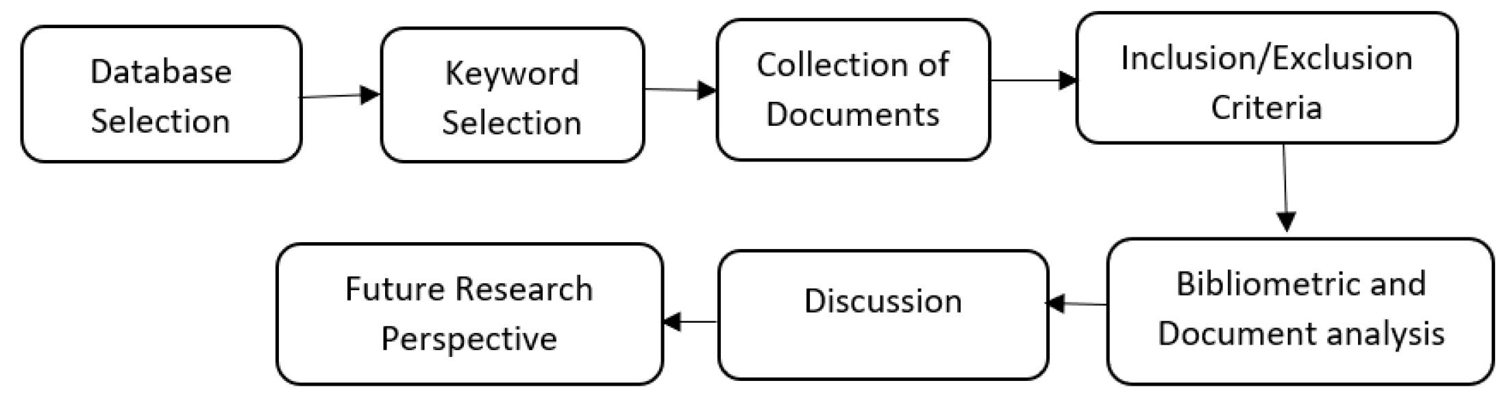
Figure 2.
Patent papers in scholar year (2020–2023).

Figure 3.
Citations papers in scholar year (2015–2023).

Figure 4.
Co-related keywords.

Figure 5.
Quantify bias in ML.

Figure 6.
Most common sources of bias.
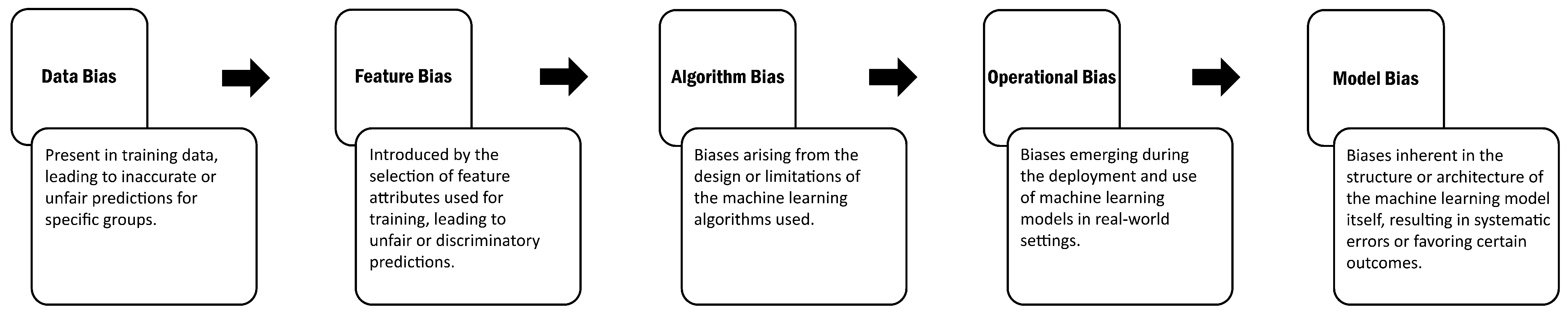
Figure 7.
Strategies of selection bias.

Figure 8.
Sample bias.

Figure 9.
Volunteer bias.

Figure 10.
Strategies for avoiding confirmation bias.

Figure 11.
Strategies to overcome confirmation bias.

Figure 12.
Types of algorithm bias.

Figure 13.
Adversarial training on NN.

Figure 14.
Causes of data bias.


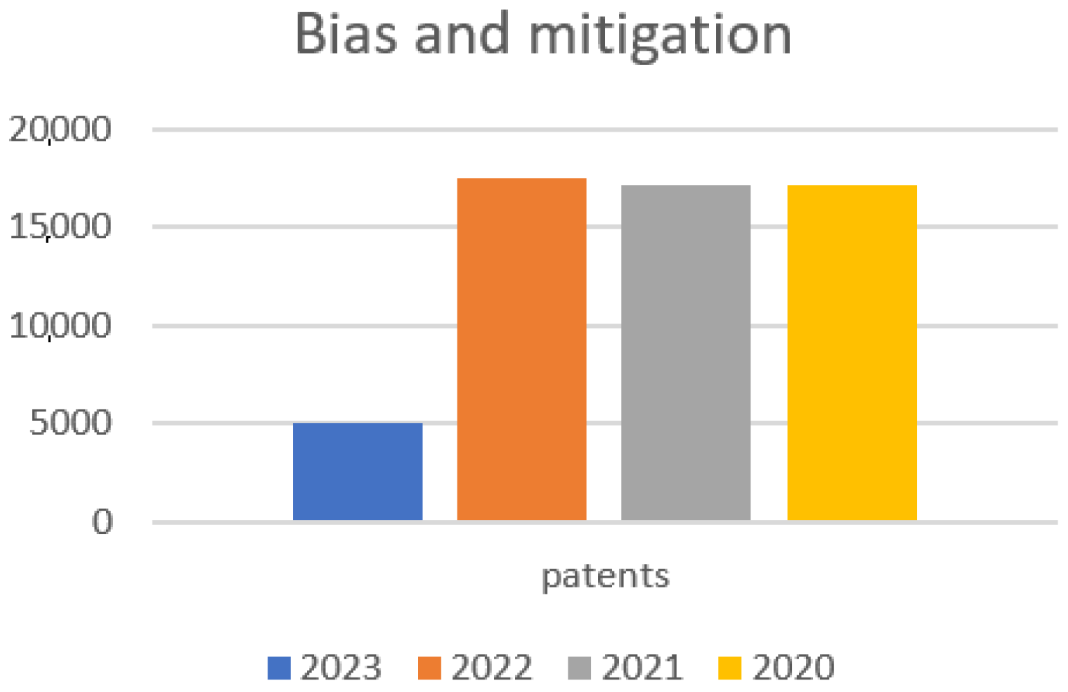
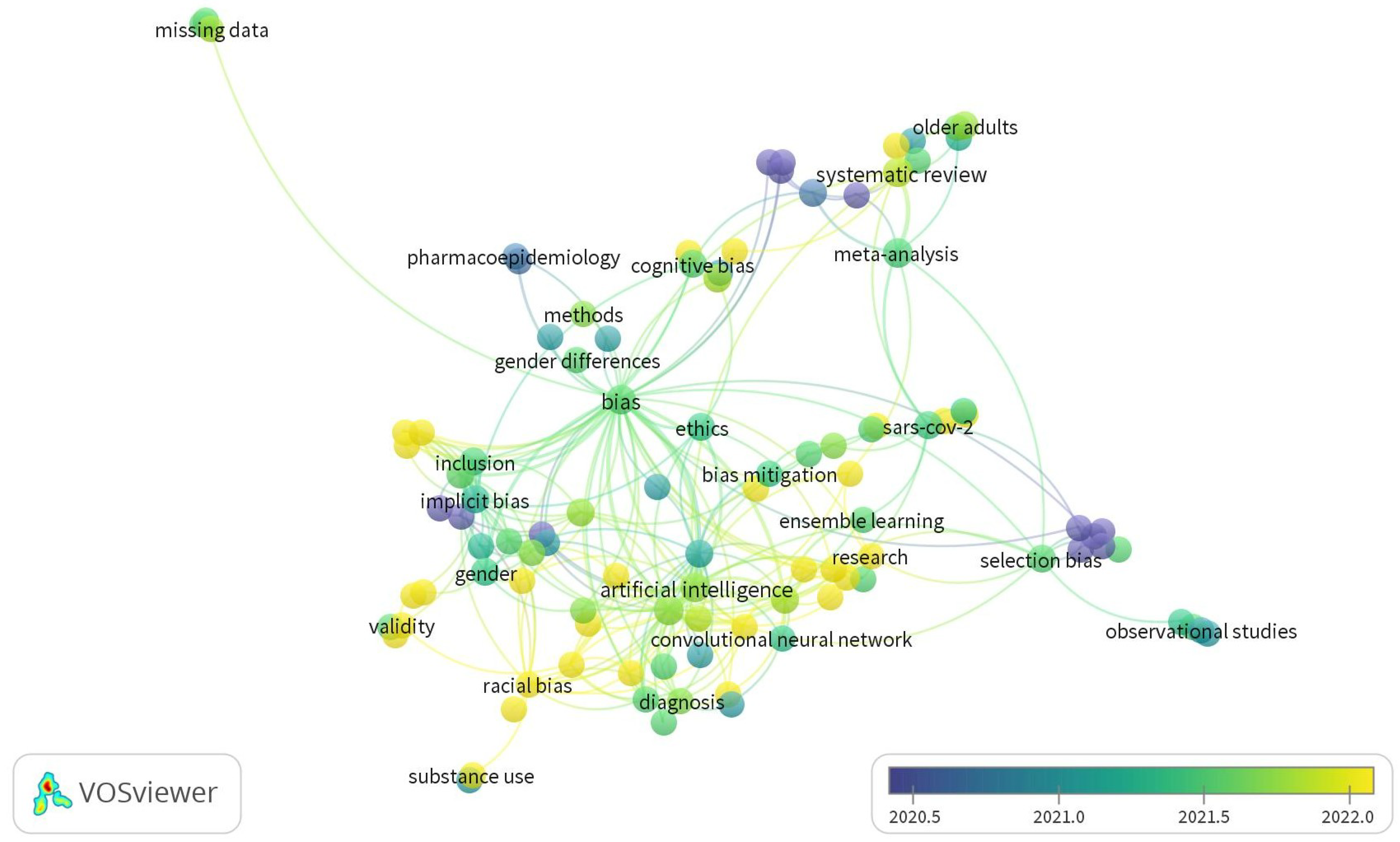
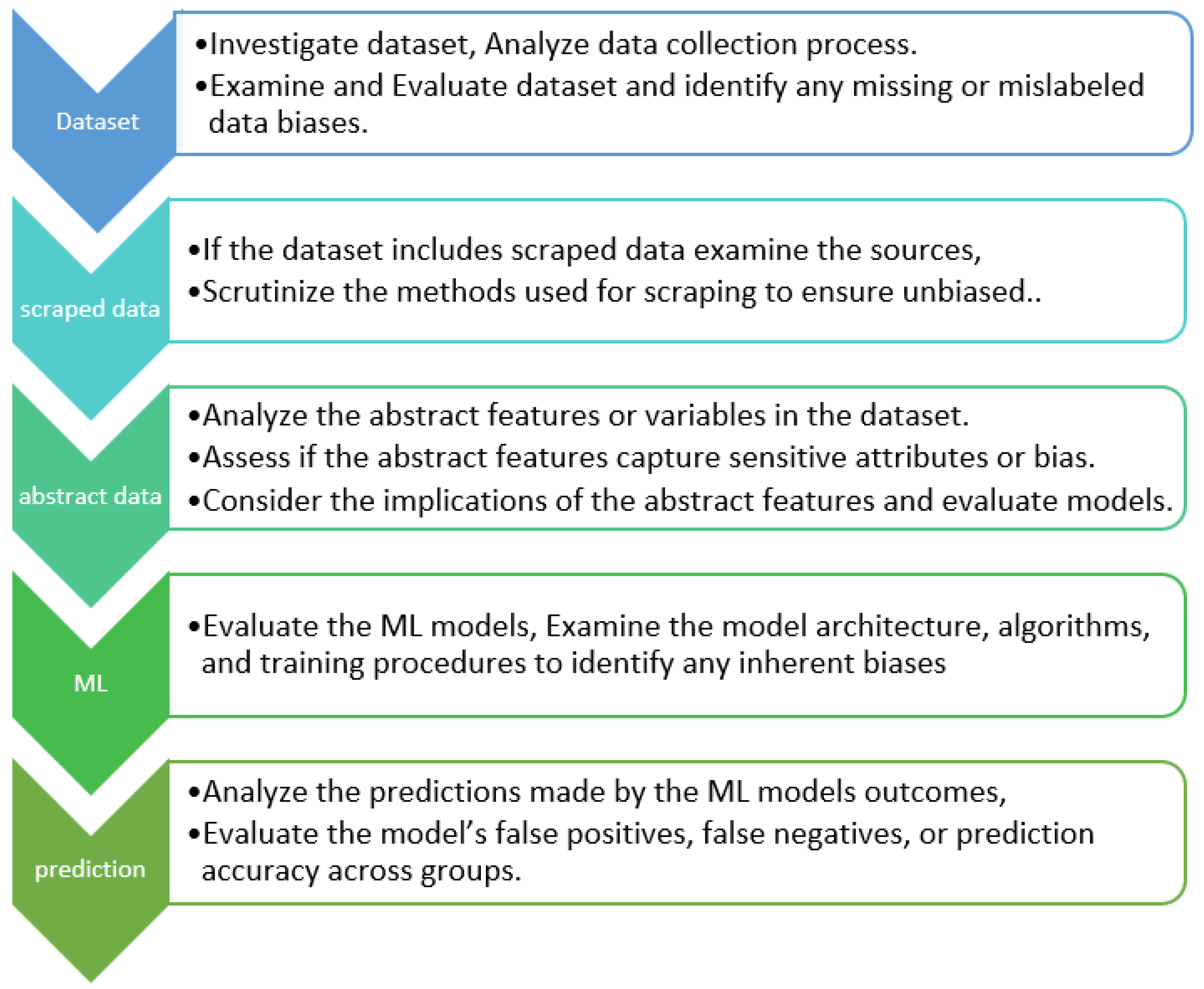
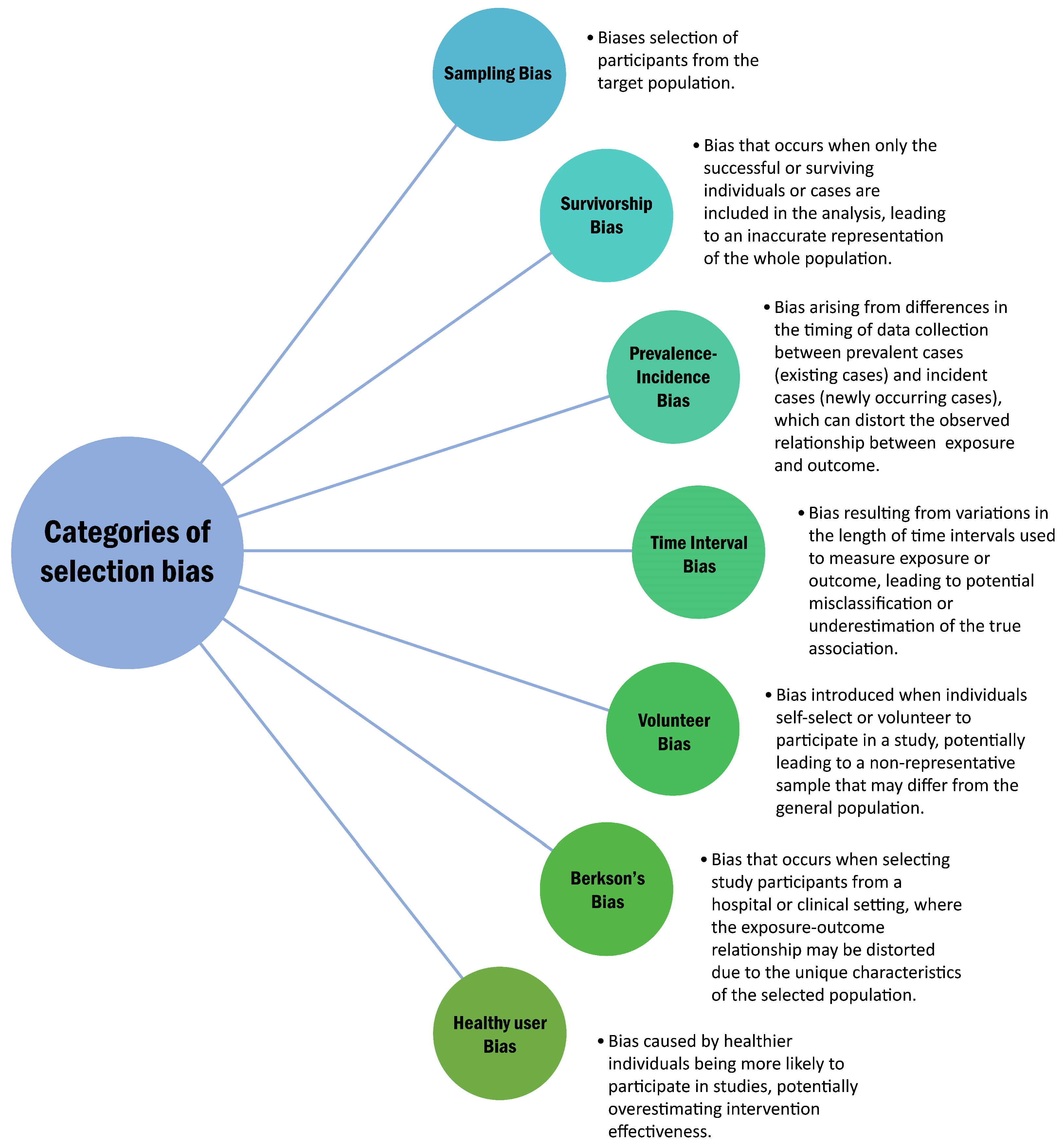
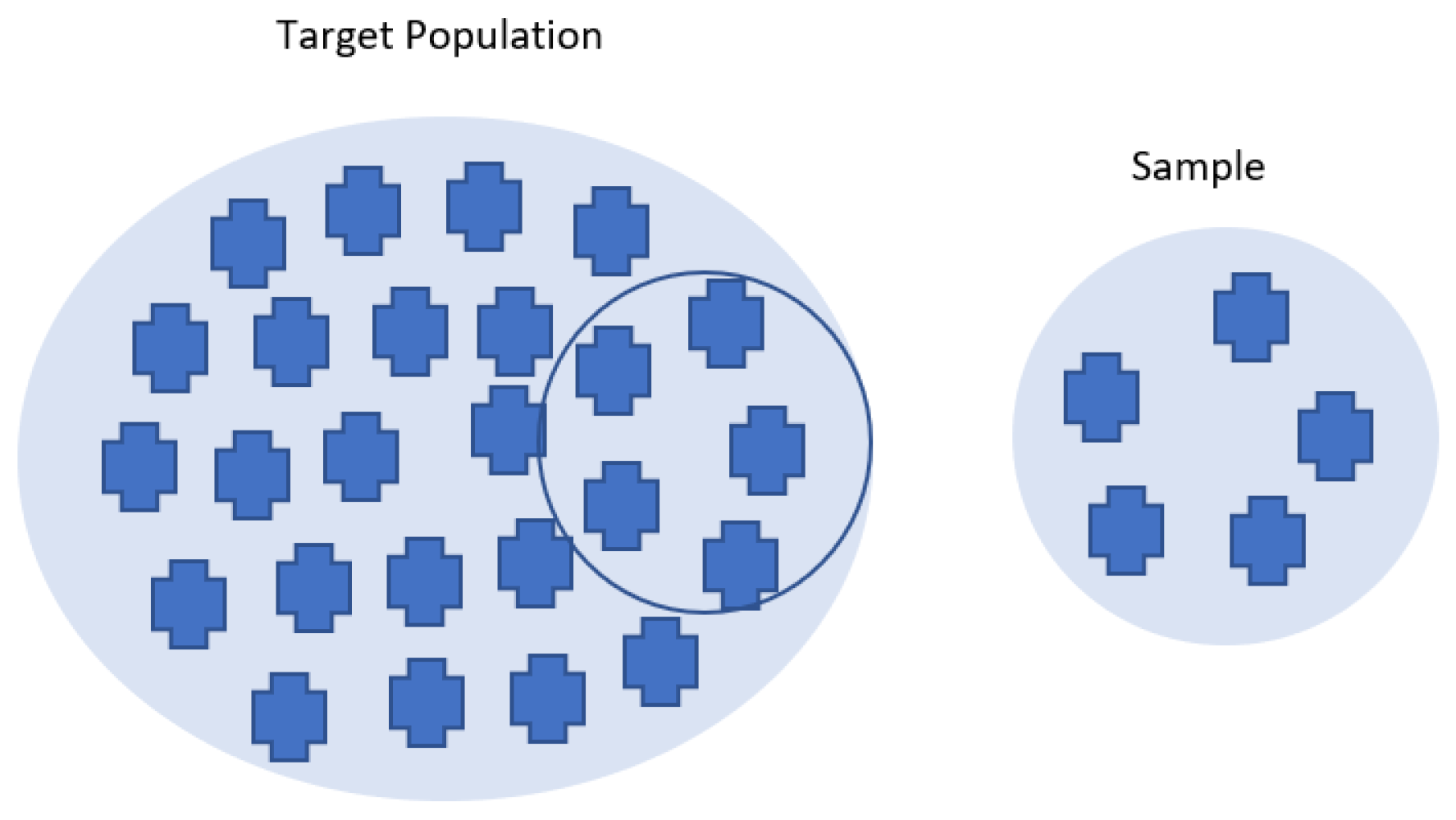
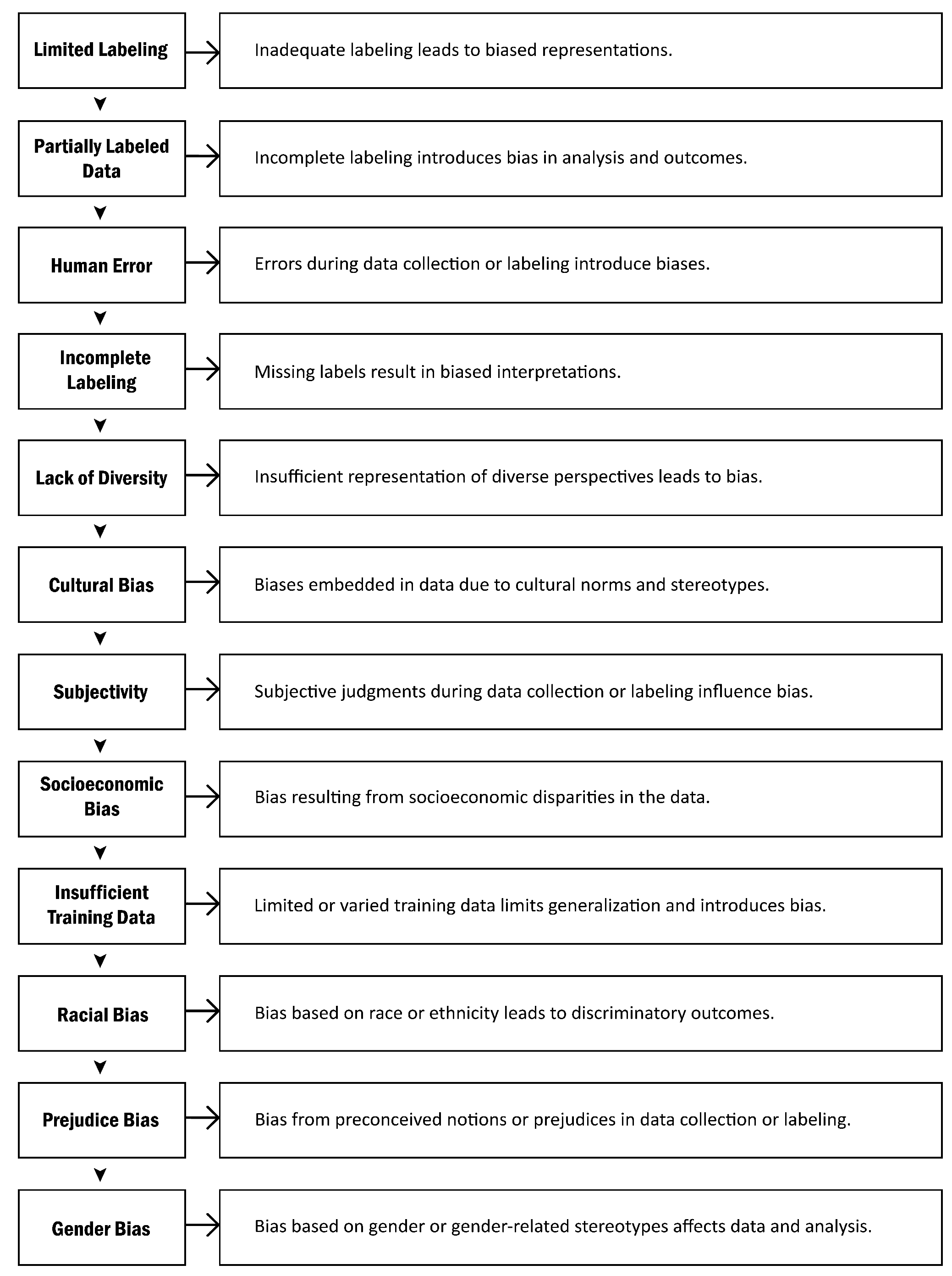
Table 1.
First search results (2023).
| Search Keyword | No. of Documents |
|---|---|
| “Machine learning bias” AND “mitigation” | 30 |
| “algorithmic bias ” OR “fairness in machine learning” | 1530 |
| “Unfairness model” OR “unintentional bias ” | 228 |
| “Ethical machine learning” AND “algorithmic transparency” | 3 |
| “Discrimination in machine learning” AND “counterfactual fairness” | 4 |
| “Bias in natural language processing” OR “fairness in text classification” | 133 |
| “Bias in computer vision” OR “fairness in image recognition” | 20 |
| Total | 1948 |
Table 2.
The most common sources of relevant published documents in 2023.
| Source | No. of Documents |
|---|---|
| Advances in Intelligent Systems and Computing (conference Proceedings) | 546 |
| Lecture Notes in Computer Science (conference Proceedings) | 6 |
| IEEE Access (conference Proceedings) | 1 |
| ACM International Conference Proceedings Series (survey) | 138 |
| International Journal of Production Research (Review article) | 49 |
| Computers and Industrial Engineering | 20 |
| CEUR Workshop Proceedings | 1 |
| IEEE Transactions on AI and Ethics | 82 |
| Machine Learning: A Multidisciplinary Approach (Springer) | 79 |
| Total | 922 |
Table 3.
Top 10 keywords.
| Source | No. of Occurrences |
|---|---|
| Bias | 45 |
| Machine Learning | 32 |
| Fairness | 9 |
| Mitigation measures | 4 |
| Algorithmic bias | 5 |
| bias mitigation | 5 |
| cognitive bias | 3 |
| Debiasing techniques | 2 |
| sampling bias | 5 |
| decision making process | 8 |
Table 4.
Summary of related work.
| Paper | Year | Contribution | Dataset | Limitation | Methods | Accuracy |
|---|---|---|---|---|---|---|
| Abay et al. [2] | 2020 | Framework both FL and fairness | Adult dataset, COMPAS | Focused only on binary classification but did not address biased data in FL on training data. | Local reweighing, global reweighing with privacy and federated bias removal. To mitigate bias pre-processing and in-processing methods. | Used 11.5% for fairness metrics and others use (FP, FN, curve) |
| Additional exploration of advanced techniques for bias detection and quantification, and impact of different types of biases on FL. | ||||||
| Zhenpeng et al. [8] | 2022 | Study (341 publications) on software engineering | Benchmark dataset, matrices, and benchmark | A limited set of bias mitigation techniques | Pre-processing, in-processing, and post-processing techniques | Revealing different methods and mitigating bias to predictive performance. |
| Future offerings, investigate methods and datasets, as well as exploring performance and fairness | ||||||
| Hort et al. [3] | 2022 | A systematic and extensive survey of various bias mitigation techniques. | 81 unique datasets. | Pre-processing, in-processing, and post-processing methods. | ML classifier | in-processing 212. |
| Future offerings, on bias mitigation techniques of three factors: metrics, benchmarking, and statistics. | ||||||
| Benjamin et al. [1] | 2022 | Comprehensive classification of machine learning biases and mitigation methods, highlighting potential pitfalls and perils of using algorithms. | Benchmarked | Focuses only business context | Six model-based methods used (bias removal approach, adversarial debiasing maximizes accuracy, Naive Bayes Classifiers, variable model, interpretable models, splitting and resampling | ML biases can be identified, avoided, and mitigated the CRISP-DM development process |
| Future offering: conversion of human biases into machine learning biases. | ||||||
| Lucas et al. [9] | 2022 | Measuring bias in text classification. | Hate Speech and Offensive Language dataset and Wikipedia Personal Attacks dataset. | Not suitable for limited diversity or representativeness | Statistical analysis and novel algorithm | Personal Attacks dataset, achieved 30% reduction maintain 90% predictive accuracy. Hate Speech and Offensive Language dataset, achieved a 13% reduction while maintaining 94% predictive accuracy. |
| Future offering: approach on larger and diverse datasets. | ||||||
| Zhixin et al. [10] | 2022 | Introduce a new attack model “neural Trojans”. Also proposed a new detection method on feature squeezing, to detect neural Trojans. | Does not use a dataset. | Not be effective against other types of AI Trojans | Demonstrate generative adversarial networks (GANs) | Demonstrates the feasibility of designing AI Trojans using GANs also propose a new detection method based on feature squeezing that are neural Trojans with high accuracy. |
| Future offering: detecting different types of AI Trojans. | ||||||
| Zhang et al. [11] | 2022 | Unbiased ML models in radiology by addressing the sources of bias | Dataset of chest X-rays | Lack of transparency regarding the dataset used in the case study. | Convolutional neural network (CNN) | AUC-ROC of 0.909 on the validation |
| Future offering: expanding the framework to other types of medical imaging or healthcare applications. | ||||||
| Korco et al. [4] | 2023 | Study of several bias mitigation approaches | Adult, Dutch, Compas, Bank, Credit | Not used on real-world datasets. Focused on a limited number of bias mitigation algorithms | Partial Least Squares Discriminant Analysis (PLS-DA) | Demographic parties and Equalized odds (Adult, Bank, COMPAS, Credit, Dutch-Biased 85.18, 73.74, 81.08, 83) |
| Future offering: developing more robust and fair bias mitigation algorithms. | ||||||
Table 5.
Analysis of the most relevant documents belonging to 2023.
| Reference | Topic | Limitation with Issues | Contribution |
|---|---|---|---|
| [12] | Bias and Unfairness in Machine Learning Models | Exploring multi-class and multi-metric characteristics is limited to binary approaches. | The work examines ML model fairness and bias reduction, emphasizing attribute concerns and transparency for fairer algorithms. |
| [13] | Variation of Gender Biases in Visual Recognition Models Before and After Fine-tuning | Pre-trained model biases and dataset size are poorly understood, according to the research. | Introduces image-based bias assessment for ML models. After extensive data fine-tuning, biases remain. To reduce downstream effects, it addressing fine-tuning biases. Bigger datasets may introduce and transmit bias. |
| [14] | A machine learning-based concentration-encoded molecular communication system | Numerical simulations are used without experimental validation. | Suggested technology reduces molecular communication bias and interference over current techniques. Longer transmission and 4-ary CPSK improve simulations. |
| [15] | Living with Floods Using State-of-the-Art and Geospatial Techniques | Lack of sufficient data, the Nonlinear relationship between causative factors and risk | A research employed ML to forecast floods and identify significant components. The best subtropical river basin model is ANN. A useful map for planning, prevention, and enforcement. |
| [16] | A Chinese Corpus For Gender Bias Probing and Mitigation | The use of highly educated gender-bias annotators may cause cognitive bias. Only a few Chinese language models were tested. Work should diversify annotators and investigate other models and solutions for their issues. | Created CORGI-PM, a 32.9 k-sentence dataset revealing Chinese gender prejudice. AI was challenged to identify and correct gender bias using several language models. This helps researchers discover and mitigate gender bias in Chinese literature. |
| [17] | Unveiling and Mitigating Bias in Ride-Hailing Pricing for Equitable Policy Making | Its focus on one city (Chicago) and the assumption that the government would subsidize discounts to make rides more affordable for disadvantaged residents. | It addresses ride-hailing price equity. It proposes fairness metrics pricing mechanisms and government subsidies. Practical experiments support ride-hailing policy improvements that promote fairness. |
Table 6.
Analysis of the most relevant documents belonging 2022.
| Reference | Topic | limitation with Issues | Contribution |
|---|---|---|---|
| [18] | An Investigation of Critical Issues in Bias Mitigation Techniques | The study evaluates 7 algorithms, image tasks, and biases. Identifies bias mitigation difficulties, pushing for wider examination and hidden biases. | Evaluation techniques are improved, bias reduction recommendations are proposed, and diverse architectures and structured concept-based predictions are suggested. |
| [19] | Data augmentation for fairness-aware machine learning | Focused on racial bias, overlooking gender and socioeconomic disparities. Data augmentation’s effectiveness varies with dataset variability, and detecting certain motions remains challenging. | The paper suggests fairness-aware ML for impartial law enforcement software. Data augmentation rebalances training data by race to reduce bias concerns without affecting data integrity. Real-world data experiments show balanced datasets may reduce law enforcement prejudice. |
| [20] | Auto-Debias: Debiasing Masked Language Models with Automated Biased Prompts | Proposed method solely debiases PLMs. Because big pre-trained language models are often used in real-world applications, reducing their human-like biases and societal preconceptions is crucial. | Auto-Debias reduces NLP bias efficiently and objectively. It reduces gender and racial biases in PLMs by automatically recognizing biased prompts, outperforming previous methods. This innovation advances NLP practical debiasing strategies. |
Table 7.
Analysis of the most relevant documents of 2021.
| Reference | Topic | limitation with Issues | Contribution |
|---|---|---|---|
| [21] | Mitigating bias in machine learning for medicine | Limited medical machine learning bias and patient outcome studies. Addressing bias essential for fair healthcare, advocating diverse data, robust model development, and careful clinical deployment. | Its integrative approach to building machine learning algorithms for medical applications provides concrete bias-reduction solutions. To provide equitable healthcare results, prejudice must be mitigated. |
| [22] | Debiasing Career Recommendations with Neural Fair Collaborative Filtering | Gender bias in career suggestions might dissuade women from STEM disciplines, hurting economic competitiveness and gender pay inequalities. NFCF reduces bias just for gender, according to the research. | NFCF combats gender bias in career recommender systems, according to the research. After pre-training and bias correction, it beats current models on MovieLens and Facebook datasets, potentially reducing gender salary gaps and STEM career discrepancies. |
| [23] | Evaluating causes of algorithmic bias in juvenile criminal recidivism | The research only included Catalan youth offenders, limiting its usefulness. Crime prediction using AI presents justice problems, especially for disadvantaged populations. Prediction accuracy and fairness are difficult to balance. | The research shows ML outperforms professional tools but favors certain populations. It pinpoints biases and offers solutions. Additionally, certain fairness approaches may have unintended bad effects. |
| [24] | Fairness metrics and bias mitigation strategies for rating predictions | The bias reduction strategy is designed for rating-based recommender systems and may not work for others. The evaluation is limited to two datasets, requiring more testing on other datasets for relevance. | The work innovates recommender system bias reduction and aligns fairness measures across domains. Recent findings emphasize bias reduction and fairness in algorithmic decision-making, particularly in recommenders. It helps reduce biases and improve fairness. |
| [25] | Detection and Evaluation of Bias in Machine Learning Models Using an Alternation Function | A single dataset with few gender and racial biases tests the study’s method. It needs further testing on varied datasets with different features. | The alternation function approach examines machine learning model bias for transparency and fairness. It focuses on detecting and quantifying human biases’ influence on ML through attribute value swaps. Practical model understanding and usefulness improve with this technique. |
Table 8.
Common sources of bias and their mitigation strategies.
| Bias Type | Definition | Example | Mitigation Strategies |
|---|---|---|---|
| Data Bias | Bias that arises from the quality, quantity, or representativeness of the training data | suppose a machine learning model is to predict whether a customer is likely to purchase a product based on their demographic and purchase history. We train the model on a dataset that consists of only men customers. The model performs well on this dataset, but when you apply it to a test dataset that includes women customers, it performs poorly. Then, the system is data in a bias phase. | Data augmentation, collecting diverse datasets, representativeness of training data |
| Feature Bias | Feature bias can arise from various sources such as incomplete data, selection bias, or pre-existing social biases. | For example, a company is building a machine learning model to predict whether a person is likely to default on a loan. They train the model on a dataset that includes features such as income, credit score, and employment history. However, they fail to include other relevant factors such as race, gender, or zip code, which can lead to biased predictions. In this case, feature bias arises. | Feature selection and pre-processing, careful consideration of feature choice, feature engineering to remove discriminatory features, dimensionality reduction |
| Model Bias | Model bias can arise from a variety of sources, including biased training data, biased algorithms, or biased human decisions that influence the design or implementation of the model. | Candidate’s height as a factor in hiring decisions can be an example of model bias. If height is used as a selection criteria, then it may disproportionately disadvantage shorter candidates, even if height is not a relevant factor for job performance. This bias can be perpetuated if the hiring team or the machine learning model has been trained on data that includes the height of successful candidates in the past. | Model Transparency and interpretability, regularized model training, model val- ideation and testing on diverse datasets |
| Algorithm Bias | Arises from the specific algorithm or optimization method used to train the machine learning model | Predicting flower species using ML could occur if the training dataset used to train the algorithm is biased towards certain types of flowers. if the training dataset contains mostly white flowers, the algorithm may have difficulty accurately predicting the species of flowers with different colors or shapes. This can result in the algorithm being biased towards certain types of flowers, which can lead to inaccurate predictions or misclassification of flowers. | Algorithmic auditing, hyperparameter tuning, and ensemble methods, fairness-aware algorithms, or optimization methods. |
| Operational Bias | Bias that arises from the deployment, usage, or interpretation of the machine learning model in real-world settings | Loan decisions can occur when the loan approval process relies too heavily on automated systems or algorithms that are not properly designed or tested. If the algorithm is not designed to account for all relevant factors, such as the credit history or employment status of the applicant, it may lead to inaccurate or biased loan decisions. To address operational bias in loan decisions, it is important to ensure that the loan application process is designed to minimize the potential for bias, and that loan officers and algorithms are trained and monitored to ensure they are making fair and objective decisions. | Regularly monitoring model performance and bias, introducing feedback mechanisms, ensuring ethical and responsible use of the model. |
Table 9.
Methods for minimizing sampling bias.
| Method | Details |
|---|---|
| Random sampling | Random sampling helps to ensure that every member of the population has an equal chance of being selected for the sample. This helps to prevent bias that can be introduced through non-random sampling techniques. |
| An increased sample size | larger sample size can help to reduce the impact of outliers and other anomalies that can introduce bias into the sample. However, it is important to ensure that the sample size is appropriate for the population being studied. |
| Use stratified sampling | Stratified sampling involves dividing the population into subgroups and then selecting a random sample from each subgroup. This can help to ensure that the sample includes representation from all subgroups, preventing bias that can be introduced through non-representative subgroups. |
| Be mindful of selection bias | Selection bias occurs when the sample is not representative of the population being studied. This can occur when the sample is self-selected or when the researcher selects participants based on certain characteristics. To minimize selection bias, it is important to use random sampling techniques and to ensure that the sample is diverse and representative of the population being studied. |
| Use a diverse sample | A diverse sample helps to ensure that the sample is representative of the population being studied. This can include diversity in terms of age, gender, race/ethnicity, education level, and other characteristics that may impact the results of the study. |
| Monitor participation rates | It is important to monitor participation rates to ensure that the sample is not biased towards those who are more likely to participate. This can help to prevent bias that can be introduced through non-response bias. |
Table 10.
Methods for minimizing volunteer bias.
| Method | Details |
|---|---|
| Random Selection | Select participants at random from the population to minimize the risk of bias. |
| Incentives | Offer incentives such as payment or a chance to win a prize to motivate more people to participate and reduce volunteer bias. |
| Masked Studies | Use a blinded or masked study design where participants do not know the true nature of the study to reduce self-selection bias. |
| Broad Advertising | Use of a variety of media outlets and advertising channels to reach a more diverse population and reduce volunteer bias. |
| Community Partnerships | Partner with community organizations to recruit participants and ensure that the study is representative of the community as a whole. |
Table 11.
Methods for minimizing survivorship bias.
| Method | Description |
|---|---|
| Use complete data | Collect and analyze data from all participants, including those who drop out or are lost to follow-up. |
| Impute missing data | Estimate missing data values based on patterns in the observed data, using methods such as mean imputation, regression imputation, or multiple imputation. |
| Sensitivity analysis | Assess of the robustness of the results by varying the assumptions about missing data, such as the degree of missing or the imputation method used. |
| Weighted analysis | Assign weights to each observation based on the probability of being observed, to adjust for differential attrition rates between groups. |
| Inverse probability weighting | Assign weights to each observation based on the inverse probability of being observed, to adjust for differential attrition rates between groups and the probability of missing. |
| Propensity score analysis | Use propensity scores to match or stratify participants based on their likelihood of being observed, to adjust for confounding factors and selection bias. |
Table 12.
Methods for minimizing time interval bias.
| Method | Description |
|---|---|
| Prospective study design | where outcomes are measured at the same time or at regular intervals over a specified period. |
| Matching outcome time intervals | Measuring outcomes to ensure that exposure status is accurately captured during the study period. |
| Statistical adjustment | Use statistical techniques such as time-dependent covariant analysis or survival analysis to adjust for changes in exposure status over time. |
| Sensitivity analysis | Perform sensitivity analyses to assess the impact of time interval bias on study results by varying the time intervals used to measure exposure and outcome. |
| Stratification | Stratify study participants based on exposure status and measure the outcome at specific time intervals for each group to identify any potential differences in the effect of exposure on the outcome over time. |
Table 13.
Methods for minimizing Berkson’s bias.
| Method | Description |
|---|---|
| Use a population-based sample | Select a sample of individuals from the general population, rather than from a specific group, such as those who are hospitalized or enrolled in a health program. |
| Control for confounding factors | Identify and control for other factors that could influence the relationship between the disease and the factor of interest. This can be performed through statistical techniques, such as multivariable regression analysis. |
| Use a randomized controlled trial | Randomly assign individuals to a treatment group or a control group, which can help minimize selection bias and other types of bias. |
| Use multiple recruitment sources | Recruit participants from multiple sources to avoid over-representation of individuals with a specific disease or condition. |
| Use clear inclusion and exclusion criteria | Develop clear criteria for inclusion and exclusion in the study to avoid selecting participants based on their disease status and other factors. |
Table 14.
Methods for minimizing prevalence–incidence bias.
| Method | Description |
|---|---|
| Defining the study population | Clearly define the study population and excluding individuals who have a long duration of the disease or condition being studied. This can help ensure that the denominator used to calculate incidence is accurate and not artificially inflated. |
| Identifying the time period | Clearly define the time period over which incidence is being measured. This can help to avoid including individuals who have had the disease or condition for a long time, which can inflate the prevalence and lead to an overestimation of incidence. |
| Adjusting for disease duration | Use statistical techniques to adjust for the duration of the disease or condition when estimating incidence. This can involve calculating incidence rates over shorter time intervals or using survival analysis techniques to adjust for the duration of the disease. |
| Conducting prospective studies | conducting prospective studies, which measure incidence over time, can help to minimize prevalence–incidence bias. In these studies, individuals are followed over time, and new cases of disease or condition are identified as they occur. |
Table 15.
Methods for minimizing selection bias.
| Method | Description |
|---|---|
| Use random sampling | Random sampling ensures that every member of the population has an equal chance of being selected for the study. This helps to ensure that the sample is representative of the population. |
| Use stratified sampling | Stratified sampling involves dividing the population into subgroups based on relevant characteristics, such as age, gender, or income level. Then, participants are randomly selected from each subgroup in proportion to their size in the population. This helps to ensure that the sample is representative of the population with respect to these important characteristics. |
| Use appropriate recruitment methods | To avoid self-selection bias need appropriate recruitment methods. For example, if the study aims to investigate the prevalence of a certain disease, researchers should not recruit participants from a hospital, as this will bias the sample towards those who are already sick. |
| Consider missing data | Missing data lead to selection bias. Estimate missing data or exclude participants with missing data only after examining whether their exclusion biases the sample. |
| Analyze and report sample characteristics | Analyze and report the characteristics of the sample including demographics and other relevant information. This helps to understand the representativeness of the sample and potential sources of bias. |
Table 16.
Mitigation of algorithm bias.
| Method | Description |
|---|---|
| Improving the quality and diversity of training data | One of the main causes of algorithm bias is flawed training data. By ensuring that the data used to train algorithms are representative of the real-world population and include diverse perspectives, biases can be minimized. |
| Using transparent and explainable algorithms | Algorithms that are transparent and explainable can help to identify and address bias more effectively. By providing clear insights into how the algorithm arrived at its results, it is easier to understand and address any biases that may be present. |
| Implementing regular audits and testing | Regular audits and testing can help to identify any biases in algorithms and ensure that they are producing fair and accurate results. This can involve analyzing the impact of the algorithm on different demographic groups and making adjustments as necessary. |
| Involving diverse stakeholders in the development process | Involving a diverse range of stakeholders in the development process, including those from under-represented groups, can help to identify and address potential biases before the algorithm is deployed. |
| Providing ongoing training and education | Providing ongoing training and education to those involved in the development and deployment of algorithms can help to raise awareness of algorithm bias and provide the skills and knowledge needed to prevent and mitigate it. |
Table 17.
Table of adversarial algorithms.
| Algorithm | Type | Description | Strengths | Weaknesses | Example |
|---|---|---|---|---|---|
| FGSM | Gradient-based | Computes the gradient of the loss function with respect to the input data and perturbs the data in the direction of the gradient. | Simple and fast; can generate effective adversarial examples. | May not generate robust adversarial examples that are resistant to other perturbation techniques. | Changing the label of an image from “dog” to “cat” by adding a small amount of noise. |
| PGD | Gradient-based | An iterative version of FGSM that applies small perturbations to the input data and projects the perturbed point onto a valid region of the input space. | Can generate more robust adversarial examples than FGSM; can be used to create multiple adversarial examples with varying degrees of distortion. | More computationally expensive than FGSM. | Generating an adversarial example that is misclassified as a stop sign instead of a yield sign. |
| CW attack | Optimization-based | Minimizes a custom loss function that encourages the perturbed input data point to be classified as the target label while minimizing the amount of perturbation. | Can generate adversarial examples that are difficult for a range of models to classify correctly; can generate adversarial examples with minimal perturbation. | Computationally expensive; may not always generate effective adversarial examples. | Generating an adversarial example that is misclassified as a “panda” instead of a “gibbon”. |
| DeepFool | Optimization-based | Iteratively finds the closest decision boundary to the input data point and perturbs the point in the direction of the boundary. | Can generate small perturbations that cause a misclassification; can generate adversarial examples that are difficult for the model to detect. | May not generate robust adversarial examples that are resistant to other perturbation techniques. | Changing the label of an image from “car” to “truck” by adding a small amount of noise. |
| JSMA | Gradient-based | Identifies the most important features of the input data point and perturbs them in a way that maximizes the model’s prediction error. | Can generate adversarial examples that are difficult for the model to classify correctly while minimizing the overall amount of perturbation. | May not generate robust adversarial examples that are resistant to other perturbation techniques. | Changing the label of an image from “bird” to “airplane” by perturbing the wings and beak of the bird. |
Table 18.
Some bias mitigation techniques in datasets.
| Technique | Description | Example |
|---|---|---|
| Data augmentation | Generate new data points by adding existing dataset. | Synthesize new data points for under-represented groups to increase dataset. |
| Balancing the dataset | Oversample the minority class or undersample the majority class to make the dataset more balanced | Undersample the majority group to balance the proportion of defaulters between the groups. |
| Feature engineering | Select and transform the input features used in model | Remove features that introduce bias, such as zip code, and add features that increase fairness, such as education level. |
| Regularization | Constrain the model’s parameters to prevent overfitting and encourage it to generalize better to new data | Add regularization terms to the loss function that encourage the model to use a wider range of features. |
| Counterfactual analysis | Identify scenarios and use them to test the model’s fairness | Simulate the effect of changing an applicant’s race or gender on the model’s prediction. |
| Fairness constraints | Constraints model ensure that it treats all groups fairly | Add a constraint that limits the difference in the model’s false positive rate between different racial groups. |
Disclaimer/Publisher’s Note: The statements, opinions and data contained in all publications are solely those of the individual author(s) and contributor(s) and not of MDPI and/or the editor(s). MDPI and/or the editor(s) disclaim responsibility for any injury to people or property resulting from any ideas, methods, instructions or products referred to in the content. |
© 2023 by the authors. Licensee MDPI, Basel, Switzerland. This article is an open access article distributed under the terms and conditions of the Creative Commons Attribution (CC BY) license (https://creativecommons.org/licenses/by/4.0/).
Share and Cite
MDPI and ACS Style
Siddique, S.; Haque, M.A.; George, R.; Gupta, K.D.; Gupta, D.; Faruk, M.J.H. Survey on Machine Learning Biases and Mitigation Techniques. Digital 2024, 4, 1-68. https://doi.org/10.3390/digital4010001
AMA Style
Siddique S, Haque MA, George R, Gupta KD, Gupta D, Faruk MJH. Survey on Machine Learning Biases and Mitigation Techniques. Digital. 2024; 4(1):1-68. https://doi.org/10.3390/digital4010001
Chicago/Turabian StyleSiddique, Sunzida, Mohd Ariful Haque, Roy George, Kishor Datta Gupta, Debashis Gupta, and Md Jobair Hossain Faruk. 2024. "Survey on Machine Learning Biases and Mitigation Techniques" Digital 4, no. 1: 1-68. https://doi.org/10.3390/digital4010001