Abstract
Land surface temperature (LST) is heavily influenced by urban morphology. Building height is an important parameter of urban morphology that affects LST. Existing studies show contradicting results where building height can have a positive or negative relationship with LST. More studies are necessary to examine the impact of building height. However, high accuracy building height data are difficult to obtain on a global scale and are not available in many places in the world. Using the Digital Building Height Model (DBHM) calculated by subtracting the SRTM from AW3D30, this study analyzes the relationship between building height and Landsat LST in two cities: Tokyo and Jakarta. The relationship is observed during both cities’ warm seasons (April to October) and Tokyo’s cool seasons (November to February). The results show that building height and LST are negatively correlated. In the morning, areas with high-rise buildings tend to have lower LST than areas with low-rise buildings. This phenomenon is revealed to be stronger during the warm season. The LST difference between low-rise and mixed-height building areas is more significant than between mixed-height and high-rise building areas.
1. Introduction
The exponential increase in urban population accompanied by the decreasing land availability has accelerated the pace of high-rise building constructions in the past few decades. One of the concerns with high-rise development is how it affects the urban climate. Urban heat island (UHI) has been a global issue [1] that is indicated by increasing land surface temperature (LST) [2]. Landsat LST has been widely used for monitoring UHI intensity because of its high availability in terms of spatial and temporal aspects. LST is reported to be strongly related to near-surface air temperature [3], and LST’s mean value at the city scale has good fittings with air temperature [4]. Existing studies show that LST is heavily influenced by urban morphology [5], such as building height [6], building density [7], building volume [8], and others. Building height is arguably the most important parameter of urban morphology that affects LST [6]. Studies have examined how building height affects LST and found contradicting results. Some studies suggested that higher buildings tend to have lower LST than low-rise buildings because of their large shadow [9], reflective roof materials [10], and air circulation around high-rise buildings [11]. However, other studies suggested that higher buildings tend to have higher LST because of large impervious surfaces [5] and high energy consumption for space cooling [12]. More studies to investigate the impact of building height on LST are required.
Building height data is crucial to investigate its relationship with LST. However, building height data at regional and global scales are limited [13]. The LiDAR method is popular for obtaining building height because it can produce high accuracies [14], but it involves complex data processing [15], requires high operational costs in data collection [16], and has limited access to the data. Due to these difficulties, LiDAR data are not available in many places of the world [17].
In the attempt to overcome the LiDAR limited availability, this study utilizes two satellite products, namely DSM (Digital Surface Model) from ALOS World 3D 30 m (AW3D30) and DEM (Digital Elevation Model) from Shuttle Radar Topographic Mission (SRTM). These two are widely used free global elevation datasets with the highest resolution available in Google Earth Engine (GEE) data catalog, which enables easy analysis at almost any place in the world. By subtracting SRTM from AW3D30, we can obtain the building height with a simple method and apply it to the LST analysis. This study defines the building height model obtained from that method as Digital Building Height Model (DBHM). Very few studies regard the difference between AW3D30 and SRTM as building height. Li et al. [13] used the building height obtained from AW3D30 and SRTM to compare to the building height obtained from Sentinel-1 data. The study found that DBHM has a correlation value of 0.60 with the reference height data at 500 m resolution [13]. Honjo et al. [18] applied moving averaging filters at DBHM, then examined the correlation of DBHM with LiDAR data. Visually, DBHM showed a good agreement with LiDAR data even before averaging, but the optimum correlation with LiDAR data was found after applying an averaging filter of 5 × 5 pixels (150 m × 150 m), which was 0.566 [18]. Considering the similarity between [DBHM and reference building height data presented in existing studies, DBHM is used in this paper.
Existing building height and LST studies mostly used LiDAR data in their research, limiting the study location to areas with access to LiDAR data. Using open DSMs data, we can analyze areas with no LiDAR data and support the lack of DBHM application in urban morphology and urban climate research. Hardly any studies have used DBHM to examine the impact of building height on LST. To the authors’ knowledge, only one study investigated the relationship between DBHM and LST of Landsat 8 in six global cities [19].
This study aims to analyze the relationship between building height and LST and resolve the contradictory research results using DBHM obtained from AW3D30 and SRTM by investigating two cities: Tokyo and Jakarta. Both have many high-rise building clusters in the central part of the city. In terms of climate, Tokyo is located in the warm temperate zone, while Jakarta is in the tropical rainforest zone [20,21]. The importance of both large metropolitan cities, the existence of high-rise clusters with different development levels, and contrasting climate conditions make these two cities intriguing to investigate. The cities are supported with sufficient cloud-free satellite data that makes the analysis possible. In this study, we use the LST of Landsat 5, acquired around 10 a.m. between 2006–2011, which coincides with the acquisition period of AW3D30. Further, we sample areas of different height classes to observe the impact of building height more closely, which was not conducted in the existing DBHM and LST study.
2. Materials and Methods
2.1. Study Areas
Tokyo, the capital city of Japan, and Jakarta, the capital of Indonesia, are metropolitan cities with numerous high buildings. Tokyo’s metropolitan area is the most populated area in the world, with a population of about 37 million people [22]. The first high-rise building in Tokyo, the 147 m-tall Kasumigaseki Building, was built in 1968, close to the center of Japan’s government bureaucracy. Later in the 1970s, a high-rise complex of more than 200 m-tall buildings was built in Shinjuku, along with Sunshine Building in Ikebukuro. These buildings signal the early state of high-rise building development in Tokyo. Among Tokyo’s buildings that exceed 150 m, 106 buildings were built between 1991 and 2011, and 86 of them were built between 2000 and 2011 [23].
Jakarta had a population of about over 10 million people in 2017, making it the largest megacity in Southeast Asia [24]. The first high-rise building in Jakarta was completed in 1967, the 74 m-tall Sarinah Retail Center. This building triggered the beginning of high-rise building development in Jakarta. The construction has continued since then, but the sudden increase in high-rise buildings in Jakarta happened after 1997. There were 22 high-rise buildings built between 1997 and 2007, and 42 high-rise buildings built between 2007 and 2017 [25].
The study areas are the center of Tokyo and Jakarta, where the high-rise clusters are located (Figure 1). Each urban area covers a rectangle of 0.1° (360 arc-seconds) in longitude and latitude. The size of an arc-second of latitude is constant, while the size of an arc-second of longitude decreases toward the earth’s poles.
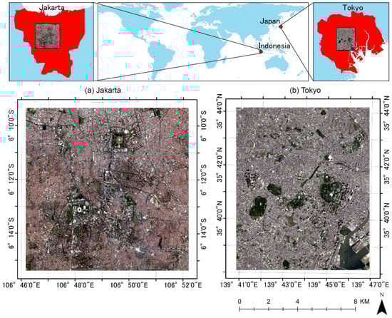
Figure 1.
Study area: (a) Jakarta and (b) Tokyo. The coverage in each area is 0.1° × 0.1° longitude and latitude. The size is different in meters.
2.2. Building Height Extraction
Two open access datasets are used to extract the building height information, AW3D30 and SRTM (Table 1). We generate the building height by subtracting SRTM from AW3D30, as the formula shown in Equation (1). The calculation method of DBHM in this paper is used in existing studies [13,18,19]. The AW3D30 and SRTM data of the defined study area are downloaded from Google Earth Engine (GEE) [26]. The data processing in this paper is conducted using programs written in R, a programming language for statistical computing [27]. Figure 2 shows the DBHM result calculated from Equation (1).

Table 1.
Datasets for building height extraction.
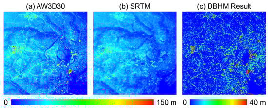
Figure 2.
Materials and extraction result of Digital Building Height Model in Tokyo. (a) AW3D30 minus (b) SRTM equals (c) DBHM result.
AW3D30 dataset was generated from stereo or triplet pair images obtained by the PRISM (Panchromatic Remote-sensing Instrument for Stereo Mapping) sensor aboard ALOS (Advanced Land Observing Satellite), operated by Japan Aerospace Exploration Agency. Approximately 3 million scenes were acquired from 2006 to 2011 to create fine-resolution DSM (5 m resolution) and ortho-rectified image (2.5 m resolution) [28]. The AW3D30 dataset was generated from the commercial AW3D 5 m mesh images, which were resampled to 30 m by averaging method, where the one-pixel value on AW3D30 is calculated from an average value of 7 by 7 pixels on AW3D 5 m [28]. The AW3D30 reportedly has a height accuracy of 4.40 m (root mean square error RMSE) globally [28]. Based on the land cover types, the RMSEs of AW3D30 range from 4.29 m in built-up areas to 6.75 m in dense vegetation areas [29].
SRTM data was produced from a joint project between NASA, the National Geospatial-Intelligence Agency, and the German and Italian Space Agencies. SRTM data was acquired in 2000 using Synthetic Aperture Radar (SAR) [30]. SRTM has a resolution of 1 arc-second (~30 m). The SRTM DSM has a height accuracy of 9.73 m (RMSE) globally [31]. Based on the land cover types, the RMSE ranges from 5.91 m in built-up areas to 10.42 m in bushland areas [29].
2.3. Land Surface Temperature Retrieval
Composites of Landsat 5 images from the U.S. Geological Survey from 2006 to 2011 were used to calculate LST. The period was chosen considering the acquisition period of AW3D30 data. The images were sorted by the clearest cloud coverage. Six images were picked for each season in Tokyo and five images were picked in Jakarta due to fewer clear days in Jakarta. The dates of images to create the LST maps are shown in Table 2. The selected dates fall from April to October for the warm season and from November to February for the cool season. Only a warm season is observed in Jakarta, considering the city has similar temperatures all year round. The surface temperature between land cover types in the warm season is more distinguishable compared to the cool season. The LST in this study refers to the urban surface temperature in the morning as the data are acquired around 10 a.m.
Table 2.
Analyzed Landsat 5 data.
The LST is calculated with the Statistical Mono-Window algorithm [32] using a GEE code repository provided by Ermida et al. [33]. The cloud mask processing is excluded due to the inaccurate removal of non-cloud coverages, such as bright roof surfaces. The images were then downloaded from GEE and composited. The composites were created based on the mean values of each area’s images to avoid the possible abnormality of a single LST date.
2.4. Vegetation and Water Coverages Removal
The vegetation and water coverages are removed from the analysis to minimize bias. Binary masks are created to locate vegetation and water coverages. The vegetation binary mask is created from Normalized Difference Vegetation Index (NDVI), and the water binary mask is created Normalized Difference Water Index (NDWI). Both indices are heavily influenced by temporal aspects and atmospheric conditions [34,35]. Hence, composite images were used to reduce the variability. The NDVI and NDWI are derived from the same Landsat images used for retrieving LST data.
NDVI values are obtained from the normalized difference between the near-infrared band (band 5 in Landsat 8) and the red band (band 4 in Landsat 8) of the TOA reflectance image. Meanwhile, the NDWI values are obtained from the normalized difference between the green band (band 3 in Landsat 8) and the near-infrared band. NDVI and NDWI range from −1.0 to +1.0. This study uses a threshold value of 0.4 for the NDVI and 0.1 for the NDWI to distinguish the coverages. The thresholds are decided after visual comparisons of the NDVI and NDWI maps and high-resolution images from Google Earth. Areas with values equal to or greater than the set thresholds are removed and not included in the analysis. Figure 3 illustrates how the water and vegetation masks are created by combining the NDVI and NDWI masks.
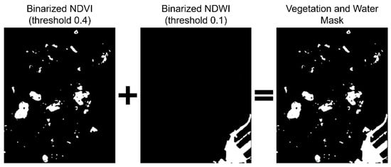
Figure 3.
Combining binarized NDVI and NDWI to create vegetation and water mask.
The formulas used to calculate the NDVI and NDWI [36] is shown in Equations (2) and (3), respectively.
where NIR (Near-Infrared reflectance) is Band 4, Red (red light reflectance) is Band 3, and Green (green light reflectance) is Band 2.
2.5. Relationship between Building Height and Land Surface Temperature
AW3D30, SRTM, and LST data are downloaded from GEE at the 30-m resolution, but the thermal band of Landsat-5 (LST data) originally had a spatial resolution of 120 m. A smoothing filter of window size 5 × 5 pixels is applied to the datasets to improve the spatial alignment between DBHM and LST. This filter results in one pixel having an average value of its surrounding 5 × 5 pixels. The illustration of the smoothing filter is shown in Figure 4.
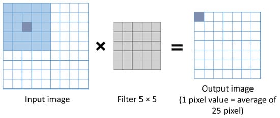
Figure 4.
Illustration of smoothing filter application.
After the images are averaged, we perform Pearson’s correlation and regression analysis to examine the relationship between building height and land surface temperature. Pearson’s correlation formula is shown in Equation (4), and the regression model follows Equation (5).
where is the Pearson’s correlation coefficient, is the DBHM, is the mean DBHM, is the LST, and is the mean LST.
where a is the coefficient, b is the intercept value, Y is the LST, and X is the DBHM.
3. Results
3.1. Spatial Distribution of Building Height and Land Surface Temperature
Figure 5 presents the distribution of DBHM and LST in Tokyo and Jakarta. Visually, the high DBHM area has lower LST than the low DBHM area. In both LST maps of Tokyo (Figure 5b,c), there is a large low LST area at the right part of the image, and at the same part in Tokyo DBHM (Figure 5a), the area appears to have many high buildings. These areas are Otemachi and Marunouchi business districts and major stations such as Shibuya, Shinjuku, and Ikebukuro. Tendencies are similar in the warm and cool season, but the cooling effect of high-rise buildings appear stronger during the warm season. For comparison, we picked three samples representing three height group areas, which are low-rise buildings, mixed-height buildings, and high-rise buildings areas. Each sample area is a size of 20 × 20 pixels (600 m× 600 m) and is marked with a square in Figure 5. Square H (high-rise) is located in the Marunouchi business district, Square M (mixed-height) is in the commercial area of Shibuya, and Square L (low-rise) is in the residential area of Toshima-ku.
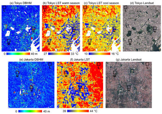
Figure 5.
Results of Digital Building Height Model and Land Surface Temperature. (a) Tokyo DBHM, (b) Tokyo LST warm season, (c) Tokyo LST cool season, (d) Tokyo Landsat, (e) Jakarta DBHM, (f) Jakarta LST, and (g) Jakarta Landsat. Square H: high-rise building area sample, Square M: mixed height building area sample, Square L: low-rise building area sample.
In Jakarta, a similar phenomenon is observed. The low LST area mostly belongs to the high DBHM area (Figure 5e,f). The low LST areas consist of the Sudirman Central Business District (SCBD), from the National Monument area in the north to the Senayan business district in the south. For the sample area in Jakarta, Square H is located inside SCBD, Square M is in Taman Anggrek, a complex of mixed-use high-rise buildings for shopping malls, apartments, and offices, and Square L is in a residential area in Kemayoran.
Figure 6 presents the graphs of mean building height and mean LST in each sampled area in both cities. There is a similar trend in both cities, where the low-rise building area has the highest mean LST, and the high-rise building area has the lowest LST. This further shows the trend of low LST in high-rise buildings area. During the warm season, the LST decrease in both cities is more significant from “low-rise” to “mixed-height” compared to “mixed-height” to “high-rise”. During the cool season in Tokyo, the LST decrease between each height class seems consistent, but overall, it is not as significant as in the warm season. In Tokyo (Figure 6a,b), the mean DBHM increase from low-rise to mixed-height is 3.17 m, and the LST decrease is 4.61 °C in the warm season and 2.12 °C in the cool season. Meanwhile, the mean DBHM increase from mixed-height to high-rise is 15.03 m, and the LST decrease is only 1.68 °C in the warm season and 1.63 12 °C in the cool season. In Jakarta (Figure 6c), the mean DBHM increase from low-rise to mixed-height is 6.77 m, and the LST decrease is 4.89 °C. Meanwhile, the mean DBHM increase from mixed-height to high-rise is 9.78 m, and the LST decrease is only 1.53 °C.
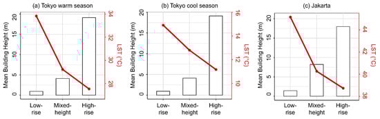
Figure 6.
Mean building height and mean LST of different sample areas in (a) Tokyo warm season, (b) Tokyo cool season, and (c) Jakarta.
3.2. Visualization of Land Surface Temperature on 3D Building Height Model
The 3D visualization presented in Figure 7 shows the mapped LST on the 3D building height model. The grey color is the removed vegetation and water area. Only the warm season in Tokyo is displayed due to the similar tendency. The high-rise buildings in Tokyo and Jakarta have different spatial distributions. In Tokyo, the high-rise buildings tend to clump together in several areas. Meanwhile, in Jakarta, the high-rise buildings areas are more solitary or form lines along major roads. Nonetheless, high-rise buildings in both cities form cooler areas than the surroundings.
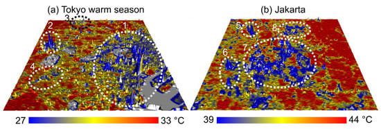
Figure 7.
Three-dimensional visualization of LST on building height model. Detected buildings appear as “spikes” in the model. Higher “spikes” means higher buildings. Circle 1–8 show high-rise areas with noticeable lower LST. (a) Tokyo warm season, (b) Jakarta.
In Tokyo (Figure 7a), Circle 1 is a large area of high-rise buildings, including Otemachi, Ginza, and Marunouchi. These areas are business and leisure districts that have many high-rise buildings. Circle 2 is a smaller clump of high-rise buildings in Shinjuku. The area is compact with high-rise buildings and has low LST. Circle 3 is Ikebukuro, and Circle 4 is Shibuya. The number of high-rise buildings in these areas is not as high as in Circle 1 and Circle 2, but the LST in these areas is visibly lower.
In Jakarta (Figure 7b), the high-rise buildings form many smaller clumps that are separated from each other. Areas with high-rise buildings have lower LST than areas only covered with low-rise buildings. The right part of the model, which is mostly covered with low-rise buildings, seems to have high LST. Some high-rise building areas are easily identified. Circle 5 is Taman Anggrek, a mixed-use buildings complex. Circle 6 is Permata Hijau shopping arcade & hotel and Pakubuwono apartment. Circle 7 is a combination of several business districts, such as Senayan, Sudirman, and Kuningan. Circle 8 is the National Monument that is surrounded by tall government offices.
From the 3D visualization of Tokyo and Jakarta, the building height models show the ability to detect major high-rise building areas. Further, the models show that the low LST area is spatially correlated with the high-rise buildings area.
3.3. Averaged Building Height and Land Surface Temperature
The moving average filter is applied to improve the spatial alignment between DBHM and LST map before the statistical analyses. Figure 8 shows the results of DBHM and LST after averaging with a window size of 5 × 5 pixels (150 m × 150 m). The tendency of high-rise building areas to have low LST can be observed clearer in the averaged version of LST and DBHM maps. Areas that appear cooler are areas that have higher DBHM. This tendency is weaker during the cool season.
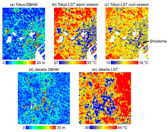
Figure 8.
The averaged version of (a) Tokyo digital building height model (DBHM), (b) Tokyo land surface temperature (LST) warm season, (c) Tokyo LST cool season, (d) Jakarta DBHM, and (e) Jakarta LST. In (a–c), the circled part is the Shiodome area that shows very high height values than in other areas.
The building height values decrease after the averaging process, but there is an area near Tokyo Bay, Shiodome, that exceedingly has higher values than other areas (marked in Figure 8). Shiodome is a redeveloped business and leisure city district near Tokyo Bay with many high-rise buildings. The present Shiodome was built after the year 2000.
3.4. Relationship between Averaged Land Surface Temperature and Building Height
Correlation and regression analyses are performed after the LST and DBHM are averaged. Based on the correlation analysis results, LST and DBHM have negative correlation coefficient values of −0.351 in Tokyo warm season, −0.348 in Tokyo cool season, and −0.315 in Jakarta. Both cities show p-values below 0.001, indicating that LST and building height are significantly correlated. The negative values show that there is a decrease in LST when there is an increase in building height. Areas covered with high-rise buildings tend to have lower LST than areas covered with low-rise buildings, showing that high-rise buildings have a cooling effect on the local surface temperature.
The regression analysis results are presented in Table 3. The results show that building height significantly affects LST in Tokyo and Jakarta. The scatterplot and boxplot diagrams in Figure 9 clearly show that the LST tends to decrease as the building height increases. Lower building classes, especially 0–10 m, have a wider range of LST. High-rise buildings seem to have a significant cooling effect within the height range of 0–20 m in both areas. After surpassing the 20 m class, the mean LST does not decrease significantly. It is worth noting that the height value is the height after averaging process with a window size of 150 × 150 m, which is lower than the actual building height. In the scatterplot of Jakarta, the highest value is about 100 m. Meanwhile, in Tokyo, although not many, some points surpassed 100 m. These values are detected in Shiodome, where the values are unusually higher than in other places.
Table 3.
Regression results of land surface temperature (LST) and digital building height model (DBHM). *** p-values less than 0.001.
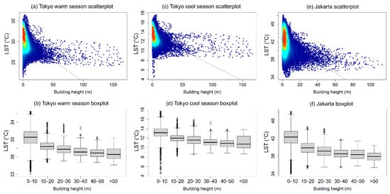
Figure 9.
Scatterplots and boxplots of the relationship between averaged LST and DBHM.
4. Discussion
According to the results, both Tokyo and Jakarta exhibit the same tendency, where high-rise building areas have lower LST than their surroundings. In Tokyo, many high-rise buildings tend to clump together in one area. Meanwhile, in Jakarta, the high-rise buildings are distributed along major roads, forming smaller clumps (Figure 7). Although high-rise buildings in Tokyo and Jakarta have different types of spatial distribution, both cities show that high-rise buildings have a cooling effect. The cooling effect of high-rise buildings has been observed in previous studies and an important factor that may cause it is building shadow [9,11]. Higher buildings cool the surface temperature by blocking solar radiation from reaching the ground [6]. They cast a larger shadow than lower buildings, potentially resulting in larger areas having lower LST.
It is worth noting that the cooling effect by high-rise buildings in this study is observed during daytime (around 10 a.m.), and it is likely not to be found during nighttime. Yang et al. [37] stated that the cooling effect, defined as the “urban cool island”, only lasts for several hours from the morning to noon. The study examined the phenomenon in Hong Kong that has compact high-rise buildings. Erell and Williamson [38] analyzed the diurnal and nocturnal pattern of urban heat islands in Adelaide, Australia, and found that there is an urban cool island phenomenon during daytime and an intense urban heat island during nighttime. The same study suggested that, during the day, lower buildings warm up faster than higher buildings, and during the night, lower buildings cool down faster than higher buildings, possibly due to different heat storage capacities [38].
The cooling effect in Tokyo appears in both warm and cool seasons. Although the effect is stronger in the warm season, this indicates that the cooling effect is not affected by seasonal variance. A study stated that the urban cool island could almost be found throughout the entire year, but it is stronger in summer [38]. This finding strengthens the possible role of a building’s heat storage capacity in forming an urban cool island.
The results show that the LST varies greatly in the low-rise building area (Figure 9). This phenomenon happens because the LST of low-rise buildings is found to be highly related to its neighboring landscape composition, such as pavements and vegetation [39]. A low-rise building near a vegetated area would likely have lower LST than a low-rise building near roads. As the building height increases, the effect of the surrounding landscape on the LST weakens. In addition, the results also reveal that the LST decrease from low-rise to mixed-height is more significant compared to mixed-height to high-rise. This finding should be of interest to urban planners in creating a mixed-height building composition, rather than a large low-rise composition, to alleviate high LST in an urban setting.
Figure 10 shows overlayed averaged DBHM map and LST map on the 3D building model of Google Earth in Shinjuku, Tokyo. The white color on DBHM and LST is the removed area because it is covered by vegetation, water, or the border pixels after the averaging process. The high-rise building complex in the middle forms a large cool area (Figure 10a). The LST difference between the high-rise building complex and its surrounding low-rise buildings is very distinguished. In low-rise building areas, there are extensive coverages of street surfaces. Meanwhile, in high-rise building areas, there are more coverages from wall and roof surfaces. A study [7] suggested that high-rise buildings have lower LST because the roof and wall surfaces can reflect radiation, and there is a smaller chance of radiation absorption.
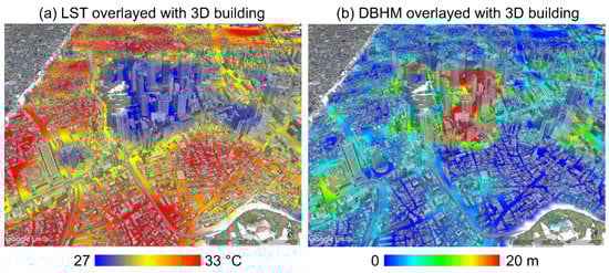
Figure 10.
Overlayed averaged (a) LST map and (b) DBHM map on the 3D building model of Shinjuku, Tokyo (Google Earth, Gray Buildings © 2022 ZENRIN).
Figure 10b shows that the DBHM corresponds well with high-rise buildings from the Google Earth 3D model. It also agrees well with the high LST area, as shown in Figure 10a. Existing studies that examined the relationship between building height and LST mostly used LiDAR data. Through this study, we exhibit the applicability of building height data obtained from open DSMs for studies related to LST. Currently, the DBHM is not validated with ground-truth data and cannot present accurate height values. It is only sufficient in showing the urban 3D structure information, especially for higher buildings. Since the data to extract DBHM are available in GEE and can be calculated simply, researchers from different backgrounds can utilize the DBHM easily. The possibility of deriving DBHM from another DEM, i.e., the Terra Advanced Spaceborne Thermal Emission and Reflection Radiometer (ASTER) Global Digital Elevation Map, should be evaluated for future study considering its equivalent spatial resolution to SRTM DEM.
The present study only analyzed the cooling effect during the daytime before noon and cannot consider the relationship between building height and urban surface temperature at different times of the day. High-rise buildings may have lower LST during the day and higher LST during the night. In addition, only building height is taken into consideration in this study, although the interaction of other factors, such as building density, building size or volume, etc., can also influence the LST. Future studies should consider current limitations to improve the research.
5. Conclusions
This study investigates the relationship between building height and land surface temperature using a digital building height model (DBHM) obtained from the difference between AW3D30 and SRTM in Tokyo and Jakarta. The results show that building height has a negative relationship with LST, whereas high-rise buildings tend to have low LST in the morning. The tendency is visible in both investigated areas regardless of their spatial distributions and different climate conditions. The cooling effect of high-rise buildings appears to exist throughout the year and is stronger during the warm season. The present study only observed the relationship in the morning, and the results are still deficient in explaining the phenomenon at different times of the day. However, it raises attention to building height considerations in urban planning.
This study is able to obtain building height information with a simple method and show the applicability of DBHM for urban climate study, which was barely utilized in existing studies. The DBHM extraction method is very simple and can be useful for future studies that require building height data but have technical and economic constraints. The produced building height model can detect the existence of mid-rise and high-rise buildings, although it does not measure the accurate building height. The findings of this study will hopefully be able to contribute to future studies that previously could not be conducted due to complex calculations in deriving the heights of buildings. Practically, this study could add some consideration to the urban planning sector to create a space where the building height is not uniform because a mixed-height area could significantly decrease LST.
Author Contributions
Conceptualization, D.D. and T.H; methodology, T.H. and D.D.; writing—original draft preparation, D.D.; writing—review and editing, T.H., K.F.; visualization, D.D. All authors have read and agreed to the published version of the manuscript.
Funding
This research received no external funding.
Data Availability Statement
Not applicable.
Acknowledgments
The authors thank Akira Kato for helpful feedback on the initial manuscript.
Conflicts of Interest
The authors declare no conflict of interest.
References
- Filho, W.L.; Wolf, F.; Castro-Díaz, R.; Li, C.; Ojeh, V.; Gutiérrez, N.; Nagy, G.; Savić, S.; Natenzon, C.; Al-Amin, A.Q.; et al. Addressing the urban heat islands effect: A cross-country assessment of the role of green infrastructure. Sustainability 2021, 13, 753. [Google Scholar] [CrossRef]
- Galodha, A.; Gupta, S.K. Land surface temperature as an indicator of urban heat island effect: A google earth engine based Web-App. Int. Arch. Photogramm. Remote Sens. Spat. Inf. Sci. ISPRS Arch. 2021, 44, 57–62. [Google Scholar] [CrossRef]
- Good, E.J.; Ghent, D.J.; Bulgin, C.E.; Remedios, J.J. A spatiotemporal analysis of the relationship between near-surface air temperature and satellite land surface temperatures using 17 years of data from the ATSR series. J. Geophys. Res. Atmos. 2017, 122, 9185–9210. [Google Scholar] [CrossRef]
- Sun, T.; Sun, R.; Chen, L. The trend inconsistency between land surface temperature and near surface air temperature in assessing Urban heat island effects. Remote Sens. 2020, 12, 1271. [Google Scholar] [CrossRef]
- Cai, M.; Ren, C.; Xu, Y.; Lau, K.K.L.; Wang, R. Investigating the relationship between local climate zone and land surface temperature using an improved WUDAPT methodology–A case study of Yangtze River Delta, China. Urban Clim. 2018, 24, 485–502. [Google Scholar] [CrossRef]
- Zheng, Z.; Zhou, W.; Yan, J.; Qian, Y.; Wang, J.; Li, W. The higher, the cooler? Effects of building height on land surface temperatures in residential areas of Beijing. Phys. Chem. Earth 2019, 110, 149–156. [Google Scholar] [CrossRef]
- Yang, X.; Li, Y. The impact of building density and building height heterogeneity on average urban albedo and street surface temperature. Build. Environ. 2015, 90, 146–156. [Google Scholar] [CrossRef]
- Alavipanah, S.; Schreyer, J.; Haase, D.; Lakes, T.; Qureshi, S. The effect of multi-dimensional indicators on urban thermal conditions. J. Clean. Prod. 2018, 177, 115–123. [Google Scholar] [CrossRef]
- Nichol, J.E. High-resolution surface temperature patterns related to urban morphology in a tropical city: A satellite-based study. J. Appl. Meteorol. 1996, 35, 135–146. [Google Scholar] [CrossRef]
- Honjo, T.; Tsunematsu, N.; Yokoyama, H.; Yamasaki, Y.; Umeki, K. Analysis of urban surface temperature change using structure-from-motion thermal mosaicing. Urban Clim. 2017, 20, 135–147. [Google Scholar] [CrossRef]
- Wang, M.; Xu, H. The impact of building height on urban thermal environment in summer: A case study of Chinese megacities. PLoS ONE 2021, 16, e0247786. [Google Scholar] [CrossRef] [PubMed]
- Guo, G.; Zhou, X.; Wu, Z.; Xiao, R.; Chen, Y. Characterizing the impact of urban morphology heterogeneity on land surface temperature in Guangzhou, China. Environ. Model. Softw. 2016, 84, 427–439. [Google Scholar] [CrossRef]
- Li, X.; Zhou, Y.; Gong, P.; Seto, K.C.; Clinton, N. Developing a method to estimate building height from Sentinel-1 data. Remote Sens. Environ. 2020, 240, 111705. [Google Scholar] [CrossRef]
- National Oceanic and Atmospheric Administration (NOAA) Coastal Services Center. Lidar 101: An Introduction to Lidar Technology, Data, and Applications; NOAA Coastal Service Center: Charleston, SC, USA, 2012; p. 76. [Google Scholar]
- Hummel, S.; Hudak, A.T.; Uebler, E.H.; Falkowski, M.J.; Megown, K.A. A comparison of accuracy and cost of LiDAR versus stand exam data for landscape management on the Malheur National Forest. J. For. 2011, 109, 267–273. [Google Scholar]
- Bi, S.; Yuan, C.; Liu, C.; Cheng, J.; Wang, W.; Cai, Y. A survey of low-cost 3D laser scanning technology. Appl. Sci. 2021, 11, 3938. [Google Scholar] [CrossRef]
- Alobeid, A.; Jacobsen, K.; Heipke, C. Comparison of matching algorithms for DSM generation in urban areas from Ikonos imagery. Photogramm. Eng. Remote Sens. 2010, 76, 1041–1050. [Google Scholar] [CrossRef]
- Honjo, T.; Danniswari, D.; Seo, Y.; Tsunematsu, N.; Yokoyama, H. Simple Method for Detecting Urban 3D Structure Using Open-Source Satellite Data. 2022; Manuscript submitted for publication. [Google Scholar]
- Danniswari, D.; Honjo, T.; Kato, A.; Furuya, K. Utilizing Open-Source Satellite Data for the Relationship between Building Height and Land Surface Temperature. J. Environ. Inf. Sci. 2021, 2021, 1–10. [Google Scholar] [CrossRef]
- Kottek, M.; Grieser, J.; Beck, C.; Rudolf, B.; Rubel, F. World map of the Köppen-Geiger climate classification updated. Meteorol. Z. 2006, 15, 259–263. [Google Scholar] [CrossRef]
- Richards, D.; Masoudi, M.; Oh, R.R.Y.; Yando, E.S.; Zhang, J.; Friess, D.A.; Grêt-Regamey, A.; Tan, P.Y.; Edwards, P.J. Global variation in climate, human development, and population density has implications for urban ecosystem services. Sustainability 2019, 11, 6200. [Google Scholar] [CrossRef]
- United Nations, Department of Economic and Social Affairs. The World ’s Cities in 2018; United Nations: New York, NY, USA, 2018; p. 34. [Google Scholar]
- Perez, R.I.P. The historical development of the Tokyo skyline: Timeline and morphology. J. Asian Arch. Build. Eng. 2014, 13, 609–615. [Google Scholar] [CrossRef][Green Version]
- Wandira, P.A.; Jongwook, K. The Influence of Tall Buildings to the Modern Urban Landscape of Jakarta City. In Proceedings of the UIA 2017 Seoul World Architects Congress, Seoul, Korea, 3–10 September 2017; pp. 0–6. [Google Scholar]
- Effendi, M.F.; Ridzqo, I.F.; Dharmatanna, S.W. An Overview of High-Rise Buildings in Jakarta since 1967 to 2020. IOP Conf. Ser. Earth Environ. Sci. 2021, 933, 012001. [Google Scholar] [CrossRef]
- Gorelick, N.; Hancher, M.; Dixon, M.; Ilyushchenko, S.; Thau, D.; Moore, R. Google Earth Engine: Planetary-scale geospatial analysis for everyone. Remote Sens. Environ. 2017, 202, 18–27. [Google Scholar] [CrossRef]
- R Core Team. R: A Language and Environment for Statistical Computing; R Foundation for Statistical Computing: Vienna, Austria, 2020; Available online: https://www.R-project.org/ (accessed on 11 April 2022).
- Tadono, T.; Nagai, H.; Ishida, H.; Oda, F.; Naito, S.; Minakawa, K.; Iwamoto, H. Generation of the 30 M-MESH global digital surface model by alos prism. Int. Arch. Photogramm. Remote Sens. Spat. Inf. Sci. ISPRS Arch. 2016, 41, 157–162. [Google Scholar] [CrossRef]
- Santillan, J.R.; Makinano-Santillan, M. Vertical accuracy assessment of 30-M resolution ALOS, ASTER, and SRTM global DEMS over Northeastern Mindanao, Philippines. Int. Arch. Photogramm. Remote Sens. Spat. Inf. Sci. ISPRS Arch. 2016, 41, 149–156. [Google Scholar] [CrossRef]
- Farr, T.G.; Rosen, P.A.; Caro, E.; Crippen, R.; Duren, R.; Hensley, S.; Kobrick, M.; Paller, M.; Rodriguez, E.; Roth, L.; et al. The Shuttle Radar Topography Mission. Rev. Geophys. 2007, 45, RG2004. [Google Scholar] [CrossRef]
- Mukul, M.; Srivastava, V.; Jade, S.; Mukul, M. Uncertainties in the Shuttle Radar Topography Mission (SRTM) Heights: Insights from the Indian Himalaya and Peninsula. Sci. Rep. 2017, 7, 41672. [Google Scholar] [CrossRef] [PubMed]
- Hulley, G.; Shivers, S.; Wetherley, E.; Cudd, R. New ECOSTRESS and MODIS land surface temperature data reveal fine-scale heat vulnerability in cities: A case study for Los Angeles County, California. Remote Sens. 2019, 11, 2136. [Google Scholar] [CrossRef]
- Ermida, S.L.; Soares, P.; Mantas, V.; Göttsche, F.M.; Trigo, I.F. Google earth engine open-source code for land surface temperature estimation from the landsat series. Remote Sens. 2020, 12, 1471. [Google Scholar] [CrossRef]
- El-Gammal, M.I.; Ali, R.R.; Samra, R.M.A. NDVI Threshold Classification for Detecting Vegetation Cover in Damietta Governorate, Egypt. J. Am. Sci. 2014, 10, 108–113. [Google Scholar] [CrossRef]
- Liu, Y. Why NDWI threshold varies in delineating water body from multitemporal images? In Proceedings of the 2012 IEEE International Geoscience and Remote Sensing Symposium, Munich, Germany, 22–27 July 2012; pp. 4375–4378. [Google Scholar] [CrossRef]
- McFeeters, S.K. The use of the Normalized Difference Water Index (NDWI) in the delineation of open water features. Int. J. Remote Sens. 1996, 17, 1425–1432. [Google Scholar] [CrossRef]
- Yang, X.; Li, Y.; Luo, Z.; Chan, P.W. The urban cool island phenomenon in a high-rise high-density city and its mechanisms. Int. J. Clim. 2017, 37, 890–904. [Google Scholar] [CrossRef]
- Erell, E.; Williamson, T. Intra-urban differences in canopy layer air temperature at a mid-latitude city. Int. J. Clim. 2006, 27, 1243–1255. [Google Scholar] [CrossRef]
- Feng, X.; Myint, S.W. Exploring the effect of neighboring land cover pattern on land surface temperature of central building objects. Build. Environ. 2016, 95, 346–354. [Google Scholar] [CrossRef]
Publisher’s Note: MDPI stays neutral with regard to jurisdictional claims in published maps and institutional affiliations. |
© 2022 by the authors. Licensee MDPI, Basel, Switzerland. This article is an open access article distributed under the terms and conditions of the Creative Commons Attribution (CC BY) license (https://creativecommons.org/licenses/by/4.0/).