
Photogrammetry from UAV and Low-Cost Lidar for Sinkhole Hazard Mitigation in Urban Areas: Applications and Evaluations

Abstract
:1. Introduction
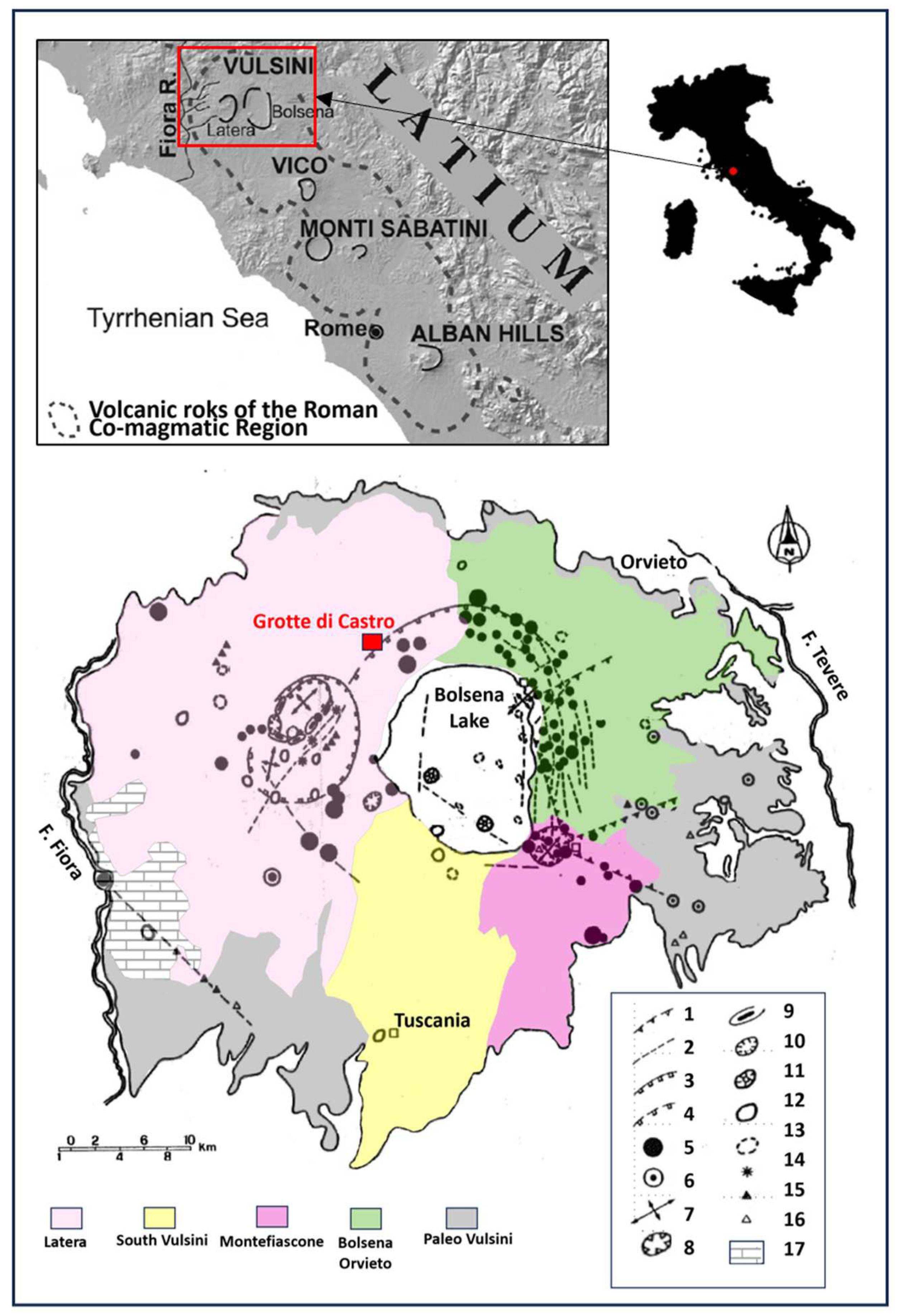
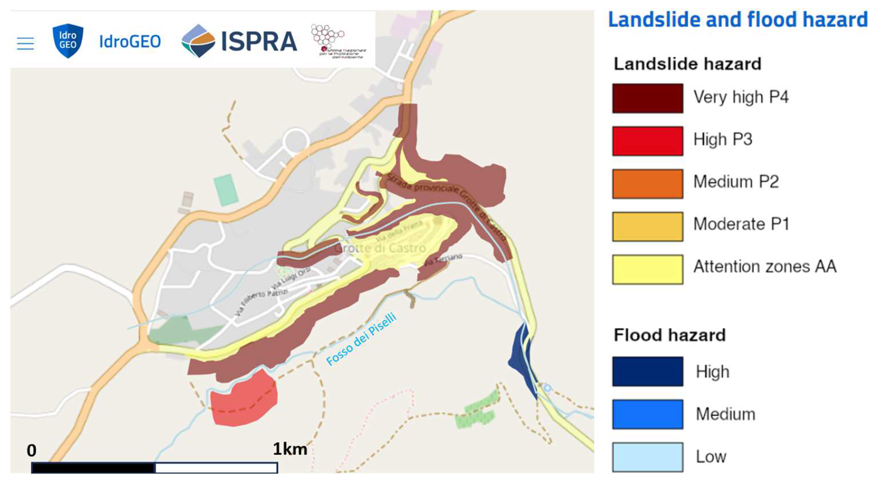
2. Study Area
2.1. Geological Context
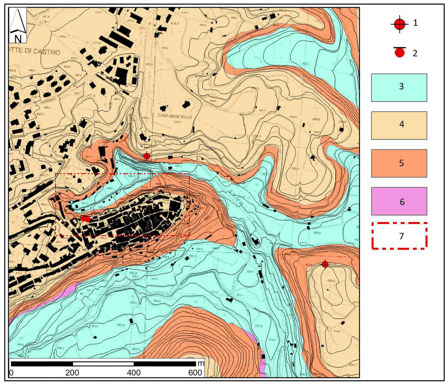
2.2. Geomorphological and Stratigraphic Setting
3. Materials and Methods
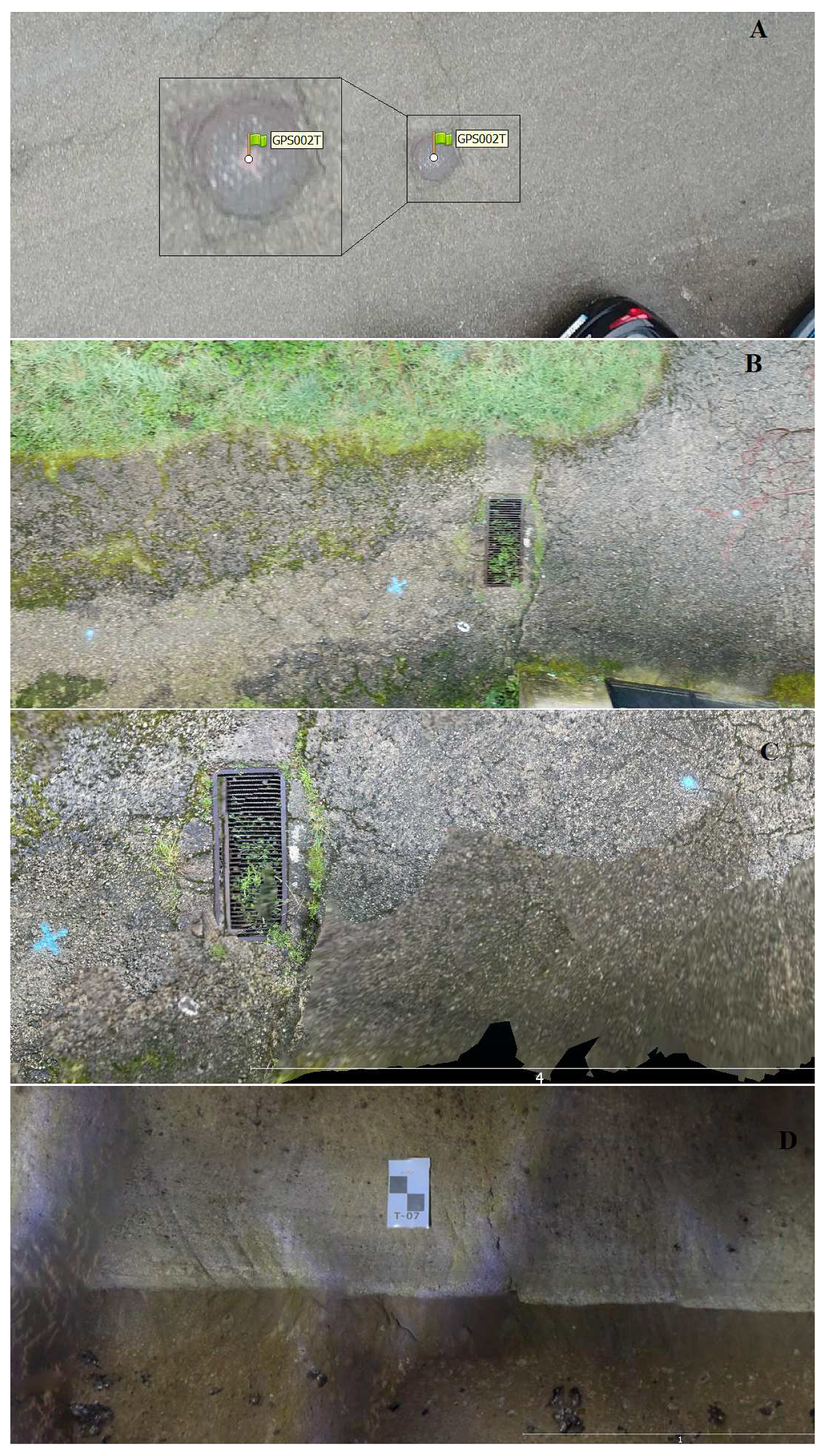
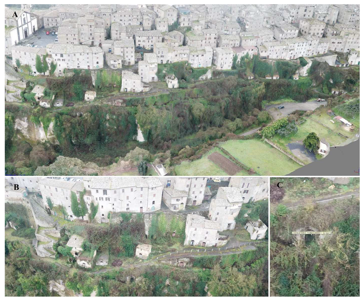
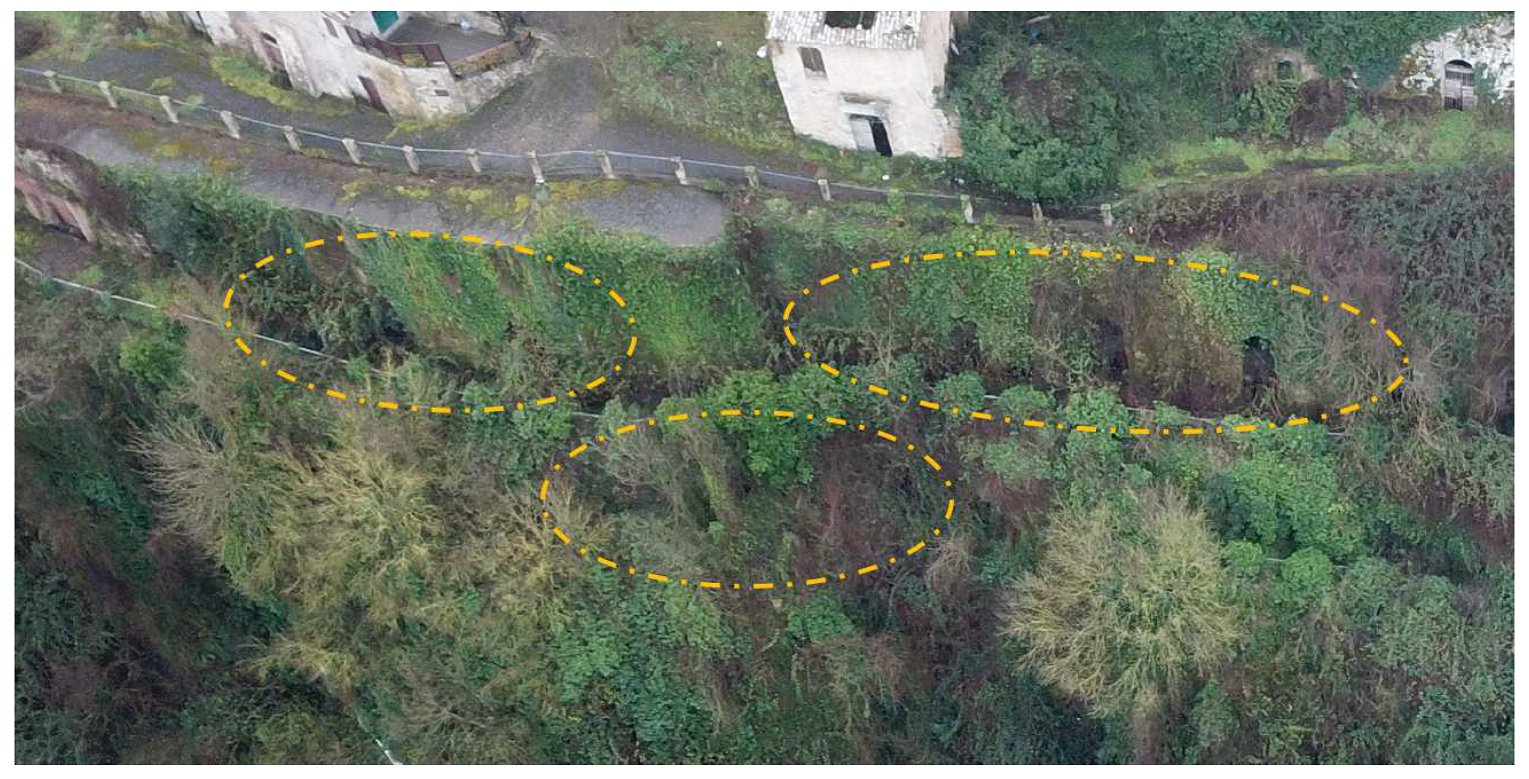
3.1. Photogrammetric Surveys
3.2. Lidar Surveys and Traditional Surveys
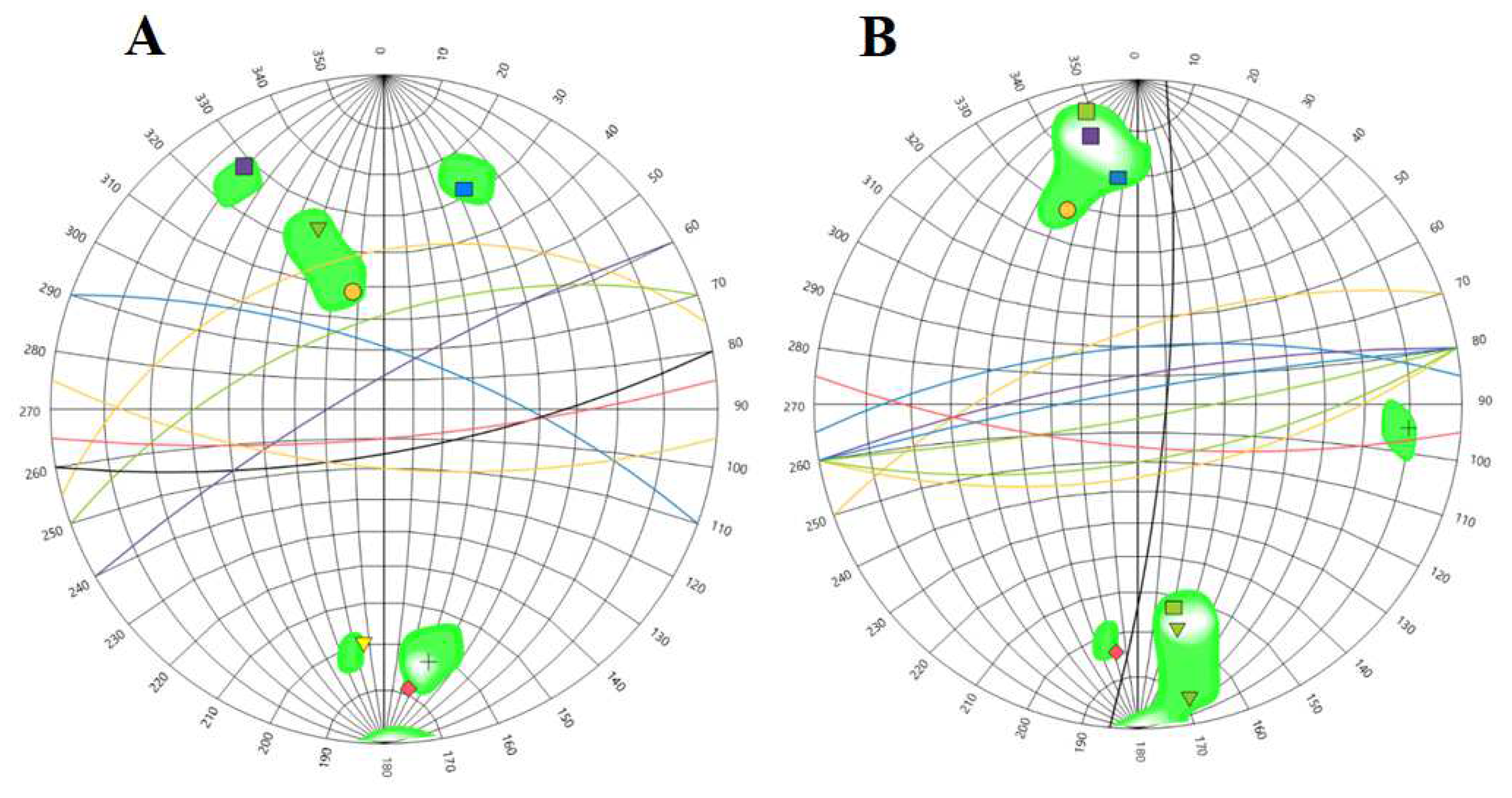
3.3. Geomechanical Survey
3.4. Basic Methods for Stability Assessment
4. Results
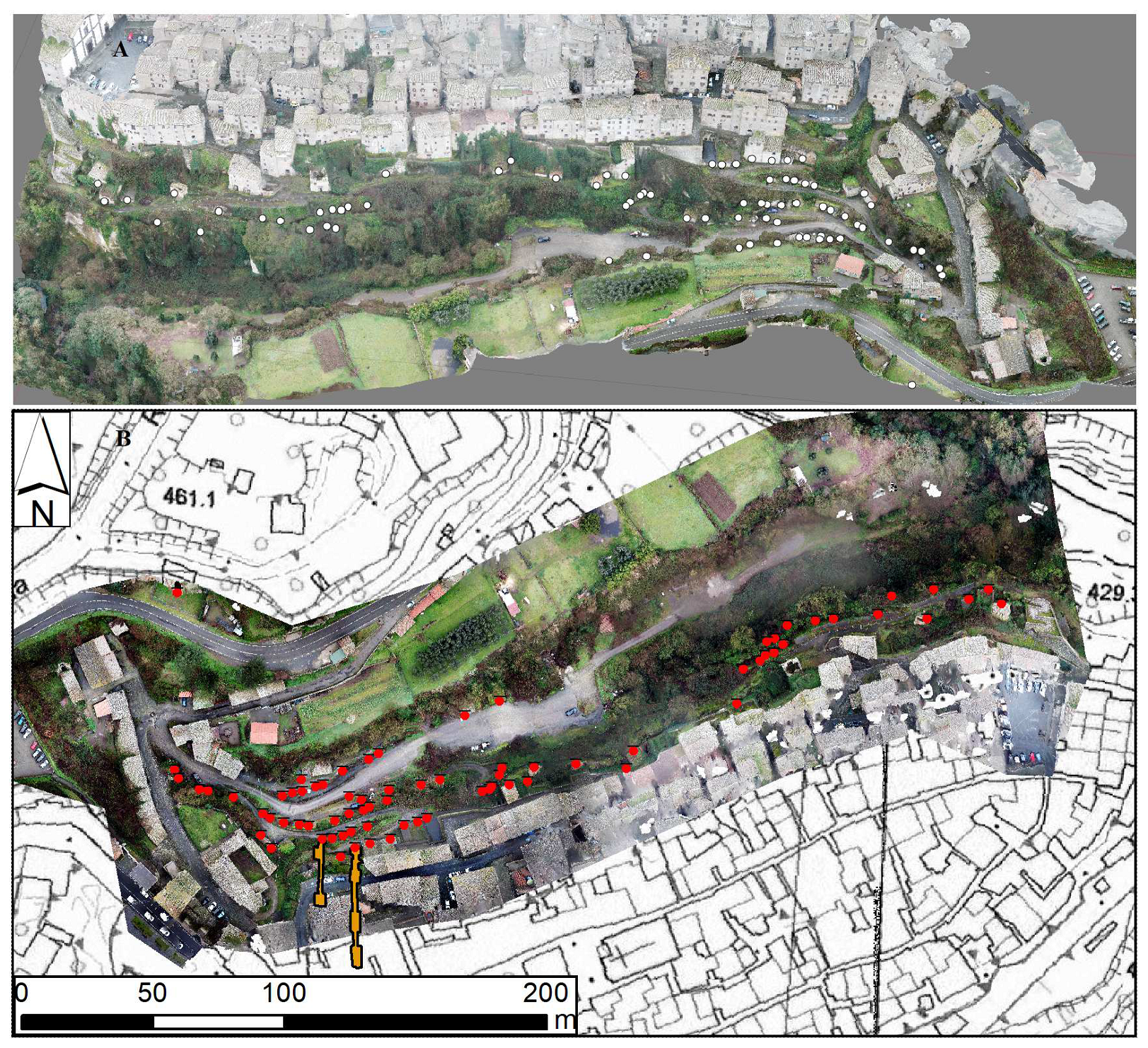
4.1. Photogrammetry
4.2. Lidar Surveys and Traditional Surveys

| Cavity | RMS (m) | Scale Factor |
|---|---|---|
| 1 | 0.035 | 0.972 |
| 2 | 0.029 | 0.986 |


4.3. Geomechanical Survey and Empirical Evaluation of Stability
| Number | Deep Direction (°) | Inclination (°) |
|---|---|---|
| 1 | 345 | 40 |
| 2 | 340 | 60 |
| 3 | 20 | 70 |
| 4 | 170 | 75 |
| 5 | 330 | 80 |
| 6 | 175 | 80 |
| 7 | 185 | 75 |
| Number | Deep Direction (°) | Inclination (°) |
|---|---|---|
| 1 | 340 | 65 |
| 2 | 170 | 85 |
| 3 | 355 | 70 |
| 4 | 95 | 80 |
| 5 | 355 | 80 |
| 7 | 185 | 75 |
| 8 | 170 | 65 |
| 9 | 170 | 70 |
| S | T | L | cosθ | CS | Sc |
|---|---|---|---|---|---|
| 2.3000 | 5.6500 | 3.7400 | 0.9850 | 1.3123 | 7.9271 |
| 3.5300 | 12.3600 | 4.3600 | 0.9850 | 1.2864 | 7.9271 |
| 1.2800 | 23.8100 | 12.8000 | 0.9850 | 0.4311 | 7.9271 |
| 4.3400 | 24.6300 | 5.1000 | 0.9850 | 1.1078 | 7.9271 |
| S | T | L | cosθ | CS | Sc |
|---|---|---|---|---|---|
| 4.0100 | 6.8500 | 8.5200 | 0.9850 | 1.8132 | 7.9271 |
| 3.8400 | 15.0400 | 4.8200 | 0.9850 | 1.0909 | 7.9271 |
| 1.9000 | 17.8600 | 11.2300 | 0.9850 | 0.5745 | 7.9271 |
| 4.0200 | 22.7800 | 7.5500 | 0.9850 | 0.9826 | 7.9271 |
| 1.8000 | 25.3200 | 5.0600 | 0.9850 | 0.4353 | 7.9271 |
| 3.8700 | 25.8400 | 8.5000 | 0.9850 | 0.9043 | 7.9271 |
| Q′ | A | B | C (Falls) | C (Sliding) | N (Falls) | N (Sliding) | S |
|---|---|---|---|---|---|---|---|
| 7.5 | 0.1 | 0.7 | 2.1 | 2.1 | 1.1025 | 1.1025 | 0.65 |
| 7.5 | 0.1 | 0.7 | 2.1 | 2.1 | 1.1025 | 1.1025 | 0.87 |
| 7.5 | 0.1 | 0.7 | 1.5 | 2.1 | 0.7875 | 1.1025 | 0.36 |
| 7.5 | 0.1 | 0.7 | 2.1 | 2.1 | 1.1025 | 1.1025 | 0.78 |
| Q′ | A | B | C (Falls) | C (Sliding) | N (Falls) | N (Sliding) | S |
|---|---|---|---|---|---|---|---|
| 7.5 | 0.1 | 0.65 | 1.5 | 2.1 | 0.73125 | 1.02375 | 1.04 |
| 7.5 | 0.1 | 0.65 | 1.5 | 2.1 | 0.73125 | 1.02375 | 0.88 |
| 7.5 | 0.1 | 0.65 | 2.1 | 2.1 | 1.02375 | 1.02375 | 0.51 |
| 7.5 | 0.1 | 0.65 | 1.5 | 2.1 | 0.73125 | 1.02375 | 0.82 |
| 7.5 | 0.1 | 0.65 | 2.1 | 2.1 | 1.02375 | 1.02375 | 0.49 |
| 7.5 | 0.1 | 0.65 | 1.5 | 2.1 | 0.73125 | 1.02375 | 0.75 |

5. Discussion
6. Conclusions
Author Contributions
Funding
Data Availability Statement
Acknowledgments
Conflicts of Interest
References
- Fairbridge. The Encyclopedia of Geomorphology; Ed. Reinhold: New York, NY, USA, 1968; 1295p. [Google Scholar]
- Nisio, S. The Sinkholes: Teminological Problmes, Genetic Mechanism, Classification. Mem. Descr. Carta Geol. It. 2008, 85, 17–32. [Google Scholar]
- Available online: https://www.isprambiente.gov.it/it/attivita/suolo-e-territorio/sinkholes-e-cavita-sotterranee/classificazione-dei-sinkholes (accessed on 26 March 2024).
- Ciotoli, G.; Di Loreto, E.; Finoia, M.G.; Liperi, L.; Meloni, F.; Nisio, S.; Sericola, A. Sinkhole susceptibility, Lazio Region, central Italy. J. Maps 2016, 12, 287–294. [Google Scholar] [CrossRef]
- Vennari, C.; Parise, M. A Chronological Database about Natural and Anthropogenic Sinkholes in Italy. Geosciences 2022, 12, 200. [Google Scholar] [CrossRef]
- Delle Rose, M.; Federico, A.; Parise, M. Sinkhole genesis and evolution in Apulia, and their interrelations with the anthropogenic environment. Nat. Hazards Earth Syst. Sci. 2004, 4, 747–775. [Google Scholar] [CrossRef]
- Parise, M.; De Pascalis, A.; De Pascalis, F.; Donno, G.; Inguscio, S. Cavita sotterranee a fini estrattivi, e loro connessione con fenomeni di sprofondamento e subsidenza in agro di Cutrofiano (Lecce). In Proceedings of the Spelaion 2006, Borgo Celano, Italy, 8–10 December 2008; pp. 55–69. [Google Scholar]
- Bonamini, M.; Di Maggio, C.; Lollino, P.; Madonia, G.; Parise, M.; Vattano, M. Sprofondamenti di origine antropica nell’area di Marsala (Sicilia occidentale) analizzati mediante rilievi in sito e analisi numerica dei processi di instabilità nelle cave sotterranee. Mem. Descr. Della Carta Geol. It. 2013, 93, 105–120. [Google Scholar]
- Tufano, R.; Guerriero, L.; Annibali Corona, M.; Bausilio, G.; Di Martire, D.; Nisio, S.; Calcaterra, D. Anthropogenic sinkholes of the city of Naples, Italy: An update. Nat. Hazards 2022, 112, 2577–2608. [Google Scholar] [CrossRef]
- Nisio, S.; Caramanna, G.; Ciotoli, G. Sinkholes in Italy: First results on the inventory and analysis. Geol. Soc. Lond. Spec. Publ. 2007, 279, 23–45. [Google Scholar] [CrossRef]
- Madonna, S.; Nisio, S.; Finocchiaro, G.; Gentili, F. Le cavità antropiche presenti nel sottosuolo di Bolsena. Mem. Descr. Carta Geol. d’It. 2020, 107, 383–396. [Google Scholar]
- Madonna, S.; Nisio, S.; Vessella, F. Primo contributo al censimento delle cavità sotterranee di Viterbo. Mem. Descr. Carta Geol. d’It. 2021, 108, 339–352. [Google Scholar]
- Oliveira, S.; Moura, D.; Boski, T.; Horta, J. Coastal paleokarst landforms: A morphometric approach via UAV for coastal management (Algarve, Portugal case study). Ocean Coast. Manag. 2019, 167, 245–261. [Google Scholar] [CrossRef]
- Pingel, T.J.; Saavedra, A.; Cobo, L. Deriving Land and Water Surface Elevations in the Northeastern Yucatán Peninsula Using PPK GPS and UAV-Based Structure from Motion. Pap. Appl. Geogr. 2021, 7, 294–315. [Google Scholar] [CrossRef]
- Puzzilli, L.; Ruscito, V.; Madonna, S.; Gentili, F.; Ruggiero, L.; Ciotoli, G.; Nisio, S. Natural sinkhole monitoring and characterization: The case of Latera sinkhole (Central Italy). Geosciences 2024, 14, 18. [Google Scholar] [CrossRef]
- Monsalve, A.; Yager, E.M.; Tonina, D. Evaluating Apple iPhone LiDAR measurements of topography and roughness elements in coarse bedded streams. J. Ecohydraulics 2023. early access. [Google Scholar] [CrossRef]
- King, F.; Kelly, R.; Fletcher, C.G. New opportunities for low-cost LiDAR-derived snow depth estimates from a consumer drone-mounted smartphone. Cold Reg. Sci. Technol. 2023, 207, 103757. [Google Scholar] [CrossRef]
- Díaz-Vilariño, L.; Tran, H.; Frías, E.; Balado, J.; Khoshelham, K. 3D Mapping of Indoor And Outdoor Environments Using Apple Smart Devices. ISPRS-Int. Arch. Photogramm. Remote Sens. Spat. Inf. Sci. 2021, 43-B4, 303–308. [Google Scholar] [CrossRef]
- Teo, T.A.; Yang, C.C. Evaluating the accuracy and quality of an iPad Pro’s built-in lidar for 3D indoor mapping. Dev. Build Environ. 2023, 14, 100169. [Google Scholar] [CrossRef]
- Rutkowski, W.; Lipecki, T. Use of the iPhone 13 Pro LiDAR Scanner for Inspection and Measurement in the Mineshaft Sinking Process. Remote Sens. 2023, 15, 5089. [Google Scholar] [CrossRef]
- Silva, O.L.; Bezerra, F.H.R.; Maia, R.P.; Cazarin, C.L. Karst landforms revealed at various scales using LiDAR and UAV in semi-arid Brazil: Consideration on karstification processes and methodological constraints. Geomorphology 2017, 295, 611–630. [Google Scholar] [CrossRef]
- I.S.R.M. (International Society for Rock Mechanics). Suggested methods for the quantitative description of discontinuities in rock masses. Int. J. Rock Mech. Min. Sci. Geomech. Abstr. 1978, 15, 319–368. [Google Scholar]
- I.S.R.M. (International Society for Rock Mechanics). Basic geotechnical description of rock masses. Int. J. Rock Mech. Min. Sci. Geom. Abstr. 1981, 18, 85–110. [Google Scholar]
- I.S.R.M. (International Society for Rock Mechanics). Rock Characterization, Testing and Monitoring; Brown, E.T., Ed.; Pergamon Press: Oxford, UK, 1981; p. 211. [Google Scholar]
- Harp, E.L.; Noble, M.A. An Engineering Rock Classification to Evaluate Seismic Rock-Fall Susceptibility and its Application to the Wasatch Front. Environ. Eng. Geosci. 1993, 30, 293–319. [Google Scholar] [CrossRef]
- Carter, T.G. A new approach to surfacecrown pillar design. In Proceedings of the 16th Canadian Rock Mechanics Symposium, Sudbury, ON, Canada; 1992; pp. 75–83. [Google Scholar]
- Potvin, Y.; Milne, D. Empirical cable bolt support design. In Rock Support in Mining and Underground Construction. In Proceedings of the 16th Canadian Rock Mechanics Symposium. Sudbury, ON, Canada, 1992; Kaiser, P.K., McCreath, D.R., Eds.; Balkema: Rotterdam, The Netherlands, 1992. [Google Scholar]
- Zhao, X.; Li, H.; Zhang, S.; Yang, X. Stability Analyses and Cable Bolt Support Design for A Deep Large-Span Stope at the Hongtoushan Mine, China. Sustainability 2019, 11, 6134. [Google Scholar] [CrossRef]
- Sapia, V.; Materni, V.; Florindo, F.; Marchetti, M.; Gasparini, A.; Voltattorni, N.; Civico, R.; Giannattasio, F.; Miconi, L.; Marabottini, M.F.; et al. Imaging multiparametrico di tombe a camera etrusche: Caso di studio Grotte Di Castro (Italia). Appl. Sci. 2021, 11, 7875. [Google Scholar] [CrossRef]
- Ciotoli, G.; Finoia, M.G.; Liperi, L.; Meloni, F.; Nisio, S.; Tonelli, V.; Zizzari, P. Sinkhole susceptibility map of the Lazio Region, central Italy. J. Maps 2015, 12, 287–294. [Google Scholar] [CrossRef]
- Washington, H.S. The Roman Comagmatic Rgion; Carnegie Institute Washington: Washington, DC, USA, 1906; Volume 36, pp. 1–220. [Google Scholar]
- Locardi, E.; Lombardi, G.; Funiciello, R.; Parotto, M. The main volcanic groups of the Latium (Italy): Relations between structural evolution and petrogenesis. Geol. Romana 1976, 16, 279–300. [Google Scholar]
- Sparks, R.S.J. Stratigraphie et géologie des ignimbrites du volcan Vulsini, Italie centrale. Geol. Rundsch. 1975, 64, 497–523. [Google Scholar] [CrossRef]
- Peccerillo, A. Cenozoic Volcanism in the Tyrrhenian Sea Region; Springer: Berlin/Heidelberg, Germany, 2017. [Google Scholar] [CrossRef]
- Nappi, G.; Renzulli, A.; Santi, P. An evolutionary model for the Paleo-Bolsena and Bolsena volcanic complexes: A structural and petrographic study. Per Miner. 1987, 56, 241–267. [Google Scholar]
- Nappi, G.; Renzulli, A.; Santi, P. Evidence of incremental growth in the Vulsinian calderas (central Italy), in Verma-Surendra, P., ed., Calderas: Genesis, Structure and Unrest. J. Volcanol. Geotherm. Res. 1991, 47, 13–31. [Google Scholar] [CrossRef]
- Vezzoli, L.; Conticelli, S.; Innocenti, F.; Landi, P.; Manetti, P.; Palladino, D.M.; Trigila, R. Stratigraphy of the Latera volcanic complex: Proposals for a new nomenclature. Period. Mineral. 1987, 56, 89–110. [Google Scholar]
- Metzelin, S.; Vezzoli, L. Santa Contributi alla geologia del Vulcano di Latera (Monti Vulsini, Toscana meridionale, Lazio settentrionale). Mem. Soc. Geol. It. 1983, 25, 247–273. [Google Scholar]
- Turbeville, B.N. Tephra fountaining, rheomorphism, and spatter flow during emplacement of the Pitigliano Tuffs, Latera caldera, Italy. J. Volcanol. Geotherm. Res. 1992, 53, 309–327. [Google Scholar] [CrossRef]
- Palladino, D.M.; Simei, S.; Sottili, G.; Trigila, R. Integrated approach for the reconstruction of stratigraphy and geology of Quaternary volcanic terrains: An application to the Vulsini Volcanoes (central Italy). In Stratigraphy and Geology in Volcanic Areas; Groppelli, G., Viereck-goette, L., Eds.; Geological Society of America: Boulder, CO, USA, 2010; Volume 464, pp. 66–84. [Google Scholar] [CrossRef]
- Valerio, A.; Danilo, P.; Raffaello, C.; Russo, P.; Simei, S. Caldera structure, amount of collapse, and erupted volumes: The case of Bolsena caldera, Italy. Geol. Soc. Am. Bull. 2012, 124, 1562–1576. [Google Scholar] [CrossRef]
- Bizzarri, R.; Ambrosetti, P.; Argenti, P.; Gatta, G.; Baldanza, A. L’affioramento del Caio (Lago di Corbara, Orvieto, Italia Centrale) nell’ambito dell’evoluzione paleogeografica Plio-Pelistocenica della Valle del Tevere: Evidenze sedimentologiche e stratigrafiche. Il Quat. 2003, 16, 241–255. [Google Scholar]
- Bizzarri, R.; Baldanza, A.; Petrelli, M.; Famiani, F.; Peccerillo, A. Early Pleistocene distal pyroclastic-fallout material in continental and marine deposits of Western Umbria (Italy): Chemical composition, provenance and correlation potential. Il Quat. 2010, 23, 245–250. [Google Scholar]
- Available online: https://idrogeo.isprambiente.it/app/pir?@=41.55172525858242,12.573501484000001,2 (accessed on 12 April 2024).
- Available online: https://www.isprambiente.gov.it/it/attivita/suolo-e-territorio/cartografia/carte-geologiche-e-geotematiche/carta-geologica-alla-scala-1-a-100000 (accessed on 10 April 2024).
- Palladino, D.M.; Pettini, M. Source- vs. topographic-forcing in pyroclastic currents: The case of the Orvieto-Bagnoregio Ignimbrite, Vulsini, central Italy. Period. Mineral. 2020, 89, 217–229. [Google Scholar]
- Cloud Compare (version 2.1) [GPL Software]. 2024. Available online: http://www.cloudcompare.org/ (accessed on 15 February 2024).
- Barton, N. Rock mass classification, tunnel reinforcement selection using the Q-system. In Rock Classification Systems for Engineering Purposes; ASTM International: West Conshohocken, PA, USA, 1987. [Google Scholar]
- Barton, N.; Lien, R.; Lunde, J. Engineering classification of rock masses for the design of tunnel support. Rock Mech. 1974, 6, 188–236. [Google Scholar] [CrossRef]
- Brown, E.T.; Bray, J.W.; Ladanyi, B.; Hoek, E. Characteristic line calculations for rock tunnels. J. Geotech. Engng Div. ASCE 1983, 109, 15–39. [Google Scholar] [CrossRef]
- Carter, T.G. Guidelines for use of the Scaled Span Method for Surface Crown Pillar Stability Assessment; Ontario Ministry of Northern Development and Mines: Toronto, ON, Canada, 2014; pp. 1–34. [Google Scholar]
- Hoek, E.; Brown, E.T. Empirical strength criterion for rock masses. J. Geotech. Eng. Div. 1980, 106, 1013–1035. [Google Scholar] [CrossRef]
- Hoek, E.; Brown, E.T. Underground Excavations in Rock; Institute of Mining and Metallurgy: London, UK, 1980. [Google Scholar]
- Hoek, E.; Brown, E.T. Practical estimates of rock mass strength. Int. J. Rock Mech. Min. Sci. 1997, 34, 1165–1186. [Google Scholar] [CrossRef]
- Luetzenburg, G.; Kroon, A.; Bjørk, A.A. Evaluation of the Apple iPhone 12 Pro LiDAR for an Application in Geosciences. Sci. Rep. 2021, 11, 22221. [Google Scholar] [CrossRef]
- Tavani, A.; Billi, A.; Corradetti, A.; Mercuri, M.; Bosman, A.; Cuffaro, M.; Seers, T.; Carminati, E. Smartphone assisted fieldwork: Towards the digital transition of geoscience fieldwork using LiDAR-equipped iPhones. Earth-Sci. Rev. 2022, 227, 103969. [Google Scholar] [CrossRef]
| Q″ | Susceptibility to Collapse for Seismic Event of Magnitude > 5 |
|---|---|
| <0.1 | Very high |
| 0.1–1 | High |
| 1–9.99 | Medium |
| >10 | Low |
| GPS | Error (m) | Lead Time (Minutes) |
|---|---|---|
| GNSS Station | 0.037 (on GCP) 0.043 (on CP) | 68 |
| Mavic Pro GPS | 1.7 | 21 |
| Method | Number of Entrances | Lead Time (Minutes) |
|---|---|---|
| UAV Model | 76 | 64 |
| Reconnaissance | 58 | 145 |
| Cavity | Surface m2 (iPhone) | Perimeter m (iPhone) | Surface m2 (Traditional) | Perimeter m (Traditional) |
|---|---|---|---|---|
| 1 | 63.7 | 69.44 | 61.88 | 68.32 |
| 2 | 133.29 | 111.52 | 129.81 | 110.67 |
| Cavity | Q′ | Classification Class |
|---|---|---|
| 1 | 7.5 | V (mediocre) |
| 2 | 7.5 | V (mediocre) |
Disclaimer/Publisher’s Note: The statements, opinions and data contained in all publications are solely those of the individual author(s) and contributor(s) and not of MDPI and/or the editor(s). MDPI and/or the editor(s) disclaim responsibility for any injury to people or property resulting from any ideas, methods, instructions or products referred to in the content. |
© 2024 by the authors. Licensee MDPI, Basel, Switzerland. This article is an open access article distributed under the terms and conditions of the Creative Commons Attribution (CC BY) license (https://creativecommons.org/licenses/by/4.0/).
Share and Cite
Gentili, F.; Madonna, S. Photogrammetry from UAV and Low-Cost Lidar for Sinkhole Hazard Mitigation in Urban Areas: Applications and Evaluations. Geographies 2024, 4, 343-362. https://doi.org/10.3390/geographies4020020
Gentili F, Madonna S. Photogrammetry from UAV and Low-Cost Lidar for Sinkhole Hazard Mitigation in Urban Areas: Applications and Evaluations. Geographies. 2024; 4(2):343-362. https://doi.org/10.3390/geographies4020020
Chicago/Turabian StyleGentili, Francesco, and Sergio Madonna. 2024. "Photogrammetry from UAV and Low-Cost Lidar for Sinkhole Hazard Mitigation in Urban Areas: Applications and Evaluations" Geographies 4, no. 2: 343-362. https://doi.org/10.3390/geographies4020020