Article

Vegetation Structure and Distribution Across Scales in a Large Metropolitan Area: Case Study of Austin MSA, Texas, USA

1
Department of Geography and Environmental Studies, Texas State University, San Marcos, TX 78666, USA
2
School of Plant and Environmental Sciences, Virginia Tech, Blacksburg, VA 24061, USA
*
Author to whom correspondence should be addressed.
Geographies 2025, 5(1), 11; https://doi.org/10.3390/geographies5010011
Submission received: 23 January 2025 / Revised: 24 February 2025 / Accepted: 1 March 2025 / Published: 3 March 2025

Abstract

:
The spatial distribution of vegetation across metropolitan areas is important for wildlife habitat, air quality, heat mitigation, recreation, and other ecosystem services. This study investigated relationships between vegetation patterns and parcel characteristics at multiple scales of the Austin Metropolitan Statistical Area (MSA), a rapidly growing region in central Texas characterized by diverse biophysical and socioeconomic landscapes. We used LiDAR data to map vegetation types and distributions across a 6000 km2 study area. Principal component analysis (PCA) and regression models were employed to explore tree, shrub, and grass cover across parcels, cities, and the MSA, considering home value, age, size, and distance to the city center. At the MSA scale, tree and shrub cover were higher in the Edwards Plateau than in the Blackland Prairie ecoregion. Tree cover increased with parcel size and home value, especially in suburban areas. Older parcels had more mature trees, though less so in the grass-dominated Blackland Prairie. Shrub cover was higher on larger parcels in the Edwards Plateau, while the Blackland Prairie showed the opposite trend. PCA explained 60% of the variance, highlighting links between vegetation and urban development. Our findings reveal how biophysical and socioeconomic factors interact to shape vegetation, offering considerations for land use, housing, and green infrastructure planning.

Graphical Abstract

1. Introduction

Human activity alters land cover at all geographic scales [1,2,3]. Urbanization, in particular, can result in the complete removal of large areas of existing vegetation [4,5] and the creation of new green spaces to meet social demands [6,7]. Urban landscapes can therefore be dynamic, with altered vegetation patterns [6,8]. These altered ecosystems affect the supply of ecosystem services, including habitat, water quality, air quality, heat mitigation, and recreation [8,9,10,11]. Hence, accurate quantification of the spatial distribution of urban greenspace has brought increasing attention from geographers, ecologists, conservation scientists, urban planners, and policymakers [12,13]. The focus of existing research has predominantly been on the accessibility of greenspaces, sidelining the need for a thorough geographical assessment [14,15]. The vegetation at the neighborhood and parcel scales tends to be overshadowed by broader city- or regional-scale analyses, leading to a lack of detailed understanding in these small yet critical units [16]. Despite significant progress in determining the spatial distribution of tree canopy and total vegetation cover at city scales, cross-city and multi-scaled examinations of vegetation patterns are lacking but needed to meet climate adaptation and planning goals [16].
In cities, residential areas and their private greenspaces can account for a major portion of urban vegetation and habitat [17,18,19]. Bird diversity, as just one indicator, has been found to be higher in residential landscapes comprising diverse and dense yard vegetation [20,21]. Yards connected to natural forests and large landscape corridors can also influence animal movements and extents [22]. These findings suggest the importance of private vegetation cover for urban habitats; however, there is very little information on three-dimensional spatial patterns of vegetation at the parcel scale across the landscape [23,24]. Vegetation structure is the configuration and connectivity of plants in the landscape, influencing how urbanization is linked to ecosystem services [25]. For example, the spatial variability of woody vegetation across urban landscapes can affect many organisms [26,27,28,29,30]. Early studies focused on the areal coverage of vegetation, but the structure of vegetation is more meaningful.
Vegetation structure and patterns are affected by biophysical as well as numerous built, social, and economic factors [31,32]. Urban development is known to homogenize native ecosystems, making urban ecosystems more similar across ecoregions than the native ecosystem attributes [33]. However, there is still substantial variation in vegetation cover among cities, which is better related to ecoregions than political boundaries at the national scale [34]. Likewise, the degree of heterogeneity among individual cities within an urban amalgamation and the factors that might be influencing vegetation structure within those cities are still unknown. A metropolitan statistical area (MSA) will often have one large city and multiple smaller municipalities within its boundaries. While it might be expected that these smaller units will have similar vegetation patterns as the large central city, that has yet to be examined. Alternatively, factors such as population size, age of development, employment patterns, historical land use, land rents, and ecoregion boundaries may cause smaller cities and towns within the region to have very different vegetation distributions compared to the central city [31,35].
At individual city scales, the negative correlation between impervious surface area—a common proxy for urban development—and vegetation has been well documented [36,37,38]. This correlation results in city centers often having less vegetation cover than fringes of the city. Within a city, studies have found that social factors like wealth and practices like redlining can result in patchy distributions where some neighborhoods have greater tree cover and green space [31,39]. Urban design and planning choices like parcel size and characteristics have received little attention as factors affecting vegetation cover.
Light detection and ranging (LiDAR) technology has now made it possible to map and explore three-dimensional (3D) urban vegetation at sub-meter and, therefore, sub-parcel scales. There are two main drawbacks in vegetation height detection from LiDAR: (i) tree height underestimation and (ii) the occurrence of visible data pits. To address these two problems, canopy height models (CHMs) from LiDAR point clouds can use a selecting and sorting mechanism followed by spatial interpolation [40]. In addition, vegetation mapping can be improved by fusing multi-sensor data with the LiDAR point cloud, as the spectral information is missing for LiDAR data [41]. Hartfield et al. [42] found that the classification accuracy of multi-spectral images along with the Normalized Difference Vegetation Index (NDVI) can substantially improve the accuracy; adding the LiDAR-derived digital surface model (DSM) can further boost the accuracy since the DSM data avoids mixing herbaceous with tree/shrub classes. MacFaden et al. [43] combined very-high-resolution multispectral orthoimage data and airborne LiDAR data for urban tree canopy mapping. Their findings demonstrated that the use of the NDVI and the DSM are vital to extracting tree features adjacent to buildings. Because of the success of these case studies, multi-sensor data fusion offers a promising solution for diverse vegetation cover.
Using advanced LiDAR technology and methods, our study assessed vegetation structure and distributions of the Austin MSA (Texas, USA), one of the fastest-growing metropolitan areas in the nation. The Austin MSA is comprised of one large central city as well as multiple suburbs and towns. The MSA is also intersected by two major ecoregions, which offered an opportunity to study how urbanization interacts with physical geography to affect vegetation patterns. We investigated the three-dimensional (3D) structure and distribution of vegetation in single-family residential parcels across the entire Austin MSA. Our objectives were to (1) compare the urban vegetation patterns of two distinct ecoregions of the MSA, (2) determine how parcel scale attributes (size, distance to city center, home value, and age) account for variation in the city- and MSA-scale vegetation patterns, and (3) compare vegetation patterns for each of the 10 municipalities. To achieve these objectives, we assessed vegetation structures at the parcel, city, and MSA scales using USGS 3DEP LiDAR to create a CHM and extract vegetation metrics, while identifying parcel characteristics.

2. Materials and Methods
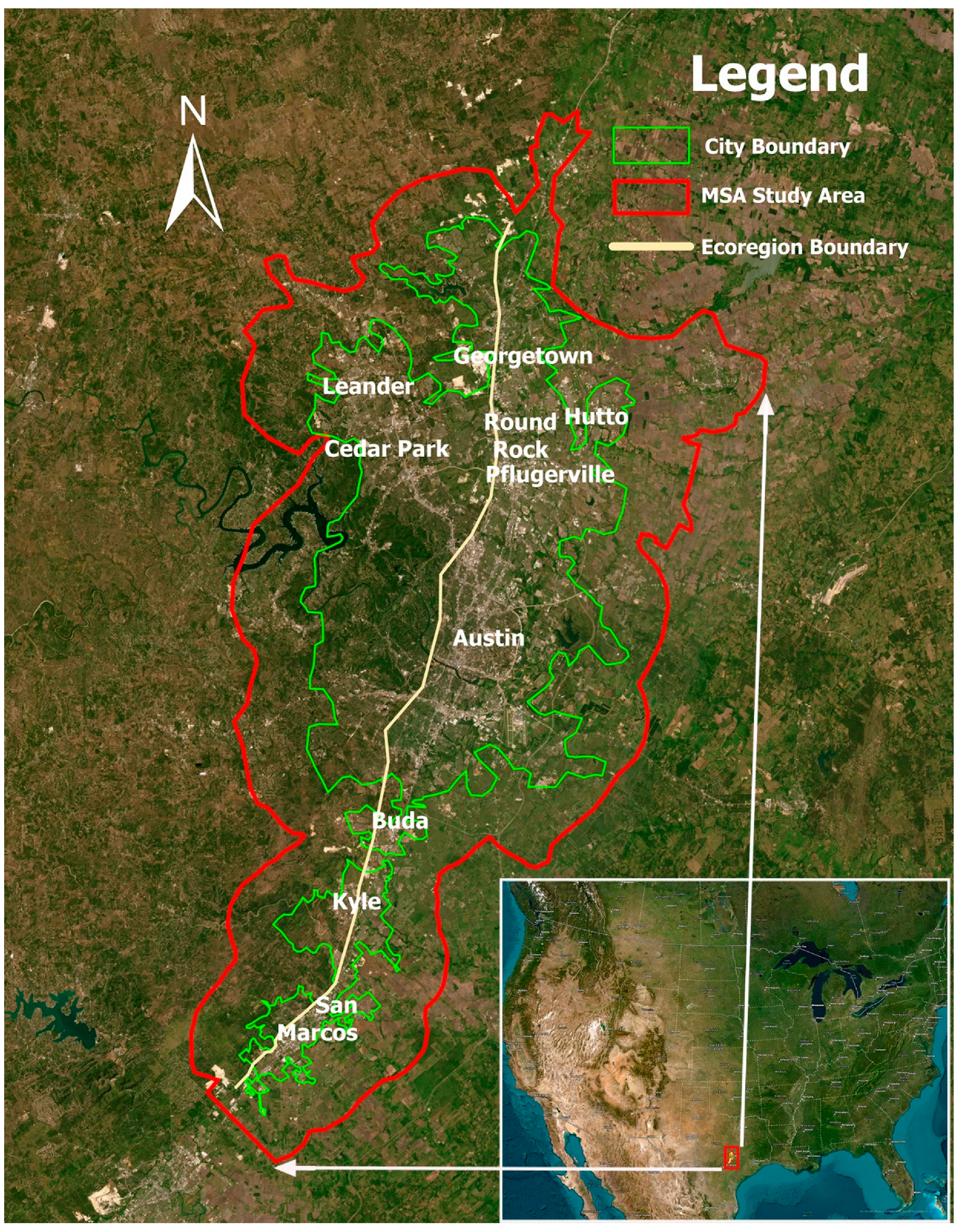
2.1. Study Area

We selected ten cities (population > 20,000) and their extended extra-territorial jurisdiction (ETJ) in the Austin MSA to analyze vegetation distributions (Figure 1). The ETJ in Texas is a designated buffer area around the outside of the city limits, which defines potential growth and future service boundaries. It can range from 0.8 km for cities with less than 5000 people to 8 km for cities with more than 100,000 people. The study area encompassing the Austin MSA covered approximately 6000 km2. The Austin MSA has been one of the fastest-growing metropolitan areas since 2000 and has seen an 88% increase in population between 2000 and 2021 [44].
The vegetation of the Austin MSA is influenced by its semi-arid climate, with a mean annual precipitation of 90 cm [45]. Our Austin MSA study area is divided into two ecoregions (Figure 1): Edwards Plateau (to the west) and Blackland Prairie (to the east) [46]. The Edwards Plateau (EP) ecoregion has more topographical variation and a limestone-based geology, with a variety of grasses and shrubs adapted to its rocky soils [47]. The Blackland Prairie (BP), on the other hand, is distinguished by its productive soils and agriculture; however, urban development has replaced many agricultural lands within the ETJ [48].

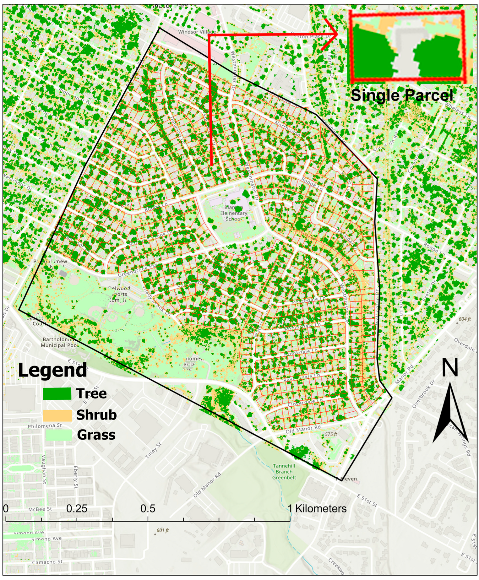
2.2. LiDAR Vegetation Mapping

The U.S. Geological Survey (USGS) 3D Elevation Program (3DEP) LiDAR provides wall-to-wall coverage for many states in the USA [49]. We followed a canopy height mapping workflow with 3DEP LiDAR across the Austin MSA [50]. LiDAR datasets during 2015–2017 with 1 m spatial resolutions were available for our study area. The digital elevation model (DEM) and NDVI from NAIP imagery were used as input data in this study. We converted raw LiDAR point clouds stored in laz format to las format using the ArcGIS Pro 2.6 Convert las tool. Subsequently, the conversion of the las file into a raster DSM was accomplished through the utilization of the las to raster dataset tool. To ensure spatial consistency, all rasters (DSM and DEM) were projected to a common coordinate system (NAD 1983 UTM Zone 14N) and resampled to a uniform 1 m resolution. We used the data filtering process in ArcGIS Pro 2.6 to remove the noise and selected the first return DSM by using the all-returns filter on the LAS dataset toolbar. We applied the mosaicking of all the datasets for our study area using the ERDAS Imagine 16.6 Mosaic Pro tool. Finally, to derive the canopy height, we subtracted the DSM from the DEM.
The vertical resolution of the LiDAR-derived DSM and DEM was consistent with the original LiDAR point cloud, which had an average point spacing of 1 m and a vertical accuracy of ±0.196 m (RMSE) in non-vegetation areas and ±0.3 m (RMSE) in vegetation areas (source: image metadata). To ensure alignment, we checked the DSM and DEM for both vertical and horizontal consistency, minimizing potential mismatches. While vegetation height classification was based on the LiDAR-derived CHM, NAIP imagery was used primarily for vegetation mapping and visualization, rather than for height-based analyses.
We masked buildings and water bodies in the analysis using datasets for building footprints and water bodies, which were collected from the GIS open data portals of each city’s website [50]. We included only wide roads (A1–A3; at least two lanes and >45 mph speed limit) in the masking process because removing smaller roads risked eliminating roadside trees. We excluded non-vegetation elements from the analysis by utilizing the NDVI and vegetation land cover generated from the 2018 NAIP imagery (0.6 m resolution). In this process, we incorporated the vegetation classes from the NAIP land-cover map. Land-cover maps have the limitation of confusing some vegetation cover as shadow, which we addressed by using a threshold value for the NDVI dataset. From this refined dataset, we then extracted the areas designated as vegetation for subsequent analysis by the CHM. Following the acquisition of the vegetation height map, we applied a manual procedure to eliminate outliers, including utility poles and transmission lines.
We validated the accuracy of LiDAR-based canopy heights by conducting a comparative analysis with height metrics extracted from the Forest Inventory and Analysis (FIA) dataset for 2017 and 2018, focusing exclusively on the Austin area due to the availability of FIA data and the timing of image acquisition [50]. For this validation, we used points greater than 2 m above ground to calculate average LiDAR heights and compared these with tree heights derived from FIA data. The evaluation centered on analyzing the discrepancies between LiDAR-derived and inventory-derived heights. We meticulously assessed these differences considering various factors, such as LiDAR point density, recorded inventory height, the year of LiDAR data and inventory data collection, and the time interval between the acquisition of LiDAR and inventory data.

2.3. Vegetation Classification Based on Height

To analyze vegetation distributions across scale in urban areas, we first defined tree canopy cover and separated it from shrubs and grassland. Trees are classified in multiple ways [51,52], but for the purpose of this study, we defined them as vegetation coverage above a certain height, as derived from the CHM. Brokaw [53] used a threshold height of 2 m to define the canopy shape. Ucar et al. [54] separated LiDAR point clouds in two classes: (1) points greater than 0.2 m and less than 6 m as shrubs, and (2) points greater than 6 m as trees. Weinstein et al. [55] used a 3 m threshold value to define trees in their studies on NEON sites. Based on the literature and taking into account the vegetation characteristics of our semi-arid study area, we selected the following height ranges for vegetation cover: grass (<0.2 m), shrub (0.2–3.0 m), and tree (>3.0 m). Along with measurements of grass, shrub, and tree cover, we incorporated metrics such as median tree height and maximum tree height as part of the vegetation structure analysis.

2.4. Selection of Predictor/Independent Variables and Overlay Analyses

The type and distribution of vegetation in urban neighborhoods and residential parcels are influenced by a variety of factors, including local climate, soil properties, zoning regulations, ecological attributes, socioeconomic conditions, and cultural elements [56,57,58,59]. To assess socioeconomic factors at the parcel scale, we focused on four parcel characteristics that have likely impacted vegetation attributes: parcel size, distance to city center, home age, and home value (Table 1).
We collected the age and market value of homes for each single-family residential parcel from Texas County Appraisal District (CAD) datasets obtained from each county’s government website [50]. A considerable proportion of parcels displayed missing home construction dates. We addressed this issue by manually collecting the missing home age and home value data from Zillow, a well-known online platform for real estate information. Despite manual collection efforts, about 10% of the parcels in two counties still lacked recorded home age data: Hays County (cities of San Marcos, Kyle, and Buda) and Williamson County (cities of Round Rock and Georgetown). The distance of a home/parcel from the city center could have multiple influences on its vegetation characteristics related to historical legacies in development patterns, land values, and vegetation age [60,61]. To determine whether these patterns and relationships exist within the Austin MSA, we calculated the distance of each parcel and neighborhood from the city’s central administrative location (e.g., county/city courthouse).
To compare vegetation metrics and parcel characteristics (Figure 2), we utilized the Extract by Mask and Zonal Statistics tools from the ArcGIS Pro Spatial Analyst Toolset. The Extract by Mask tool was used to clip the CHM raster to the study parcel, ensuring only relevant vegetation data were considered. The Zonal Statistics tool was then applied to calculate the pixel count and then the percentage share of each vegetation type within individual parcels (Figure 2). This process allowed us to quantify and analyze the relationship between parcel vegetation attributes and other parcel characteristics, such as size, age, and value.

2.5. Statistical Analyses

We analyzed vegetation metrics in relation to parcel characteristics (parcel size, home value, home age, distance to the city center) at the parcel scale using multiple linear regression. Normality tests were performed at the parcel level, revealing that while home value and home age were approximately normally distributed, parcel size and distance to the city center required logarithmic transformations to address skewness. Tree cover exhibited a zero-inflated distribution, with many parcels having no tree cover. Accordingly, we applied a Tobit regression model, which accounts for censored dependent variables [62]. We employed stepwise regression at the parcel level to understand the relative impact of variables. This method iteratively added variables based on their contributions to the model, assessed through changes in Akaike information criterion (AIC) values and increases in R2. Stepwise regression allowed us to identify the most informative predictors while balancing model complexity, ensuring a more robust and interpretable final model. For the above statistical analyses, we used R programming language.
To further understand the relationship between vegetation and parcel characteristics, we conducted a principal component analysis (PCA). First, we addressed missing values and standardized the dataset to address the differences in variable scales. The standardization process was achieved by transforming the data to have a mean of zero and unit variance using the StandardScaler function from the scikit-learn library in Python 3.7. This transformation standardized the vegetation and parcel characteristics variables by subtracting the mean and scaling to unit variance to ensure comparability across different scales. For the PCA, we selected two principal components (PC1 and PC2), as they captured the most variance in the data. After fitting the PCA model, we examined the proportion of variance explained by each principal component. We extracted the principal components, i.e., transformed data that represent the observations (e.g., cities or parcels) projected onto the PC1 and PC2 axes. We also calculated the loadings, which indicate the contributions of the original variables to each principal component. These loadings were essential for interpreting how the variables influenced the principal components. For visualization, we constructed a PCA biplot, which displays the principal components of each observation as a scatter plot, where city–ecoregion combinations represent sample points. The arrows in a PCA biplot show how much each original variable influences the principal components, indicating both the strength and the direction of their contribution. Finally, the axes were labeled with the percentage of variance explained by PC1 and PC2 to interpret how well these components summarized the original dataset.

3. Results

3.1. Parcel Characteristics

The Austin MSA study area had a total of 586,678 parcels, with 391,601 identified as single-family residential parcels, in the 2020 CAD datasets (Table 2). Out of these 391,601 parcels, 40% of the parcels were in the Edwards Plateau (EP) ecoregion and the other 60% were in the Blackland Prairie (BP) ecoregion. The median area for single-family residential parcels ranged from 0.07 to 0.12 ha across the ten cities. In general, cities located north of Austin, such as Cedar Park, Georgetown, Leander, and Round Rock, exhibited larger median parcel sizes (Table 2). In these northern cities, the differences in parcel sizes between the two ecoregions were minimal. Cities south of Austin, including Kyle and San Marcos, showed notably smaller median parcel sizes. In some cities (Austin, Georgetown, San Marcos), parcels within the EP had significantly larger median sizes compared to those in the BP (Table 2).
Home values across the study area were highest in Austin, followed by its northern suburbs of Georgetown, Round Rock, Cedar Park, and Leander (Table 2). In contrast, the southern cities of San Marcos, Buda, and Kyle had the lowest median home values. Home values in the EP ecoregion were significantly higher across all MSA cities compared to the BP ecoregion. Home age also displayed a north–south pattern (Table 2). Northern cities generally had newer homes, with median ages ranging from 10 to 20 years. In contrast, cities like Austin, San Marcos, and Buda had older housing stock, with median ages of between 29 and 49 years. Georgetown, which had the largest median parcel size, also exhibited a relatively new housing stock, with a median age of 15 years. Austin BP stood out with a median home age of 49 years, the oldest among the cities. Between ecoregions, the EP had more newer homes compared to the BP.
Distance to city center revealed two patterns (Table 2). First, Austin and Buda exhibited greater distances due to their large areas and extensive suburban developments. Second, parcels in the EP were generally farther from the city center compared to those in the BP. A comparison among the ten cities revealed that cities farther from downtown Austin exhibited larger parcels with newer and less expensive homes, while cities closer to downtown Austin had smaller parcels and older, more expensive homes, reflecting the denser, more developed urban environment.

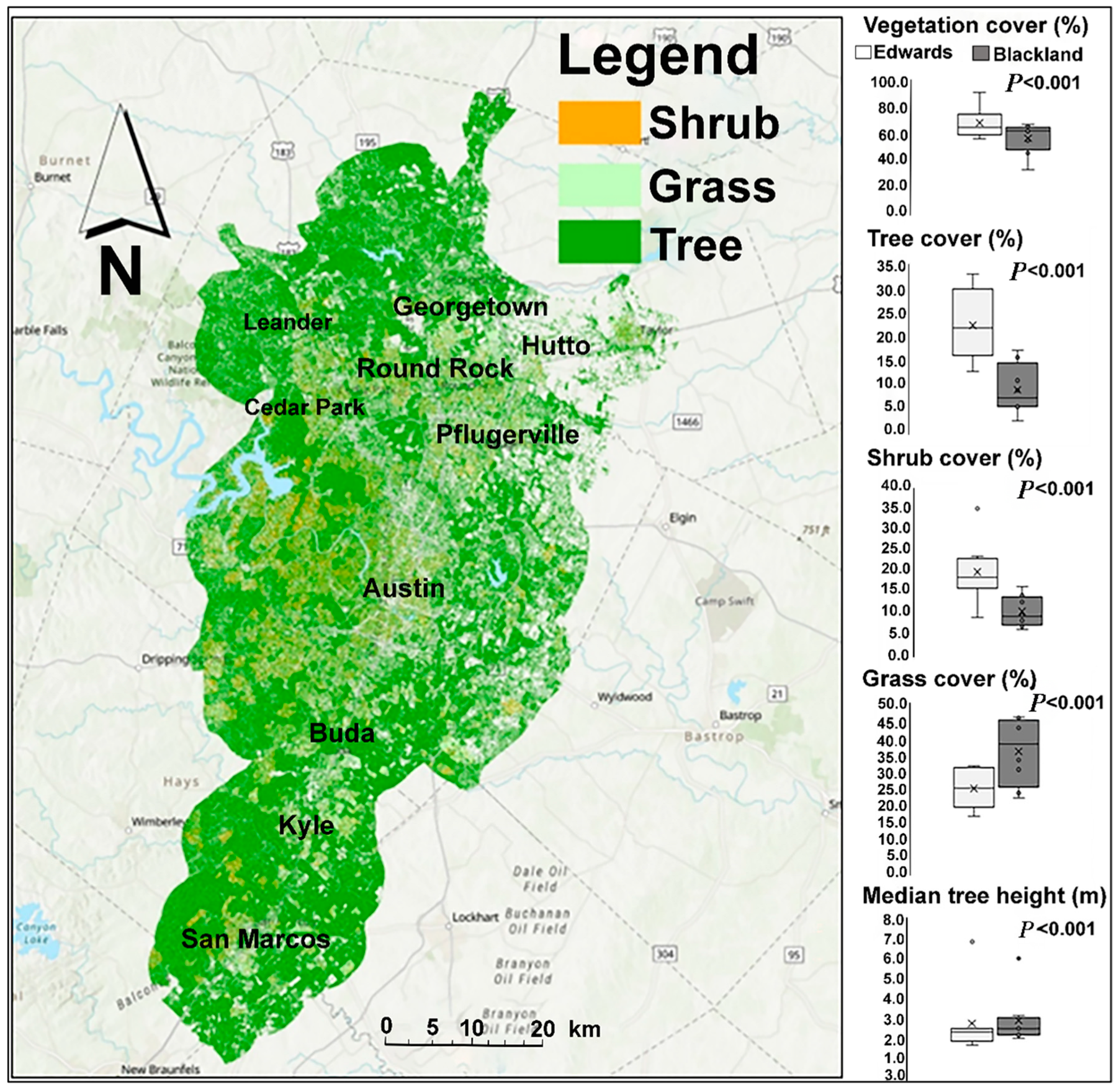
3.2. Vegetation Characteristics

The canopy height model (CHM) metrics showed a moderate to strong correlation with the FIA inventory heights. The maximum height from the inventory and the maximum CHM height had a correlation of 0.90. The correlation between the mean CHM height and the maximum inventory height was 0.73. The mean CHM height and the mean FIA inventory height correlated at 0.64. These findings indicated that the CHM model demonstrated a relatively high level of accuracy with in situ field measurements.

3.3. Vegetation and Parcel Comparisons at MSA Scale

The vegetation cover across the Austin MSA revealed distinct patterns influenced by ecoregion characteristics (Figure 3). The hilly, higher-elevation EP ecoregion had higher total vegetation cover, along with higher tree and shrub cover. In contrast, the flat BP ecoregion exhibited a dominance of grass cover and more non-vegetation land cover. At the MSA scale, a Pearson correlation matrix revealed key relationships among vegetation characteristics and parcel characteristics (Table 3). Among the parcel characteristics, there were several significant but weak relationships. Home value decreased with home age and distance to city center. Parcel size was positively correlated with home age and distance to city center. Although these relationships were significant at p < 0.05, these weak relationships (|r| < 0.15) did not prevent us from treating all four parcel characteristics as independent variables in later analyses.
When comparing parcel characteristics to vegetation metrics, we found multiple significant relationships (Table 3). At the MSA scale, median tree height was negatively correlated with home age (r = −0.31) but positively correlated with home value (r = 0.14). Median tree height was strongly positively correlated with percent tree cover (r = 0.63) and moderately correlated with total vegetation (r = 0.36), indicating that areas with taller trees also typically had higher tree coverage. Similarly, home value exhibited positive correlations with tree cover (r = 0.22) and total vegetation (r = 0.16). Conversely, home age had negative correlations with total vegetation (r = -0.41) and tree cover (r = -0.20). Intuitively, grass cover and tree cover displayed a negative correlation (r = −0.52). Additionally, the distance from the city center had a positive relationship with grass cover (r = 0.23) but a weak negative correlation with tree cover (r = −0.12).
Given the significant differences in vegetation distribution between the two ecoregions (Figure 3), we performed stepwise regression to assess potential influences of parcel characteristics on vegetation metrics within each ecoregion. Within the EP, shrub and grass cover were not well explained by parcel characteristics (Table 4). Median tree height was explained somewhat by the stepwise model (r2 = 0.12), with home age and distance to city center being the primary and secondary explanatory variables. At this scale, the best model was for tree cover (r2 = 0.30), where home age was the most influential factor, explaining 29.4% of the variation in the first step, followed in order by home value, distance to city center, and parcel size. An analysis of bivariate Pearson correlation coefficients revealed that tree cover had a strong negative relationship with home age and weak positive relationships with home value, distance to city center, and parcel size. For three of the four vegetation metrics, home age was the primary explanatory variable.
In the flat grassland BP ecoregion, home age was the primary explanatory variable for all four vegetation metrics (Table 5). Like in the EP, tree cover had the best model in the BP, with similar explanatory power (r2 = 0.32). Unlike in the EP, the relationships between tree cover and the parcel characteristics of size and distance to city center were negative. The stepwise models in the BP for median tree height (r2 = 0.15), grass cover (r2 = 0.13), and shrub cover (r2 = 0.06) all had greater explanatory power compared to in the EP. For median tree height in the BP, home value was a stronger predictor compared to the EP and was the secondary explanatory variable, with r = 0.23. Overall, the stepwise regression models revealed that parcel characteristics had some explanatory power across the Austin MSA, with home age being the primary explanatory variable for both the EP and BP ecoregions. However, there was still a lot of unexplained variability in vegetation patterns across the ten-city metropolitan region.

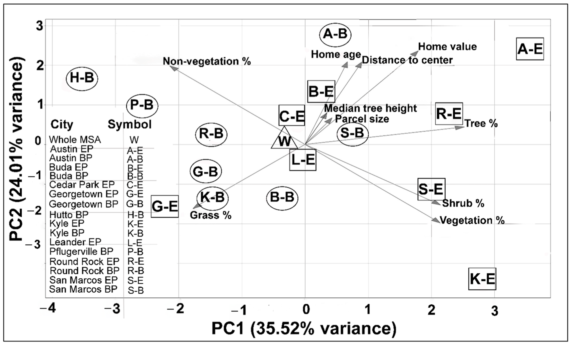
3.4. Variation Among Cities

In an effort to assess vegetation variability among the ten cities and ecoregions, we conducted a PCA. The first two principal components explained almost 60% of the variance among the 16 city–ecoregion combinations (Figure 4). The first principal component (PC1) explained 35.5% of the variance and was largely associated with vegetation metrics (Table 6). Tree cover was the strongest positive loading, followed by shrub cover. The second principal component (PC2) explained 24.0% of the variance and was largely associated with parcel characteristics, particularly home value, home age, and distance to city center.
The PCA of urban vegetation and parcel traits in the Austin MSA showed distinct clustering patterns based on ecoregion characteristics (Figure 4). As expected, the whole MSA (W) was centrally located in the PCA biplot; however, Austin, the largest city and the core of the MSA, was not. Austin was more of an outlier, with stronger associations to parcel characteristics. For most of the other nine cities, the vegetation of the ecoregion drove the separation between clusters, with BP portions of the cities clustering with grass and non-vegetation and EP portions clustering with tree and shrub cover. One notable exception to this pattern was Georgetown-EP (G-E), which clustered with the BP sites.

3.5. City-Scale Variation in Vegetation

Vegetation distribution within the 10 MSA cities revealed mixed results on how parcel characteristics influence tree, shrub, and grass cover (Table 7). Larger parcels generally had higher tree cover in cities like Austin (EP and BP), Round Rock (EP and BP), Georgetown (EP and BP), Cedar Park (EP), and Leander (EP). However, in cities like San Marcos (BP) and Hutto (BP), larger parcels were associated with lower tree cover. Home value played a mixed role. Cities and towns like Austin (EP and BP), San Marcos (EP and BP), Round Rock (BP), Kyle (EP), and Buda (EP) showed that higher home values were linked to more tree cover, while in Round Rock (EP), Georgetown (EP and BP), and Cedar Park (EP), higher values corresponded with lower tree cover. Home age also influenced tree cover, with older homes generally having less tree cover in most cities. In San Marcos (EP), parcels farther from the city center tended to have more tree cover.
Shrub and grass cover showed even more varied relationships. Larger parcels generally resulted in more shrub cover in cities like Austin (EP and BP), San Marcos (EP), Round Rock (EP and BP), and Georgetown (EP), but in San Marcos (BP), Pflugerville (BP), and Hutto (BP), larger parcels were linked to less shrub cover (Table 7). Higher home values had increased shrub cover in cities like Georgetown (EP) and San Marcos (EP) but decreased in other cities. Older homes were generally associated with less shrub cover across most cities, while the distance from the city center influenced shrub cover differently depending on the city. Cities like Austin (EP), San Marcos (EP), Round Rock (BP), Georgetown (BP), and Pflugerville (BP) saw more shrub cover with greater distance, but Kyle (EP and BP) and Austin (BP) saw the opposite, with less shrub cover farther from the center. In most cities, larger parcels had more grass cover. In Austin (EP and BP) and Georgetown (EP), home values showed a positive relationship with grass cover, while in other cities, the relationship was negative.

4. Discussion

4.1. The Role of Physical Geography in Vegetation Structure

This data-intensive and comprehensive study of vegetation distribution across scales within the Austin MSA (Texas, USA) uncovered complex relationships between vegetation structure and human–environment factors from the city to regional scale. Using 1 m-resolution LiDAR data and advanced methods, we created a wall-to-wall 6000 km2 canopy height map for an entire metropolitan region. Post-processing refinements and comparisons with an empirical forest inventory ensured model accuracy, resulting in a detailed and reliable map of vegetation structure. The high-resolution LiDAR data enabled precise classification of vegetation types, while PCA and regression analyses addressed the data structure, revealing the influence of environmental factors on vegetation patterns across scales. Our results highlight the role of biophysical settings in vegetation variation at regional scales as well as socioeconomic factors in shaping urban vegetation.
Vegetation structure is set by physical geography, including climate, soils, and topography [63]. Vegetation structure and distribution across the Austin MSA largely followed the underlying ecoregion characteristics (Figure 3). The Edwards Plateau (EP) ecoregion—characterized by a drier climate, rugged terrain, and shallow calcareous soils—displayed higher (yet patchy) tree and shrub cover. In contrast, the Blackland Prairie (BP) ecoregion—characterized by a slightly wetter climate, relatively flat terrain, and deep productive soils—exhibited a predominance of grass cover and greater areas of non-vegetation cover, with most trees scattered among residential parcels and along riparian areas. Though urbanization does tend to homogenize ecosystem characteristics relative to their native ecoregion [33], the differences in vegetation cover and structure observed in this south–central U.S. region indicate that urbanization is not always intense enough to obscure physical geography signatures.
We did not assess climate change in or the land management history of our study area’s ten cities, but it is likely that these historical changes shaped vegetation patterns [31,64]. Droughts in central Texas have become more frequent, more intense, and longer in duration [65]. When combined with fire hazards, pests (e.g., ash borers), and pathogens (e.g., oak wilt), these climate changes can have devastating effects on the region’s trees. In terms of land management, the rugged EP has historically limited agricultural and urban development, as the slopes discourage building [47]. The flatter, more arable terrain in the BP has been extensively utilized for agriculture and urbanization, and thus likely reduced the prevalence of woody vegetation. In addition, tree planting is a large expense, and urban development on the BP would require substantially more planted trees compared to the EP, with its already-existing or naturally favorable growing conditions.
The topography of each ecoregion also influenced the urban planning and structure that further contributed to the differences in vegetation growth. The EP tended to have larger parcels than the BP. Larger parcel sizes in the EP facilitated the retention of mature, taller vegetation. Tree cover in urban areas often increases with parcel size due to the availability of space for mature vegetation [8]. In contrast, northern BP cities showed reduced tree and shrub cover, reflecting smaller parcel sizes and compact urban development typical of suburban areas. BP cities farther south exhibited higher grass cover, which may be linked to the topography as well as the historical use for farming and ranching.

4.2. Metropolitan-Scale Vegetation Patterns

City-specific patterns in vegetation cover and structure were mostly aligned with ecoregion characteristics (Figure 3); however, we observed significant clustering patterns that revealed a complex pattern across cities (Figure 4). At the city scale, the ecoregion portions of each city clustered together, reflecting the broader pattern of higher tree and shrub cover due to favorable topography and urban design, while BP cities followed the trend of grass dominance and higher non-vegetative cover shaped by agricultural history and rapid urbanization. We observed, however, two notable deviations in some cities. First, both the BP and the EP portion of Austin were more similar than for other cities, where there was higher tree and shrub cover than typical BP cities. This makes vegetation in Austin less similar to its suburbs than they are to each other. This is contrary to initial hypotheses that Austin would be the archetype, with the satellite towns and cities having greater variations [31]. The reasons for Austin’s unique vegetation cover and structure may result from its older age of development and larger population. San Marcos, also one of the older satellite cities, had more similar vegetation distributions between ecoregions (Figure 4). Socioeconomic and management differences may also contribute. In Austin’s core, the higher tree and shrub cover within the BP ecoregion may result from deliberate planting efforts [66]. Human efforts and tree ordinances near the city center may also preserve or increase tree cover at the parcel scale [67,68]. Deliberate urban planning and landscaping efforts in some BP cities may mimic EP-like vegetation characteristics, demonstrating the potential for anthropogenic influence to reshape natural patterns [69,70].
In sum, the regional and city patterns in vegetation cover and structure suggest that urban ecosystems continue to be strongly influenced by their physical geography, but there is significant variability among cities (and likely within cities) that is attributable to socioeconomic factors. In addition, the large core city may be distinct from the surrounding cities and towns that grow and are incorporated into these large MSAs. It is uncertain, however, over time or with population increases, whether these towns will develop vegetation patterns that more closely resemble the core city. These patterns underscore the complex interplay of biophysical and anthropogenic factors shaping urban vegetation across a metropolitan area composed of different-sized cities/towns with different ages [6,31].

4.3. Socioeconomic Factors Affecting Vegetation Distribution

The analysis between parcel characteristics and vegetation metrics revealed significant relationships across the Austin MSA and within cities (Table 3, Table 4, Table 5 and Table 6). It is not surprising, given the differences in cover and structure between the two ecoregions, that socioeconomic factors, though significant, were very weakly correlated with vegetation metrics at the MSA scale (Table 3). However, even when analyzed within an ecoregion, the amount of variation accounted for remained low (Table 4 and Table 5). Socioeconomic factors accounted for more variation in tree cover and height than they did in the percentage of coverage of grass or shrubs at this scale. Home age emerged as the most consistent and influential factor across scales.
Among cities, vegetation characteristics were aligned with certain socioeconomic factors such as home values of each city (Figure 4). High tree and vegetation cover were positively associated with higher home values and larger parcels, consistent with findings from previous studies that link urban greenness with socioeconomic advantages [71]. For instance, neighborhoods with higher home values often have more resources for tree planting and maintenance, contributing to greater canopy cover and biodiversity [72]. This association was particularly evident in the Edwards Plateau portions of the cities, where mature tree cover and larger parcel sizes were prevalent. Conversely, grass cover and non-vegetation percentages were negatively correlated with home values, reflecting patterns of suburban development characterized by compact parcels and reduced investment in landscaping. These findings suggest that socioeconomic factors, in conjunction with ecoregion characteristics, play a crucial role in shaping urban vegetation patterns across the Austin MSA, further emphasizing the need for equitable urban planning to ensure green space access across diverse communities.
When each city was analyzed separately, on the city scale, we found that relationships between factors and vegetation metrics were not uniformly consistent among the cities (Table 7). The most consistent relationship we observed was between home age and tree cover, which was negatively correlated for all ten cities. Home value was also significantly related to parcel tree cover for all ten cities, but large cities had negative correlations, while small cities had positive correlations. Parcel size and distance were significant for some cities and vegetation types, but inconsistently so. We observed no clear pattern in those results; however, we did observe that for the larger cities, Austin and Round Rock, more of the factors were significant. In small cities, fewer factors tended to be significant. It is possible that this finding resulted from differences in the number of parcels. Alternatively, as cities grow, there may be more opportunity for differentiation in vegetation structure along these different socioeconomic factors, creating a more complex mosaic.
Home age and value were the most consistent factors among the cities. Home age was negatively correlated with tree cover, median tree height, and overall vegetation cover. This suggests that older homes are generally situated in areas with less vegetation, potentially due to historical urban development practices and limited space for vegetation retention or growth over time. The relationship with home age and tree cover has been found to be inconsistent in other studies. In Baltimore (Maryland, USA), tree cover increased up to 45 to 50 years, then declined with age [73,74]. In Phoenix, the opposite was observed, where urban vegetation abundance in neighborhoods declined from 0 to 50 years of age [75,76]. Austin cities are also located in a drier climate and are consistent with findings from Phoenix. A positive relationship between tree cover and home values suggests that while individual property owners and buyers often value tree cover, its impact on broader market trends can be influenced by a variety of other factors [77,78,79]. Several studies found extensive urbanization pressures to be a main factor, where higher land values lead to more intensive development, potentially at the expense of existing vegetation cover [80,81].
Overall, our findings reveal the interplay between physical geography and urban development influences in shaping vegetation patterns. While parcel traits like home age, parcel size, and home value influence vegetation coverage, the underlying ecoregion remains a dominant driver. The distinction between the EP’s tree-dominated landscape and the BP’s grass-centric patterns highlights the importance of considering biophysical factors alongside anthropogenic influences in urban vegetation studies. These insights underscore the need for context-sensitive planning strategies that integrate native vegetation dynamics with urban design to enhance ecological and social benefits across diverse ecoregions.

5. Conclusions

Vegetation structure, including types, height, and area, showed uneven distributions across scales of space and time. Physical geography factors associated with ecoregion differences influenced spatial patterns across parcels, neighborhoods, and cities. Vegetation distribution was also dependent on parcel characteristics, such as the home’s size, age, value, and proximity to city centers. Across the 6000 km2 metropolitan region, there were significant variations in vegetation distribution across ecoregions and among cities. The Edwards Plateau (EP) ecoregion had higher tree and shrub coverage compared to the Blackland Prairie (BP), where grass cover was more dominant. Among the 10 cities, parcel characteristics such as lot size, home value, home age, and distance to city center were found to have varying relationships with different types of vegetation, indicating that larger, older, and more valuable parcels generally supported more trees, although these trends varied by ecoregion and scale.
Though this study comprehensively analyzed vegetation cover and parcel characteristics across scales, future studies should incorporate socioeconomic variables such as income, property ownership types, and demographic data to understand the social determinants of vegetation distribution. All of these issues are important to improving wildlife habitat, enhancing human wellbeing, and addressing environmental injustices [11,82]. While our study did not assess the volumetric structure of vegetation, incorporating vegetation volume measurements could improve our understanding of urban vegetation with a more detailed assessment of biomass, carbon storage, habitat, and overall ecological value [83]. Analyzing tree volume alongside height and area would provide a more comprehensive view of vegetation structure and distribution, enabling informed urban planning and conservation strategies [84]. Therefore, future studies should aim to include vegetation volume functions and socioeconomic factors to deepen our understanding of urban ecosystems and their contributions to ecosystem services and overall wellbeing.

Author Contributions

Conceptualization, R.J., J.P.J. and M.K.S.; methodology, R.J., J.P.J. and M.K.S.; software, R.J.; validation, R.J., J.P.J. and M.K.S.; formal analysis, R.J.; investigation, R.J., J.P.J. and M.K.S.; resources, R.J. and J.P.J.; data curation, R.J.; writing—original draft preparation, R.J., J.P.J. and M.K.S.; writing—review and editing, R.J., J.P.J. and M.K.S.; visualization, R.J.; supervision, J.P.J.; project administration, J.P.J. All authors have read and agreed to the published version of the manuscript.

Funding

This research received no external funding.

Data Availability Statement

This study utilized publicly available data from multiple sources, including LiDAR point cloud data and imagery from the USGS 3D Elevation Program, census data, and CAD data from county offices. All datasets were processed and analyzed to derive the reported results. The first author can provide access to specific processed datasets upon request, subject to privacy and ethical considerations.

Acknowledgments

We thank Jennifer Jensen and the two anonymous reviewers, whose advice and comments improved this manuscript.

Conflicts of Interest

The authors declare no conflicts of interest.

References

  1. Cousins, S.A.; Auffret, A.G.; Lindgren, J.; Tränk, L. Regional-scale land-cover change during the 20th century and its consequences for biodiversity. Ambio 2015, 44, 17–27. [Google Scholar] [CrossRef]
  2. Lambin, E.F.; Geist, H.J. Land-Use and Land-Cover Change: Local Processes and Global Impacts; Springer Science & Business Media: Heidelburg, Germany, 2008; pp. 9–15. [Google Scholar]
  3. Vitousek, P.M. Beyond global warming: Ecology and global change. Ecology 1994, 75, 1861–1876. [Google Scholar] [CrossRef]
  4. Brunner, J.; Cozens, P. ‘Where have all the trees gone?’Urban consolidation and the demise of urban vegetation: A case study from Western Australia. Plan. Pract. Res. 2013, 28, 231–255. [Google Scholar] [CrossRef]
  5. Fuller, R.A.; Gaston, K.J. The scaling of green space coverage in European cities. Biol. Lett. 2009, 5, 352–355. [Google Scholar] [CrossRef] [PubMed]
  6. Qian, Y.; Zhou, W.; Li, W.; Han, L. Understanding the dynamic of greenspace in the urbanized area of Beijing based on high resolution satellite images. Urban For. Urban Green. 2015, 14, 39–47. [Google Scholar] [CrossRef]
  7. Yu, Z.; Wang, Y.; Deng, J.; Shen, Z.; Wang, K.; Zhu, J.; Gan, M. Dynamics of hierarchical urban green space patches and implications for management policy. Sensors 2017, 17, 1304. [Google Scholar] [CrossRef]
  8. Zhou, W.; Wang, J.; Cadenasso, M.L. Effects of the spatial configuration of trees on urban heat mitigation: A comparative study. Remote Sens. Environ. 2017, 195, 43. [Google Scholar] [CrossRef]
  9. Lo, A.Y.; Jim, C.Y. Differential community effects on perception and use of urban greenspaces. Cities 2010, 27, 430–442. [Google Scholar] [CrossRef]
  10. Sivam, A.; Karuppannan, S.; Mobbs, M. How “open” are open spaces: Evaluating transformation of open space at residential level in Adelaide–a case study. Local Environ. 2012, 17, 815–836. [Google Scholar] [CrossRef]
  11. Wolch, J.R.; Byrne, J.; Newell, J.P. Urban green space, public health, and environmental justice: The challenge of making cities ‘just green enough’. Landsc. Urban Plan. 2014, 125, 234–244. [Google Scholar] [CrossRef]
  12. He, C.; Liu, Z.; Gou, S.; Zhang, Q.; Zhang, J.; Xu, L. Detecting global urban expansion over the last three decades using a fully convolutional network. Environ. Res. Lett. 2019, 14, 034008. [Google Scholar] [CrossRef]
  13. Pregitzer, C.C.; Ashton, M.S.; Charlop-Powers, S.; D’Amato, A.W.; Frey, B.R.; Gunther, B.; Hallett, R.A.; Pregitzer, K.S.; Woodall, C.W.; Bradford, M.A. Defining and assessing urban forests to inform management and policy. Environ. Res. Lett. 2019, 14, 085002. [Google Scholar] [CrossRef]
  14. Benn, S.; Gaus, G. Public and Private in Social Life; Croom Helm: London, UK, 1983; pp. 121–125. [Google Scholar]
  15. Madanipour, A. Why are the design and development of public spaces significant for cities? Environ. Plan. B Plan. Des. 1999, 26, 879–891. [Google Scholar] [CrossRef]
  16. Steenberg, J.W.; Millward, A.A.; Duinker, P.N.; Nowak, D.J.; Robinson, P.J. Neighbourhood-scale urban forest ecosystem classification. J. Environ. Manag. 2015, 163, 134–145. [Google Scholar] [CrossRef]
  17. Jamil, R.; Julian, J.P.; Jensen, J.L.; Meitzen, K.M. Urban Green Infrastructure Connectivity: The Role of Private Semi-Natural Areas. Land 2024, 13, 1213. [Google Scholar] [CrossRef]
  18. Harris, V.; Kendal, D.; Hahs, A.K.; Threlfall, C.G. Green space context and vegetation complexity shape people’s preferences for urban public parks and residential gardens. Landsc. Res. 2018, 43, 150–162. [Google Scholar] [CrossRef]
  19. Goddard, M.A.; Dougill, A.J.; Benton, T.G. Scaling up from gardens: Biodiversity conservation in urban environments. Trends Ecol. Evol. 2010, 25, 90–98. [Google Scholar] [CrossRef]
  20. Belaire, J.A.; Whelan, C.J.; Minor, E.S. Having our yards and sharing them too: The collective effects of yards on native bird species in an urban landscape. Ecol. Appl. 2014, 24, 2132–2143. [Google Scholar] [CrossRef]
  21. Paker, Y.; Yom-Tov, Y.; Alon-Mozes, T.; Barnea, A. The effect of plant richness and urban garden structure on bird species richness, diversity and community structure. Landsc. Urban Plan. 2014, 122, 186–195. [Google Scholar] [CrossRef]
  22. Vergnes, A.; Le Viol, I.; Clergeau, P. Green corridors in urban landscapes affect the arthropod communities of domestic gardens. Biol. Conserv. 2012, 145, 171–178. [Google Scholar] [CrossRef]
  23. Casalegno, S.; Anderson, K.; Cox, D.T.; Hancock, S.; Gaston, K.J. Ecological connectivity in the three-dimensional urban green volume using waveform airborne lidar. Sci. Rep. 2017, 7, 45571. [Google Scholar] [CrossRef]
  24. Ossola, A.; Hopton, M.E. Measuring urban tree loss dynamics across residential landscapes. Sci. Total Environ. 2018, 612, 940–949. [Google Scholar] [CrossRef] [PubMed]
  25. Mitchell, M.G.; Bennett, E.M.; Gonzalez, A. Linking landscape connectivity and ecosystem service provision: Current knowledge and research gaps. Ecosystems 2013, 16, 894–908. [Google Scholar] [CrossRef]
  26. Kolbe, J.J.; VanMiddlesworth, P.; Battles, A.C.; Stroud, J.T.; Buffum, B.; Forman, R.T.; Losos, J.B. Determinants of spread in an urban landscape by an introduced lizard. Landsc. Ecol. 2016, 31, 1795–1813. [Google Scholar] [CrossRef]
  27. Treby, D.L.; Castley, J.G. Distribution and abundance of hollow-bearing trees in urban forest fragments. Urban For. Urban Green. 2015, 14, 655–663. [Google Scholar] [CrossRef]
  28. Stagoll, K.; Lindenmayer, D.B.; Knight, E.; Fischer, J.; Manning, A.D. Large trees are keystone structures in urban parks. Conserv. Lett. 2012, 5, 115–122. [Google Scholar] [CrossRef]
  29. Fontana, S.; Sattler, T.; Bontadina, F.; Moretti, M. How to manage the urban green to improve bird diversity and community structure. Landsc. Urban Plan. 2011, 101, 278–285. [Google Scholar] [CrossRef]
  30. Savard, J.-P.L.; Clergeau, P.; Mennechez, G. Biodiversity concepts and urban ecosystems. Landsc. Urban Plan. 2000, 48, 131–142. [Google Scholar] [CrossRef]
  31. Forman, R.T. Towns, Ecology, and the Land; Cambridge University Press: Cambridge, UK, 2019; pp. 9–18. [Google Scholar]
  32. Dobbs, C.; Nitschke, C.; Kendal, D. Assessing the drivers shaping global patterns of urban vegetation landscape structure. Sci. Total Environ. 2017, 592, 171–177. [Google Scholar] [CrossRef]
  33. Groffman, P.M.; Cavender-Bares, J.; Bettez, N.D.; Grove, J.M.; Hall, S.J.; Heffernan, J.B.; Hobbie, S.E.; Larson, K.L.; Morse, J.L.; Neill, C. Ecological homogenization of urban USA. Front. Ecol. Environ. 2014, 12, 74–81. [Google Scholar] [CrossRef]
  34. Steele, M.; Wolz, H. Heterogeneity in the land cover composition and configuration of US cities: Implications for ecosystem services. Landsc. Ecol. 2019, 34, 1247–1261. [Google Scholar] [CrossRef]
  35. Cox, L.; Hansen, V.; Andrews, J.; Thomas, J.; Heilke, I.; Flanders, N.; Walton, B. Land Use: A Powerful Determinant of Sustainable & Healthy Communities; US Environmental Protection Agency: Washington, DC, USA, 2013. Available online: https://www.epa.gov/sites/default/files/2016-09/documents/fy13productnheerl4121land_use_synthesis.pdf (accessed on 25 February 2024).
  36. McDonald, R.I.; Biswas, T.; Chakraborty, T.; Kroeger, T.; Cook-Patton, S.C.; Fargione, J.E. Current inequality and future potential of US urban tree cover for reducing heat-related health impacts. NPJ Urban Sustain. 2024, 4, 18. [Google Scholar] [CrossRef]
  37. Ziter, C.D.; Pedersen, E.J.; Kucharik, C.J.; Turner, M.G. Scale-dependent interactions between tree canopy cover and impervious surfaces reduce daytime urban heat during summer. Proc. Natl. Acad. Sci. USA 2019, 116, 7575–7580. [Google Scholar] [CrossRef] [PubMed]
  38. Nowak, D.J.; Greenfield, E.J. Tree and impervious cover in the United States. Landsc. Urban Plan. 2012, 107, 21–30. [Google Scholar] [CrossRef]
  39. Locke, D.H.; Hall, B.; Grove, J.M.; Pickett, S.T.; Ogden, L.A.; Aoki, C.; Boone, C.G.; O’Neil-Dunne, J.P. Residential housing segregation and urban tree canopy in 37 US Cities. NPJ Urban Sustain. 2021, 1, 15. [Google Scholar] [CrossRef]
  40. Liu, H.; Dong, P. A new method for generating canopy height models from discrete-return LiDAR point clouds. Remote Sens. Lett. 2014, 5, 575–582. [Google Scholar] [CrossRef]
  41. Kulawardhana, R.W.; Popescu, S.C.; Feagin, R.A. Fusion of lidar and multispectral data to quantify salt marsh carbon stocks. Remote Sens. Environ. 2014, 154, 345–357. [Google Scholar] [CrossRef]
  42. Hartfield, K.A.; Landau, K.I.; Van Leeuwen, W.J. Fusion of high resolution aerial multispectral and LiDAR data: Land cover in the context of urban mosquito habitat. Remote Sens. 2011, 3, 2364–2383. [Google Scholar] [CrossRef]
  43. MacFaden, S.W.; O′Neil-Dunne, J.P.; Royar, A.R.; Lu, J.W.; Rundle, A.G. High-resolution tree canopy mapping for New York City using LIDAR and object-based image analysis. J. Cell. Physiol. 2012, 6, 063567. [Google Scholar] [CrossRef]
  44. Data USA. San Marcos, TX. Available online: https://datausa.io/profile/geo/san-marcos-tx/ (accessed on 29 August 2024).
  45. Service, N.W. Austin Climate Summary. Available online: https://www.weather.gov/media/ewx/climate/ClimateSummary-ewx-Austin.pdf (accessed on 29 August 2024).
  46. TPWD, T.P.A.W. By Ecoregion (Vector). Available online: https://tpwd.texas.gov/gis/programs/landscape-ecology/by-ecoregion-vector (accessed on 29 August 2023).
  47. Chapman, B.R.; Bolen, E.G. The Natural History of the Edwards Plateau: The Texas Hill Country; Texas A&M University Press: College Station, TX, USA, 2020; pp. 51–55. [Google Scholar]
  48. Diamond, D.D.; Smeins, F.E. Composition, classification and species response patterns of remnant tallgrass prairies in Texas. Am. Midl. Nat. 1985, 113, 294–308. [Google Scholar] [CrossRef]
  49. Heidemann, H.K. Lidar Base Specification; 2328-7055; US Geological Survey: Washington, DC, USA, 2012; pp. 41–42.
  50. Jamil, R. Social Demands and Geospatial Distributions of Urban Green Spaces and Blue Spaces. Ph.D. Dissertation, Texas State University, San Marcos, TX, USA, 2024. Available online: https://digital.library.txst.edu/items/0e6cd5d2-8801-4370-b427-c7e1d0d8d551/full (accessed on 28 February 2025).
  51. Jennings, S.; Brown, N.; Sheil, D. Assessing Forest Canopies and Understorey Illumination: Canopy Closure, Canopy Cover and Other Measures; Oxford University Press: Oxford, UK, 1999; Volume 72, pp. 59–74. [Google Scholar] [CrossRef]
  52. Hermansen-Baez, A. Urban Tree Canopy Assessment: A Community’s Path to Understanding and Managing the Urban Forest; FS-1121; U.S. Department of Agriculture, Forest Service: Washington, DC, USA, 2019; pp. 1–16.
  53. Brokaw, N.V. The definition of treefall gap and its effect on measures of forest dynamics. Biotropica 1982, 14, 158–160. [Google Scholar] [CrossRef]
  54. Ucar, Z.; Bettinger, P.; Merry, K.; Akbulut, R.; Siry, J. Estimation of Urban Woody Vegetation Cover Using Multispectral Imagery and LiDAR; Elsevier: Amsterdam, The Netherlands, 2018; Volume 29, pp. 248–260. [Google Scholar] [CrossRef]
  55. Weinstein, B.G.; Marconi, S.; Bohlman, S.A.; Zare, A.; Singh, A.; Graves, S.J.; White, E.P. A Remote Sensing Derived Data Set of 100 Million Individual Tree Crowns for the National Ecological Observatory Network; eLife Sciences Publications, Ltd.: Zurich, Switzerland, 2021; Volume 10. [Google Scholar] [CrossRef]
  56. Salmond, J.A.; Tadaki, M.; Vardoulakis, S.; Arbuthnott, K.; Coutts, A.; Demuzere, M.; Dirks, K.N.; Heaviside, C.; Lim, S.; Macintyre, H. Health and climate related ecosystem services provided by street trees in the urban environment. Environ. Health 2016, 15, 95–111. [Google Scholar] [CrossRef] [PubMed]
  57. Dai, X.; Li, Z.; Lin, S.; Xu, W. Assessment and zoning of eco-environmental sensitivity for a typical developing province in China. Stoch. Environ. Res. Risk Assess. 2012, 26, 1095–1107. [Google Scholar] [CrossRef]
  58. Cook, E.M.; Hall, S.J.; Larson, K.L. Residential landscapes as social-ecological systems: A synthesis of multi-scalar interactions between people and their home environment. Urban Ecosyst. 2012, 15, 19–52. [Google Scholar] [CrossRef]
  59. Pickett, S.T.; Cadenasso, M.L.; Grove, J.M.; Boone, C.G.; Groffman, P.M.; Irwin, E.; Kaushal, S.S.; Marshall, V.; McGrath, B.P.; Nilon, C.H. Urban ecological systems: Scientific foundations and a decade of progress. J. Environ. Manag. 2011, 92, 331–362. [Google Scholar] [CrossRef] [PubMed]
  60. Smith, R.M.; Gaston, K.J.; Warren, P.H.; Thompson, K. Urban domestic gardens (V): Relationships between landcover composition, housing and landscape. Landsc. Ecol. 2005, 20, 235–253. [Google Scholar] [CrossRef]
  61. Verbeeck, K.; Van Orshoven, J.; Hermy, M. Measuring extent, location and change of imperviousness in urban domestic gardens in collective housing projects. Landsc. Urban Plan. 2011, 100, 57–66. [Google Scholar] [CrossRef]
  62. Breen, R. Regression Models: Censored, Sample Selected, or Truncated Data; Sage: Riverside County, CA, USA, 1996; pp. 12–18. [Google Scholar]
  63. Omernik, J.M.; Griffith, G.E. Ecoregions of the conterminous United States: Evolution of a hierarchical spatial framework. Environ. Manag. 2014, 54, 1249–1266. [Google Scholar] [CrossRef]
  64. Wilcox, B.P.; Sorice, M.G.; Young, M.H. Dryland ecohydrology in the anthropocene: Taking stock of human–ecological interactions. Geogr. Compass 2011, 5, 112–127. [Google Scholar] [CrossRef]
  65. Nielsen-Gammon, J.W.; Banner, J.L.; Cook, B.I.; Tremaine, D.M.; Wong, C.I.; Mace, R.E.; Gao, H.; Yang, Z.L.; Gonzalez, M.F.; Hoffpauir, R. Unprecedented drought challenges for Texas water resources in a changing climate: What do researchers and stakeholders need to know? Earth′s Future 2020, 8, e2020EF001552. [Google Scholar] [CrossRef]
  66. Willis, E.M.; Koeser, A.K.; Clarke, M.; Hansen, G.; Hilbert, D.R.; Lusk, M.G.; Roman, L.A.; Warner, L.A. Greening development: Reducing urban tree canopy loss through incentives. Urban For. Urban Green. 2024, 91, 128184. [Google Scholar] [CrossRef]
  67. Lavy, B.L.; Hagelman III, R.R. Protecting the urban forest: Variations in standards and sustainability dimensions of municipal tree preservation ordinances. Urban For. Urban Green. 2019, 44, 126394. [Google Scholar] [CrossRef]
  68. Larson, K.L.; Andrade, R.; Nelson, K.C.; Wheeler, M.M.; Engebreston, J.M.; Hall, S.J.; Avolio, M.L.; Groffman, P.M.; Grove, M.; Heffernan, J.B. Municipal regulation of residential landscapes across US cities: Patterns and implications for landscape sustainability. J. Environ. Manag. 2020, 275, 111132. [Google Scholar] [CrossRef] [PubMed]
  69. Jim, C.Y. Green-space preservation and allocation for sustainable greening of compact cities. Cities 2004, 21, 311–320. [Google Scholar] [CrossRef]
  70. Tan, P.Y.; Wang, J.; Sia, A. Perspectives on five decades of the urban greening of Singapore. Cities 2013, 32, 24–32. [Google Scholar] [CrossRef]
  71. Escobedo, F.J.; Kroeger, T.; Wagner, J.E. Urban forests and pollution mitigation: Analyzing ecosystem services and disservices. Environ. Pollut. 2011, 159, 2078–2087. [Google Scholar] [CrossRef]
  72. Jim, C.Y.; Shan, X. Socioeconomic effect on perception of urban green spaces in Guangzhou, China. Cities 2013, 31, 123–131. [Google Scholar] [CrossRef]
  73. Morgan Grove, J.; Cadenasso, M.L.; Burch Jr, W.R.; Pickett, S.T.; Schwarz, K.; O′Neil-Dunne, J.; Wilson, M.; Troy, A.; Boone, C. Data and methods comparing social structure and vegetation structure of urban neighborhoods in Baltimore, Maryland. Soc. Nat. Resour. 2006, 19, 117–136. [Google Scholar] [CrossRef]
  74. Troy, A.R.; Grove, J.M.; O’Neil-Dunne, J.P.; Pickett, S.T.; Cadenasso, M.L. Predicting opportunities for greening and patterns of vegetation on private urban lands. Environ. Manag. 2007, 40, 394–412. [Google Scholar] [CrossRef]
  75. Hope, D.; Gries, C.; Zhu, W.; Fagan, W.F.; Redman, C.L.; Grimm, N.B.; Nelson, A.L.; Martin, C.; Kinzig, A. Socioeconomics drive urban plant diversity. Proc. Natl. Acad. Sci. USA 2003, 100, 8788–8792. [Google Scholar] [CrossRef]
  76. Martin, C.A.; Warren, P.S.; Kinzig, A.P. Neighborhood socioeconomic status is a useful predictor of perennial landscape vegetation in residential neighborhoods and embedded small parks of Phoenix, AZ. Landsc. Urban Plan. 2004, 69, 355–368. [Google Scholar] [CrossRef]
  77. Escobedo, F.J.; Adams, D.C.; Timilsina, N. Urban forest structure effects on property value. Ecosyst. Serv. 2015, 12, 209–217. [Google Scholar] [CrossRef]
  78. Sayler, K.L.; Acevedo, W.; Taylor, J.L. Status and trends of land change in selected US ecoregions-2000 to 2011. Photogramm. Eng. Remote Sens. 2016, 82, 687–697. [Google Scholar] [CrossRef]
  79. Kovacs, K.; West, G.; Nowak, D.J.; Haight, R.G. Tree cover and property values in the United States: A national meta-analysis. Ecol. Econ. 2022, 197, 107424. [Google Scholar] [CrossRef]
  80. Seto, K.C.; Sánchez-Rodríguez, R.; Fragkias, M. The new geography of contemporary urbanization and the environment. Annu. Rev. Environ. Resour. 2010, 35, 167–194. [Google Scholar] [CrossRef]
  81. Eigenbrod, F.; Bell, V.; Davies, H.; Heinemeyer, A.; Armsworth, P.R.; Gaston, K.J. The impact of projected increases in urbanization on ecosystem services. Proc. R. Soc. B Biol. Sci. 2011, 278, 3201–3208. [Google Scholar] [CrossRef]
  82. Sandifer, P.A.; Sutton-Grier, A.E.; Ward, B.P. Exploring connections among nature, biodiversity, ecosystem services, and human health and well-being: Opportunities to enhance health and biodiversity conservation. Ecosyst. Serv. 2015, 12, 1–15. [Google Scholar] [CrossRef]
  83. Davies, Z.G.; Edmondson, J.L.; Heinemeyer, A.; Leake, J.R.; Gaston, K.J. Mapping an urban ecosystem service: Quantifying above-ground carbon storage at a city-wide scale. J. Appl. Ecol. 2011, 48, 1125–1134. [Google Scholar] [CrossRef]
  84. Bergen, K.; Goetz, S.; Dubayah, R.; Henebry, G.; Hunsaker, C.; Imhoff, M.; Nelson, R.; Parker, G.; Radeloff, V. Remote sensing of vegetation 3-D structure for biodiversity and habitat: Review and implications for lidar and radar spaceborne missions. J. Geophys. Res. Biogeosciences 2009, 114, 883. [Google Scholar] [CrossRef]
Figure 1. Study area covering the Austin Metropolitan Statistical Area (MSA), including Austin in the center and nine other cities. The MSA lays on the border of an ecoregion boundary (yellow line), with the Edwards Plateau (EP) to the west and the Blackland Prairie (BP) to the east.
Geographies 05 00011 g001
Figure 2. An example neighborhood in Austin, Texas, USA, that shows the overlay of individual parcel boundaries on vegetation classes (tree, shrub, and grass) derived from a LiDAR-based canopy height model (CHM).
Geographies 05 00011 g002
Figure 3. Austin MSA vegetation map (grass, shrub, and tree cover) derived from the canopy height model (CHM) for the year 2020. Statistical distributions of vegetation cover in the right margin comparing the Edwards Plateau (EP) ecoregion to the west and the Blackland Prairie (BP) ecoregion to the east. An unpaired t-test was used for normally distributed variables (grass cover, shrub cover, and median tree height), while the Mann–Whitney test was applied to zero-inflated distributions (tree cover).
Geographies 05 00011 g003
Figure 4. Principal component analysis (PCA) of vegetation metrics and parcel characteristics across cities (first letter) and ecoregions (second letter and symbol) in the Austin MSA.
Geographies 05 00011 g004
Table 1. Vegetation structure metrics and parcel characteristics selected for analyses and comparisons.
Vegetation MetricsParcel Characteristics
Vegetation cover by type: grass (%), shrub (%), tree (%)
Median tree height (meters)
Parcel size (ha)
Distance to city center (km)
Home age (years since construction)
Maximum tree height (meters) Home value (2020 market price in USD)
Total vegetation cover (%)
Non-vegetation cover (%)
Table 2. Summary statistics of MSA city parcel characteristics, separated by the Edwards Plateau (EP) and the Blackland Prairie (BP) ecoregions.
NameEcoregionNumber of ParcelsMedian Parcel Size (ha)Median Home Value (USD)Median Distance to City Center (km)Median Age2020 City Population
AustinEP246,3470.09476,96914.8129974,000
BP0.07366,1067.5249
BudaEP94290.09301,38011.651016,000
BP0.09234,32010.2713
Cedar ParkEP15,7440.10289,5875.241677,000
GeorgetownEP15,9870.15314,5084.551586,000
BP0.10223,1736.3315
HuttoBP53900.10217,5722.421436.000
KyleEP18,4510.07236,1903.181157,000
BP0.07216,4703.1815
LeanderEP18,1670.10291,4165.331674,000
PflugervilleBP11,4270.08244,8034.032165,000
Round RockEP35,7650.12304,4924.6916126,000
BP0.11208,0303.347
San MarcosEP14,9030.10241,9902.742168,000
BP0.08168,4903.4817
Entire MSAEP391,6100.10307,0675.23172,176,000
BP0.09234,8713.9220
Table 3. Correlation matrix among all variables at the MSA scale for Austin, TX. Bold values are significant at p < 0.05.
Parcel SizeHome AgeHome ValueDistance to City CenterMedian Tree HeightGrass CoverShrub CoverTree CoverTotal Vegetation
Parcel size1−0.310.070.04−0.010.030.020.0080.04
Home age 1−0.10−0.01−0.310.310.29−0.2−0.41
Home value 1−0.140.14−0.130.030.220.16
Distance to city center 1−0.100.230.04−0.120.03
Median tree height 1−0.31−0.270.630.36
Grass cover 1−0.08−0.520.08
Shrub cover 10.140.51
Tree cover 10.73
Total vegetation 1
Table 4. Parcel-scale stepwise regression models of vegetation metrics and parcel characteristics for Austin MSA parcels in the Edwards Plateau (EP) ecoregion. Only variables with significant r values are shown.
Vegetation CharacteristicsStepParcel CharacteristicsMultivariate Sequential r2AICBivariate r
Tree cover(%)1Home age 0.2941129318−0.542
2Home value 0.30111279820.134
3Distance to city center 0.30211278450.093
4Parcel size 0.30211278420.013
Shrub cover (%)1Home value 0.002921614−0.048
2Parcel size 0.0039214670.032
3Distance to city center 0.004921439−0.019
Grass cover
(%)
1Home age 0.08810119180.296
2Distance to city center 0.0931011213−0.103
3Home value 0.0931011097−0.060
4Parcel size 0.09410109730.020
Median tree height (m)1Home age 0.114382953−0.337
2Distance to city center 0.1193822260.108
3Home value 0.1233816520.097
4Parcel size 0.123381631−0.001
Table 5. Parcel-scale stepwise regression models of vegetation metrics and parcel characteristics for Austin MSA parcels in the Blackland Prairie (BP) ecoregion. Only variables with significant r values are shown.
Vegetation CharacteristicsStepParcel CharacteristicsMultivariate Sequential r2AICBivariate r
Tree cover
(%)
1Home age 0.3011039880−0.549
2Home value 0.31810369340.273
3Distance to city center 0.3221036310−0.079
4Parcel size 0.3231036075−0.036
Shrub cover (%)1Home age 0.050839288−0.224
2Home value 0.062837778−0.044
3Distance to city center 0.0638376380.001
4Parcel size 0.063837625−0.014
Grass cover
(%)
1Home age 0.0899662840.299
2Parcel size 0.1109634910.148
3Home value 0.132960557−0.218
4Distance to city center 0.1329605280.108
Median tree height (m)1Home age 0.128381141−0.357
2Home value 0.1473784840.229
3Distance to city center 0.153377553−0.018
4Parcel size 0.154377476−0.019
Table 6. Principal component analysis (PCA) loadings for vegetation metrics and parcel characteristics in the Austin MSA. Bold values have an absolute correlation coefficient (|r|) greater than 0.2.
VariablePC1PC2
Home value 0.170.24
Home age 0.070.22
Parcel size 0.040.07
Distance to city center0.090.22
Median tree height0.030.08
Grass %−0.17−0.16
Shrub %0.24−0.16
Tree %0.270.06
Vegetation %0.23−0.20
Non-vegetation %0.230.20
Table 7. Multiple regression model variable coefficients for vegetation structure (percent tree, shrub, and grass cover) and residential parcel characteristics (size, home value, home age, and distance to city center). Results are presented for portions of the city in each ecoregion, the Edwards Plateau (EP) and Blackland Prairie (BP). Cities are arranged by city population for 2024. Green cells indicate a significant relationship with p < 0.05.
Large Cities (>100,000)Medium Cities
(50,000–100,000)
Small Cities
(<50,000)
AustinRound RockGeorgetownCedar Park Leander San MarcosPflugervilleKyle HuttoBuda
EP (Tree)Parcel size 4.6 × 10−50.0010.0010.0015.6 × 10−4−3 × 10⁻⁶No EP−0.235No EP1.3 × 10−5
Home value 2 × 10⁻⁷−1 × 10⁻⁶−5 × 10⁻⁶−4 × 10⁻⁶−4 × 10−63 × 10−61 × 10−54.4 × 10−6
Home age −0.611−0.776−0.566−0.9−0.900−0.152−0.10−5−1.114
Distance −0.0011 × 10−54 × 10−5−6 × 10⁶−6 × 10−60.001−6 × 10⁻⁴−8 × 10⁻⁴
BP (Tree) Parcel size 1 × 10−41 × 10−41 × 10−4No BPNo BP−2 × 10−40.003−1 × 10⁻⁶−5 × 10−51 × 10−5
Home value 2 × 10−71 × 10−6−3 × 10−61 × 10−6−8 × 10−74 × 10−7−2 × 10−74 × 10−6
Home age −0.002−0.281−0.164−0.346−1.117−0.692−0.153−1.114
Distance 1 × 10⁻⁵−1 × 10⁻⁶−7 × 10⁻⁵−0.0010.002−0.0012 × 10⁻⁵−0.001
EP (Shrub)Parcel size 2 × 10−71 × 10−40.0010.0012 × 1046 × 10−6No EP6 × 10−7No EP−6 × 10⁻⁵
Home value−0.477−1 × 10−65 × 10−7−2 × 10⁻⁴−2 × 10−44 × 10−72 × 10−6−8 × 10⁻⁷
Home age 1 × 10⁻⁴−0.346−0.221−0.356−0.3560.009−0.007−0.355
Distance 1 × 10−41 × 10−5−1 × 10−51 × 10−51 × 10−55 × 10−5−4 × 10⁻⁴−5 × 10⁻⁵
BP (Shrub)Parcel size 5 × 10−51 × 10−4−3 × 10⁻⁵No BPNo BP−1 × 10⁻⁴−3 × 10⁻⁴−3 × 10⁻⁶−0.001−6 × 10⁻⁵
Home value −5 × 10⁻⁶−2 × 10⁻⁷−4 × 10⁻⁶−2 × 10−64 × 10−7−5 × 10−71 × 10−7−8 × 10⁻⁷
Home age −0.088−0.155−0.161−0.054−0.256−0.477−0.289−0.355
Distance−8 × 10−51 × 10−51 × 10−4−2 × 10−55 × 10−5−7 × 10⁻⁴−1 × 10⁻⁵−5 × 10⁻⁵
EP (Grass)Parcel size 9 × 10−50.0011 × 10−50.0010.0015 × 10−5No EP−4 × 10⁻⁷No EP8 × 10−4
Home value 2 × 10⁻⁷−2 × 10−66 × 10−6−2 × 10⁻⁶−2 × 10−63 × 10−8−1 × 10⁻⁵−8 × 10⁻⁷
Home age 0.1790.3690.060.2880.289−0.0770.046−0.222
Distance 6 × 10⁻⁵−2 × 10⁻⁵−2 × 10⁻⁵−3 × 10⁻⁶−3 × 10⁻⁶−1 × 10−46 × 10−46 × 10−4
BP (Grass)Parcel size 0.0011 × 10−40.001No BPNo BP6 × 10−42 × 10−41 × 10−4−0.0010.001
Home value 5 × 10⁻⁶−2 × 10⁻⁷−1 × 10−57 × 10−7−3 × 10−64 × 10−7−2 × 10⁻⁶−8 × 10⁻⁷
Home age 0.075−0.1550.1010.1418−7.035−0.1070.148−0.222
Distance 1 × 10−41 × 10−51 × 10−40.003−6 × 1050.0020.0010.001
Disclaimer/Publisher’s Note: The statements, opinions and data contained in all publications are solely those of the individual author(s) and contributor(s) and not of MDPI and/or the editor(s). MDPI and/or the editor(s) disclaim responsibility for any injury to people or property resulting from any ideas, methods, instructions or products referred to in the content.

