Article

A Swap-Body Vehicle Routing Problem Considering Fuel Consumption Management and Multiple Vehicle Trips

1
School of Traffic and Transportation, Chongqing Jiaotong University, Chongqing 400074, China
2
The David D. Reh School of Business, Clarkson University, Potsdam, NY 13699, USA
3
Chongqing Jiangjin District Road Transportation Affairs Center, Chongqing 402218, China
4
Macquarie Business School, Macquarie University, Sydney 2109, Australia
*
Author to whom correspondence should be addressed.
Future Transp. 2024, 4(3), 1000-1021; https://doi.org/10.3390/futuretransp4030048
Submission received: 1 July 2024 / Revised: 26 August 2024 / Accepted: 2 September 2024 / Published: 4 September 2024

Abstract

:
The swap-body vehicle routing problem (SBVRP) represents a specialized extension of the traditional vehicle routing problem (VRP), incorporating additional practical complexities. Effective fuel consumption management and the scheduling of multiple vehicle trips are pivotal strategies for reducing costs and ensuring the sustainability of distribution systems. In response to the acceleration of urbanization, the rising demand for logistics, and the deteriorating living environment, we introduce an SBVRP considering fuel consumption and multiple trips to enable greener, cheaper, and more efficient delivery methods. To tackle the SBVRP, we propose a hybrid multi-population genetic algorithm enhanced with local search techniques to explore various areas of the search space. Computational experiments demonstrate the efficiency of the proposed method and the effectiveness of its components. The algorithm developed in this study provides an optimized solution to the VRP, focusing on achieving environmentally friendly, sustainable, and cost-effective transportation by reducing energy consumption and promoting the rational use of resources.

1. Introduction

The logistics distribution industry is a complex and challenging sector. Urbanization is driving a significant increase in delivery demand, with the global urban population expected to rise from 55% in 2018 to 68% by 2050 [1]. This rapid urbanization and population growth have led to a surge in parcel deliveries, jumping from 43 billion in 2014 to 131 billion in 2020 across 13 major markets, including the United States, Brazil, and China [2]. Meanwhile, the global logistics delivery market is projected to grow at a compound annual growth rate (CAGR) of 8.5% from 2022 to 2027 [3]. Intense competition in the logistics delivery industry means that high costs, traffic congestion, and delivery delays can severely impact business operations. Therefore, delivery companies must continually seek ways to reduce costs and increase profitability, with efficient vehicle route planning being a crucial method for ensuring sustainability.
Given the constraints of energy supply, climate change, and atmospheric pollution, energy conservation has become a global priority. The transportation sector, which accounts for approximately 19% of global energy consumption, is a major contributor to carbon emissions. In the realm of sustainable logistics, achieving cost reduction and environmental efficiency hinges on effective fuel consumption management and the strategic utilization of transportation resources. Proper fuel management not only enhances energy efficiency but also mitigates environmental impact and conserves resources, fostering sustainable energy use. Furthermore, optimizing vehicle scheduling through multi-trip operations maximizes resource utilization and reduces costs. Fuel consumption and pollutant emissions depend on factors such as driving behavior, road design, and pavement conditions [4]. Improving transport infrastructure can enhance traffic efficiency, lower overall fuel consumption, and reduce harmful emissions of the transport system [5]. Considering the impact of driving style, road infrastructure, actual loads, and other factors, accurately predicting and reducing fuel consumption during the distribution process are musts for distribution companies when arranging and optimizing the distribution routes of goods as well as an important social responsibility, from both environmental and economic sustainability perspectives. Additionally, optimizing scheduling strategies through multi-trip operations improves vehicle utilization, reduces idle time, and minimizes the need for additional vehicles. This approach enhances transport efficiency and cuts fuel consumption, helping to reduce waste and maximize resource use while minimizing environmental pollution. Therefore, effective fuel management and multi-trip scheduling are crucial strategies for reducing costs and supporting the sustainability of distribution systems.
This study addresses the vehicle routing problem by focusing on fuel consumption management and multiple trips of vehicles to avoid resource waste and reduce delivery expenses, including fuel costs. Logistics distribution plays a crucial role across various industries, directly impacting profitability and market competitiveness. The proposed method not only guides logistics companies in optimizing cargo transportation routes for low-carbon, green, and cost-effective operations but also helps reduce logistics costs for related enterprises, thereby enhancing overall economic efficiency. Additionally, the insights gained from route optimization can assist transportation policymakers and urban planners in identifying critical paths and bottlenecks within the transportation system. This data-driven approach provides a scientific basis for improving transportation policies and optimizing urban transportation layouts, ultimately enhancing the quality and sustainability of urban transportation systems.
The swap-body vehicle routing problem (SBVRP) is an extended variant of the classic vehicle routing problem (VRP) and is classified as an NP-hard problem in combinatorial optimization [6]. While the traditional VRP is defined by route length and capacity constraints and is extensively studied in combinatorial optimization [7], the SBVRP introduces additional complexities. The primary difference between the SBVRP and VRP lies in the use of swap-body vehicles, which typically consist of one or two trailers, forming an extended vehicle known as a “trailer.” This trailer has approximately twice the carrying capacity of a regular truck. Considering that different vehicle types and the inclusion of swap locations significantly increase the complexity of the SBVRP, these swap locations serve as points where vehicles switch types, adding another dimension to the optimization challenge. The selection of vehicle models and the strategic use of swap locations further complicate the problem, making the search for an optimal solution more complex and demanding. Most of the literature on the SBVRP focuses on distance and time costs, considering the expenses associated with both trucks and trailers. To solve the SBVRP, Huber and Geiger [8] proposed a cluster-first, route-second strategy to generate initial solutions and employed an iterative variable neighborhood search. To tackle practical challenges, they later implemented a parallel variable neighborhood search using instances provided by the VeRolog Solver Challenge in 2014 [9]. Lum et al. [10] converted the SBVRP into a VRP and used a simulated annealing algorithm to solve it. Miranda-Bront et al. [11] addressed time constraints by splitting instances into smaller ones, optimizing each for a set period, merging the solutions, and using the remaining time to refine the final solution. Absi et al. [12] divided the total time into travel time, maneuver time at swap locations, and service time and split the total distance into distances traveled by the truck and trailer. Todosijević et al. [13] adopted a novel approach by dividing the distance into two components: truck travel distance and semi-trailer travel distance. They considered the total duration as the sum of the time required to move between points, the time allocated for serving customers, and the time spent performing operations at exchange locations. Similar to Huber and Geiger’s method [8], they employed a cluster-first, route-next methodology to create an initial solution and explored several neighborhood structures of the SBVRP using a heuristic based on a variable neighborhood search. Toffolo et al. [14] proposed a simple and straightforward constructive algorithm for the rapid generation of feasible solutions. Huber et al. [15] combined mathematical programming and heuristics to develop a variable neighborhood search algorithm based on column generation. This solution strategy proved more effective for solving the SBVRP than the existing metaheuristics. In summary, the SBVRP incorporates the complexities of swap-body vehicles, requiring innovative strategies and algorithms to effectively address its unique challenges. Despite the focus on algorithmic approaches in the SBVRP literature, practical factors such as fuel consumption management and the scheduling of multiple trips have often been overlooked. Addressing these factors is crucial for enhancing the real-world applicability and sustainability of SBVRP solutions.
The cost of vehicle transportation is critically important, with fuel consumption being a significant component. Fuel costs can account for 20–30% of the total transportation cost and are expected to rise due to increasing fuel prices [16]. Therefore, optimizing vehicle routes to reduce fuel consumption is essential for cost-effective transportation. Kuo [17] utilized a simulated annealing algorithm to reduce fuel consumption in a VRP with time-varying travel speeds, achieving an improvement of over 22% compared to minimizing transit time and distance. Xiao et al. [18] investigated the capacitated VRP with a focus on minimizing fuel consumption. They compared the calculation results of two objective functions including fuel consumption minimization and distance minimization, among which the fuel consumption minimization objective led to a 5% reduction in average fuel consumption. The minimization of CO2 emissions and energy usage has also gained attention [19]. Lin et al. [20] conducted a literature review on pollution measurement models for vehicle routes, while Alinaghian et al. [21] proposed a comprehensive macroscopic fuel consumption model for the time-dependent vehicle routing problem, considering load, speed, gradient, and urban traffic, and used a Gaussian firefly algorithm to solve the fuel management model. Liu et al. [22] developed an ant colony algorithm to address the time-dependent vehicle routing problem with time windows, incorporating congestion avoidance to effectively reduce fuel consumption and carbon emissions. Utama et al. [23] introduced a hybrid spotted hyena optimizer (HSHO) algorithm aimed at reducing overall transportation costs and minimizing fuel costs by decreasing the fuel consumption rate between nodes. Rahul et al. [24] focused on energy consumption by incorporating it into the study of vehicle routing problems, proposing the aggregate vehicle routing problem (AVRP) to address sustainability concerns in the modern world. This model integrates green considerations into the perishable goods supply chain. Fernando et al. [25] introduced fuel consumption minimization in retail distribution through a bi-objective VRP model, guiding the selection of more cost-effective routes. Their numerical experiments demonstrated a 19% reduction in costs and a 24% savings in fuel consumption, enhancing both financial performance and sustainability. Pak et al. [26] analyzed fuel consumption and developed a time-dependent vehicle routing problem model for small and medium-sized cities, accounting for heterogeneous fleets, time windows, multiple trips, time dependency, and road networks. A heuristic algorithm based on variable neighborhood search was used to solve the problem, reducing fuel consumption by 25% compared to manual routing and scheduling.
Studying the problem of multi-trip vehicle routing can significantly reduce the number of drivers and vehicles required, thereby decreasing costs and increasing overall efficiency. Brandão et al. [27] developed a method for vehicles expected to return to the depot within seven hours, allowing them to undertake a second trip. Their simulations showed that the number of vehicles required could be reduced from 21 to 19, with a 5% reduction in unit delivery costs. In the context of multi-trip vehicle routing problems (MTVRPs), distribution personnel (vehicles) can carry out multiple distribution trips within the allowed duration. Fleischmann [28] was the first to study the MTVRP, recommending the use of bin packing in the final part of the algorithm. To minimize total costs, including greenhouse gas emissions, vehicle usage, and routing costs, Tirkolaee et al. [29] developed a new model for the multi-trip green capacitated arc routing problem. Pan et al. [30] proposed a hybrid meta-heuristic algorithm for the multi-trip time-dependent vehicle routing problem with time windows (MT-TDVRPTWs). This algorithm utilizes adaptive large neighborhood search (ALNS) for exploratory search and variable neighborhood descent (VND) for intensive exploitation to minimize total trip distance. Şahin and Yaman [31] studied the heterogeneous fleet multi-warehouse MTVRP with time windows, focusing on shared depot resources. Their research led to the use of smaller, cleaner vehicles, addressing the emerging challenges of urban logistics. Recognizing the ability of transportation vehicles to make multiple trips, Pham et al. [32] proposed a multi-trip, multi-distribution center VRP model with lower-bound capacity constraints. The application of this model significantly accelerated solution generation, reducing the time required from one day to just two hours. Sugianto et al. [33] considered the MTVRP in the context of part manufacturing and delivery to minimize the total process completion time. Lehmann et al. [1] addressed the capacity constraints in the second echelon of the two-echelon VRP by introducing a two-echelon multi-trip VRP that includes deliveries, pickups, and time windows. This model mitigates the capacity limitation and reduces the number of required vehicles by optimizing multiple trips. Calamoneri et al. [34] extended the multi-trip vehicle problem to post-disaster scenarios by developing a multi-depot, multi-trip VRP aimed at minimizing the total completion time for unmanned aerial search and rescue operations. Similarly, Zhao et al. [35] proposed a hybrid algorithm for multi-trip transient vehicle routing problems, leveraging dynamic programming. Their results demonstrated that the algorithm outperformed the commercial solver Gurobi, achieving an average improvement of 25.13% on the best solutions found within a given time frame.
Our literature review reveals that much of the existing research on the SBVRP focuses on solution algorithms. However, several practical aspects have not been adequately addressed in previous studies, including:
  • Fuel consumption costs have not been considered.
  • The possibility of vehicles conducting multiple distribution trips in the SBVRP has not been explored.
This paper addresses the SBVRP considering fuel consumption management and multiple vehicle trips (SBVRP-FMT). To guide the reader through the paper’s content, the technical roadmap of the chapters is illustrated in Figure 1. A brief summary of each section is provided below:
Section 2 formally defines the SBVRP-FMT, starting with a problem description and setting the key assumptions. It then introduces the objective functions and constraints of the optimization model. The model aims to minimize total distribution costs, which include driver wages, swap location costs, fixed vehicle costs, driving costs, and variable fuel costs while considering fuel consumption management and multiple vehicle trips.
Section 3 details the heuristic algorithm developed to solve this problem. Given the NP-hard nature of the SBVRP (the classical VRP being a special case of the SBVRP) and its distinct challenges, we have developed a hybrid multi-population genetic algorithm with local search to tackle this issue. This combination leverages the global search capability of genetic algorithms and the local optimization strength of local search techniques.
Section 4 presents the numerical experiments conducted to validate the model and algorithm. Using data from the Solomon dataset, the effectiveness of the model and the algorithm is demonstrated through specific numerical experiments. Additionally, various algorithmic versions are compared to highlight the contribution of each component, and parameter sensitivity is examined to assess the impact of changes in crossover and mutation operations.

2. Optimization Model

2.1. Problem Description

The SBVRP-FMT is given on a directed graph G = V , A , where the node set V represents all possible locations and the arc set A represents connections between the nodes. There are three types of nodes in the graph: warehouse, customers, and swap locations. A single depot is specified as node 0. Each arc i , j A connecting location i to location j has a distance d i j . Note that distances are not symmetric, indicating that d i j may not be equal to d j i . Each customer has individual demands that need to be met and served by only one vehicle. Due to differences in customer needs and geographic locations, all customers ( C V ) are categorized into truck-only C 1 C and flexible C 2 C customers, based on the types of vehicles available to visit the customers. Truck-only customers must be serviced exclusively by a truck, whereas flexible customers can be serviced by either a truck or a trailer. Customers are located in geographically dispersed areas, with their demands and the distances between all locations known. Each truck has a capacity denoted by Q max , and the maximum load of a trailer is twice that of a truck. Swap locations, represented by the subset S V , allow the swap-body to temporarily stop at these locations, enabling the vehicle to serve truck-only customers. The trailer can temporarily store the swap body at a swap location, return to retrieve it after servicing truck-only customers, and then continue with the delivery route. Importantly, swap-bodies cannot be transferred between vehicles; the vehicle that leaves a swap-body at a swap location must pick it up later. The route segment where the vehicle serves truck-only customers after parking the swap-body is referred to as a sub-route. Additionally, each vehicle may serve customers on multiple routes, returning to the distribution center between routes. However, the total distance covered must not exceed the vehicle’s maximum travel limit. The collection of all routes served by a single vehicle is referred to as a task. The assumptions of the SBVRP-FMT are listed as follows:
  • Each vehicle trip departs from the depot and then returns to the depot.
  • Truck-only customers can only be served by trucks, while flexible customers can be served by either trucks or trailers.
  • Each customer i C has an associated demand q i , which must be met exactly once.
  • Truck-only customers’ demands are bounded by Q max , and the demands of flexible customers are limited by 2 Q max .
  • Total demand for each truck route must be within the vehicle’s load capacity.
  • The vehicle is allowed to serve multiple trips (routes) no more than the maximum distance D max .
  • Road congestion and time-varying conditions are not considered; therefore, the average speeds of all vehicles are assumed to be the same.
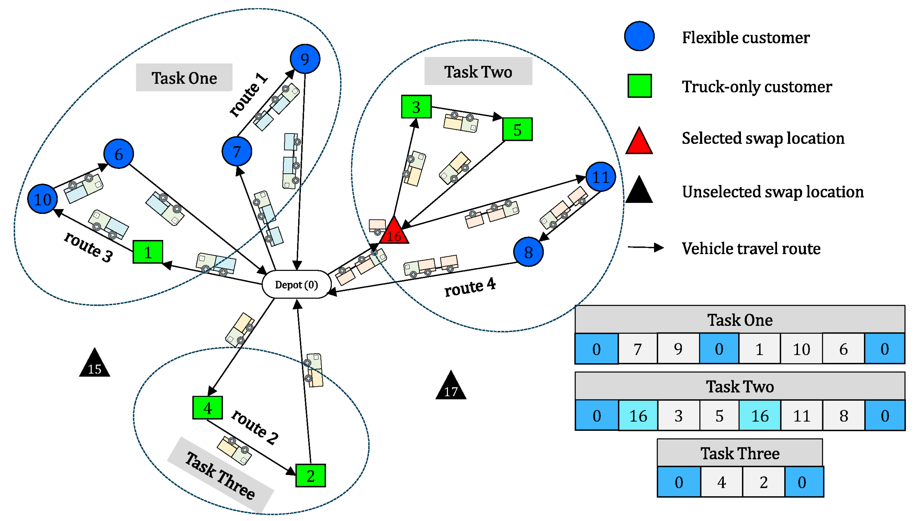
As shown in Figure 2, the example solution includes three tasks. Task one consists of multiple routes (routes 1 and 3). In this solution, there are three vehicles: one truck and two trailers. Task one is completed by the same vehicle, which serves customers on route 1 with a trailer and on route 3 with the truck. Route 4 contains a sub-route, indicating the use of a swap location. At this swap location, the vehicle’s swap-body is temporarily stored while the truck continues to serve two truck-only customers.

2.2. Model Formulation

The objective is to minimize the delivery cost Z , which includes the driver’s wage Z 1 , the use cost of the swap location Z 2 , and the vehicle cost Z 3 . Vehicle cost is further divided into the fixed cost of renting the vehicle Z 3 , the driving cost Z 3 , and the variable fuel cost Z 3 , which differs between trucks and trailers. The driving cost pertains to fuel consumption based on distance, irrespective of the load. Variable fuel cost is calculated based on both distance and load. Various internal and external factors, such as vehicle weight, driver behavior, road conditions, and environmental conditions, can affect fuel consumption [36,37,38,39,40]. The fuel consumption function proposed by Barth et al. [41] is used to calculate variable fuel consumption. When a vehicle with a load Q travels a distance d at a constant speed v , its fuel consumption is calculated as follows.
F = λ k N e P d v + γ β d v 2 + γ α Q 0 + Q d
where λ = 1 / k ψ , γ = 1 / 1000 ε ω , β = 0.5 C d A ρ , α = g sin ϕ + g C r cos ϕ ; all indicate fuel consumption parameters. k denotes the calorific value of the fuel. ψ denotes the weight–volume conversion unit (converted from g/s to L/s). N e denotes engine speed. P denotes engine displacement. ε denotes power trailer efficiency. ω denotes the efficiency parameter of the diesel engine. C d and C r denote constants related to air resistance and rolling resistance, respectively. A denotes the cross-sectional area of the vehicle. ρ denotes the air density. g denotes the gravitational acceleration constant. φ denotes the road surface inclination angle. Q 0 denotes the vehicle equipment quality.
Equation (1) can be divided into three parts: the first part represents engine fuel consumption, the second part accounts for speed-related fuel consumption, and the third part pertains to weight-related fuel consumption, which is directly associated with the vehicle’s weight and the distance traveled. Additionally, the fuel consumption cost is categorized into Z 3 and Z 3 . Therefore, Equation (1) is simplified to Equation (2), which is used to calculate the variable fuel cost. Here, δ is the price of fuel, and Δ is the variable fuel cost per ton kilometer.
Z 3 = δ λ γ α Q d = Δ Q d
All symbols used in the SBVRP-FMT model are defined in Table 1.
The SBVRP-FMT is formulated as follows.
Objective function:
min Z = Z 1 + Z 2 + Z 3
Z 1 = f 0 k K y k
Z 2 = θ k K r R i S j C 1 x i j k , r
Z 3 = f 1 k K y k + f 2 e E y e
Z 3 = ρ 1 k K r R i V j V , j i d i j x i j k , r + ρ 2 e E r R i V j V , j i d i j x i j e , r
Z 3 = Δ k K r R i V j V , j i d i j w i j k , r + e E r R i V j V , j i d i j w i j e , r
Constraints:
k K r R i V , i j x i j k , r = 1 , j V / S k K r R j V , j i x i j k , r = 1 , i V / S
i V , i j x i j k , r = 0   o r   2 , k K ; r R ; j S j V , j i x i j k , r = 0   o r   2 , k K ; r R ; i S
e E i V , i j x i j e , r = 0 , r R ; j C 1 e E j V , j i x i j e , r = 0 , r R ; i C 1
e E i V , i j x i j e , r 1 , r R ; j C 2 e E j V , j i x i j e , r 1 , r R ; i C 2
i V , i j x i j k , r = h V , h j x j h k , r , k K ; r R ; j V i V , i j x i j e , r = h V , h j x j h e , r , e E ; r R ; j V
j V / 0 x 0 j k , r y k , k K ; r R j V / 0 x 0 j e , r y e , e E ; r R
k K x i j k , r = 1 , e E x i j e , r 1 , r R ; i , j C 2 , j i
i V / 0 w i , 0 k , r = 0 , k K ; r R i V / 0 w i , 0 e , r = 0 , e E ; r R
j V w j , i k , r = j V w i , j k , r + q i , k K ; r R ; i , j A j V w j , i e , r = j V w i , j e , r + q i , e E ; r R ; i , j A
i C 1 C 2 j C 1 C 2 , j i q i x i j k , r 2 Q max i C 1 C 2 j C 1 C 2 , j i q i x i j k , r e E i C 1 C 2 j C 1 C 2 , j i q i x i j k , r Q max k K ; r R
r R i V j V d i j x i j k , r D max , k K
Equation (9) ensures that each customer node on the road network, excluding swap locations, is served by exactly one truck route and is visited only once. Equation (10) restricts routes that allow drop and pull transport to only one trailer drop operation. Equation (11) specifies that no trailer route on the road network passes through a restricted location. Equation (12) limits the maximum number of trailer routes passing through a flexible location to one, or none. Equation (13) enforces a balance constraint for vehicles entering and exiting a node. Equation (14) specifies that a vehicle can depart from the depot at most once per trip. Equation (15) mandates that the value taken by the trailer is no more than one, while the truck must be included in the route. Equation (16) indicates that the vehicle load is zero upon returning to the depot. Equation (17) describes the change in vehicle load when visiting a customer node. Equation (18) sets the vehicle load constraint. Equation (19) restricts the total distance a truck can travel to complete r trips to no more than the maximum distance a driver can travel in a day.

3. Hybrid Multi-Population Genetic Algorithm

The rationale for proposing a hybrid multi-population genetic algorithm (HMGA) with local search is multifaceted. Firstly, local search effectively identifies local optima by exploring different regions of the search space [42]. Secondly, genetic algorithms provide robust global search capabilities. Furthermore, employing a multi-population strategy enhances search efficiency and accelerates the evolutionary process. The framework of the HMGA algorithm is illustrated in Figure 3.

3.1. Coding and Decoding

3.1.1. Coding

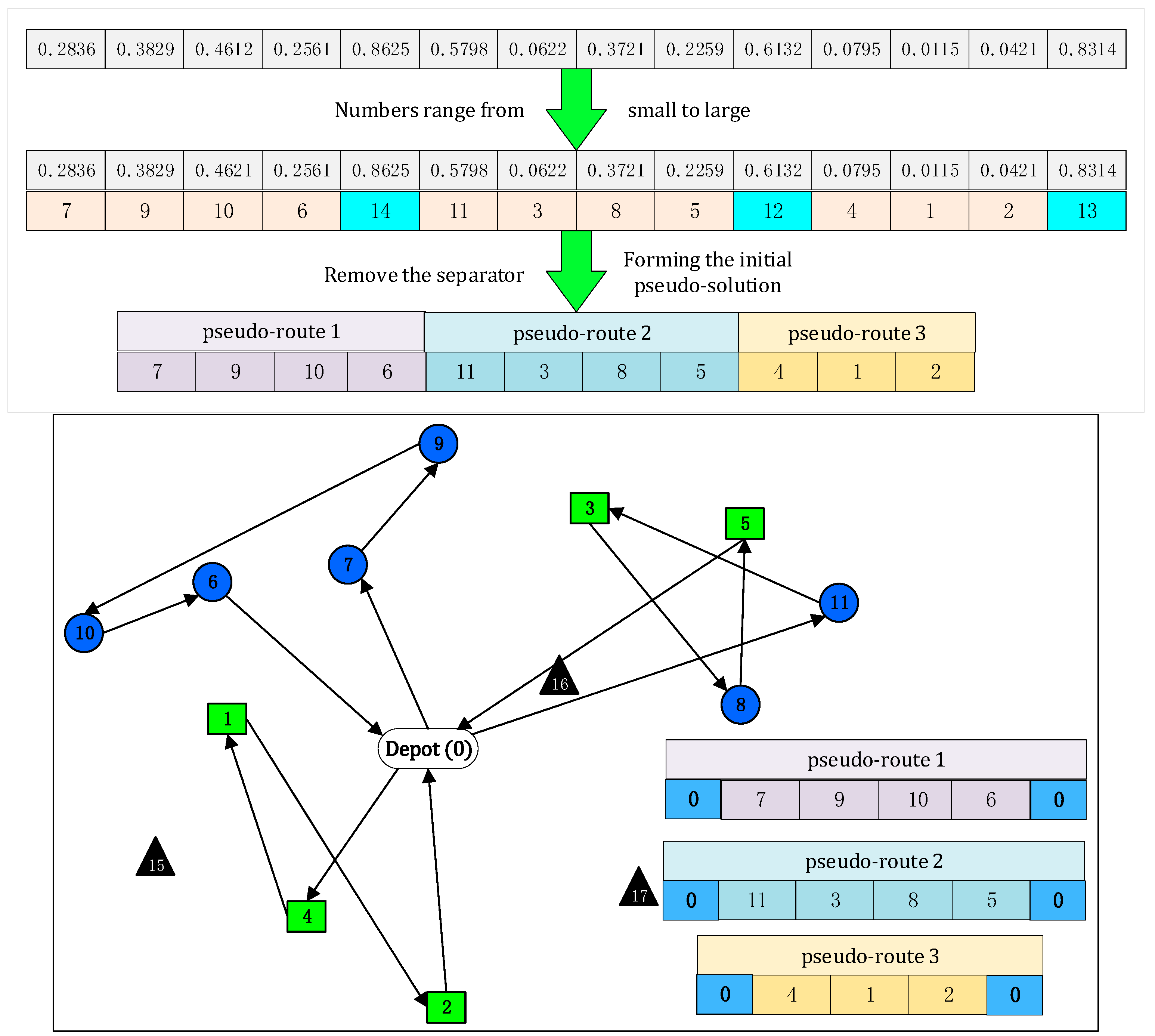
An individual is encoded as a decimal vector. If the number of truck-only customers is n , the number of flexible customers is m , and the number of separators is l , then the length of the individual is n + m + l . There are separators to separate individuals into multiple route segments. For an example depicted in Figure 4, the number of truck-only customers is 5, and the number of flexible customers is 6. If the number of separators is 3, the length of the individual is 14, and an individual can be randomly generated as follows {0.2836, 0.3829, 0.4612, 0.2561, 0.8625, 0.5798, 0.0622, 0.3721, 0.2259, 0.6132, 0.0795, 0.0115, 0.0421, 0.8314}.

3.1.2. Decoding

  • Step 1: Separating individuals into pseudo routes
As illustrated in Figure 4, the example above demonstrates the process of converting an individual into a pseudo route. In this pseudo route, truck-only customer indices range from 1 to 5, flexible customer indices range from 6 to 11, and separator indices range from 12 to 14. The generated random sequence is sorted in ascending order, after which the type of each point is determined based on its position in the sorted sequence. The sequence is then converted into a pseudo-route according to the separators.
  • Step 2: Feasible vehicle loading
The routes obtained from Step 2 may be infeasible if the total demand of a sub-route or route exceeds the loading capacity of the truck or trailer. To address this, Algorithm 1 is employed to ensure the routes are load-feasible. This process consists of two steps: removal and playback operations. The removal operation involves transforming the infeasible solution caused by capacity limitations into a feasible one by removing nodes that exceed the capacity limit. The playback operation then involves adding the removed nodes back into the route to form a new feasible solution. Figure 5 illustrates a solution for the pseudo-routes depicted in Figure 4.
Algorithm 1: Feasible Vehicle Loading
Input: Solution τ , customer demand q , truck loading capacity Q , empty set Ψ , route ξ with no customers.
Output: τ
//Removal operation
for each route τ i τ
    Differentiating truck-only customer set R i and flexible customer set F i from τ i
     Q s u m k R i q k
    while  Q s u m > Q
        Remove one customer from set R i to set Ψ and delete it from τ i
         Q s u m k R i q k
     end
     Q s u m k R i F i q k
    while  Q s u m > 2 Q
        Remove one customer in set F i to set Ψ and delete it from τ i
         Q s u m k R i F i q k
     end
end
//Playback operation
for each customer ψ j Ψ
    if  ψ j C 1
         ϑ 0
        for each τ i τ
             Q s u m k R i q k + q ψ j
            if  Q s u m Q
                 Ψ Ψ \ ψ j ; τ i τ i ψ j
                 ϑ 1
                break
            end
        end
        if  ϑ = 0
             ξ ξ ψ j ; τ τ ξ
         end
    else
         ϑ 0
        for each τ i τ
             Q s u m k R i F i q k + q ψ j
            if  Q s u m 2 Q
                 Ψ Ψ \ ψ j ; τ i τ i ψ j
                 ϑ 1
                break
            end
        end
        if  ϑ = 0
             ξ ξ ψ j ; τ τ ξ
         end
     end
end
  • Step 3: Adding swap locations
This process involves identifying swap routes that require swap locations (swap routes), reordering customers on these swap routes, and separately selecting the swap locations to add onto these routes.
(1) Identifying swap routes
The flow chart in Figure 6 summarizes the method to identify swap routes. Let the total demand for route i be i , that is i = k R i F i q k . Suppose 1 > Q , 2 > Q , 3 Q , and 4 Q in Figure 5. Then pseudo-route 1 can be served by trailer because there are no truck-only customers on this route. Pseudo-routes 3 and 4 can obviously be served by trucks. Because there are truck-only customers on pseudo-route 2 and 2 > Q , this route is a swap route and needs to add a swap location.
(2) Reordering customers on swap routes
The delivery order of customers on each swap route should be adjusted so that truck-only customers are grouped together. For example, in Figure 5, the reordered pseudo-solution is depicted in Figure 7.
(3) Setting swap locations
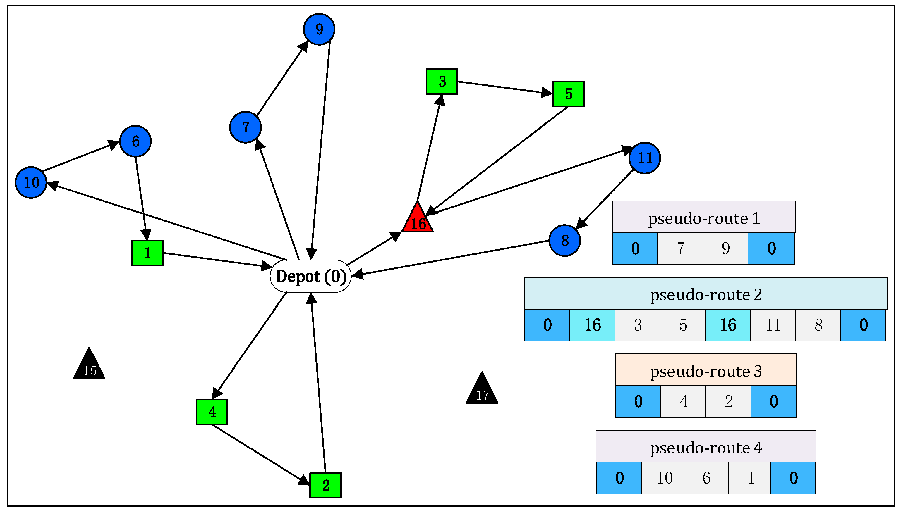
For each swap route, the closest swap location to the first truck-only customer is selected. For example, in pseudo-route 2 shown in Figure 8, swap location 16 is chosen because it is closest to customer 3. The vehicle drives to swap location 16, parks the trailer, and serves the truck-only customers. Once the service for the truck-only customers is complete, the vehicle returns to swap location 16, hitches the trailer, and resumes the delivery route, as illustrated in Figure 8.
  • Step 4: Assigning delivery tasks (trips)
The Next Fit algorithm (see Algorithm 2) is employed to assign routes to vehicles (tasks), where each vehicle is treated as a container. The maximum travel distance allowed for each vehicle, D max , represents the capacity of the container. Figure 2 illustrates a solution based on the pseudo-solution shown in Figure 8.
Algorithm 2: Task Assignment
Input: Solution τ , number of routes n ,   D max , total distance D τ i of τ i τ , number of vehicles h , empty set ( χ j ) and υ ( ν j υ ).
Output:  , υ .
for each route τ i
      ϑ 0
     while  ν j + D τ i D max
    χ j χ j τ i ;   ν j ν j + D τ i
    ϑ 1
    end
    if  ϑ = 0
   χ n e w τ i ;   ν n e w 0
   χ n e w ;   υ υ ν n e w
     end
end

3.2. Genetic Algorithm Operation

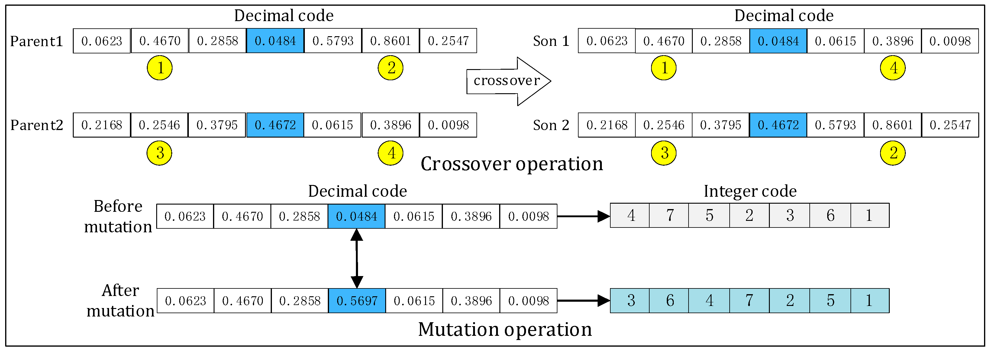
Roulette is used for individual selection. Figure 9 depicts the crossover and mutation operations. The crossover operation involves swapping portions of chromosomes between two selected individuals to create new offspring. As illustrated in Figure 9, a 2-gene segment from Parent 1 is exchanged with a 4-gene segment from Parent 2, resulting in two new offspring. Additionally, the mutation operation is performed by replacing a segment of the chromosome with a randomly generated value. For example, the original decimal “0.0484” is replaced with a new value, “0.5697”, as shown in Figure 9.

3.3. Population Evolution Strategy

Figure 10 illustrates the multi-population evolution strategy (MPES), where a population is divided into multiple subpopulations that evolve independently. The best local solutions from each subpopulation (L-Best) are shared to update the global best solution (G-Best). Additionally, the worst individual from each subpopulation is replaced by the G-Best solution. Notably, Figure 10 shows two different cross-mutation probabilities (pc-pm and PC-PM), which are of significance.

3.4. Local Search

The local search (LS) consists of both sub-route and route-level optimizations. The sub-route local search aims to improve solutions by randomly swapping customer nodes within the sub-route. The route-level local search, on the other hand, attempts to enhance solutions by randomly swapping nodes within the route, treating each sub-route as a single node. Figure 11 provides a schematic diagram illustrating the local search process.

4. Computational Experiments

The proposed HMGA algorithm was implemented in Matlab R2014a and tested on a Windows 10 computer with an Intel Core i7 CPU. Experimental data were generated from the Solomon Benchmark R101. In this dataset, node 1 is designated as the depot, nodes 2–11 as swap locations, nodes 12–61 as flexible nodes, and nodes 62–101 as restricted locations.
Let Q max be 200, the fixed cost of renting a truck and a trailer be 1 and 2, respectively, and the driving cost per distance for a truck and a trailer be 1 and 1.5, respectively. The cost of using a swap location is 5. The driver’s daily wage is 10, D max is 1000, and the variable fuel cost per ton-kilometer is 0.03.
To evaluate the effectiveness of the different components and the overall performance of the proposed method, we conducted experiments by removing each component of the HMGA algorithm in turn. Running the algorithm without a local search (LS) and multi-population evolution strategy (MPES) produced the “GA” version. The “MGA” version was obtained by excluding LS, while the “HGA” version was derived without an MPES.
This section begins with Section 4.1, which analyzes the performance of different algorithmic components. In Section 4.2, different algorithmic versions are analyzed by adjusting the parameters of crossover and mutation operations.

4.1. Performance of Different Algorithmic Versions

Let the population size be 200, with pc and PC both set to 0.9 and pm and PM both set to 0.1. The maximum number of iterations is 50, and the local search to improve individuals is performed 50 times. Each different algorithmic version is run 30 times.
As shown in Figure 12, the average number of iterations (the average iterations when the best solution is first found) for the GA is 38.23, while for the MGA, it is 29.43. This represents a reduction of approximately 23.02% for the MGA compared to the GA. The average running time for the GA is 457.97 s, while for the MGA, it is 239.17 s, reflecting an improvement of about 47.78%. The MGA outperforms the GA in both average iterations and average running time. Similarly, the average number of iterations for the HGA is 31.35, which is about 18.00% lower than that of the GA but about 6.52% higher than that of the MGA. The average running time for the HGA is 323.63 s, showing an improvement of about 29.33% compared to the GA, but it is 84.46 s longer than the MGA. These results demonstrate that the MPES and LS components have a beneficial impact on both average iterations and average running time.
Table 2 presents the average costs for the optimal routes found using the four algorithm versions. The total cost of the best solution identified by the HGA, MGA, and HMGA is reduced by 19.59%, 6.67%, and 21.21%, respectively, compared to the solution generated by the GA. Additionally, when fuel consumption is taken into account, the HMGA achieves a 27.52% reduction in fuel costs compared to the GA. These results demonstrate that enterprises can leverage the proposed method to identify more cost-effective and energy-efficient routes, thereby supporting their development, conserving energy, and reducing carbon emissions.
Figure 13 shows that the results obtained by the HGA are superior and more centralized, with no outliers. Additionally, Figure 14 provides an intuitive comparison between the best solutions of the GA and HMGA. It is evident that the routes obtained by the HMGA are more concise compared to those from the GA. For instance, consider the highlighted red route: the driving distance for the GA is 292.1, while for the HMGA, it is 199.3. This represents a reduction of approximately 31.8%.
By dividing the initial population into multiple sub-populations that evolve independently, the MPES effectively explores the solution space, minimizing the risk of getting trapped in local optima. Periodically, these sub-populations communicate to share their best solutions, updating the global optimal solution by replacing the worst individual in each population. This collaborative evolution drives each sub-population toward better solutions, enhancing solution efficiency. LS, meanwhile, starts with an initial solution and iteratively generates neighborhood solutions, selecting the best one based on solution quality. When combined with the global search strategy of the GA, LS refines the solution with each new population, quickly identifying locally optimal solutions, further boosting solution quality and efficiency. Consequently, the MGA and HGA offer superior solution quality, efficiency, and time performance compared to the GA, while the HMGA, integrating LS and the MPES, delivers an even more efficient solution process with enhanced optimization capability.

4.2. Impacts of Crossover and Mutation Parameters

We want to investigate the impacts of crossover and mutation parameters on the performance of different algorithmic versions. The parameters for the analysis are set as the following: The population size was set to 200, with a maximum of 50 iterations. The local search to improve individuals was performed 50 times. Each different algorithmic version was run 10 times. The results are summarized in Table 3 and Table 4.
Table 3 presents the average values of the different algorithmic versions. The results clearly show that the average value of the HMGA is the smallest under the same parameters. Additionally, the LS component significantly improves the solution of the proposed problem.
In Table 4, B and A denote the best solution costs and average solution costs, respectively. %B and %A represent the percentage deviations of the HMGA from the MGA in terms of B and A, respectively. Table 4 clearly demonstrates that the LS component not only enhances the average solution costs but also improves the best solution costs by approximately 20% under identical parameters. Table 3 and Table 4 collectively indicate that the probabilities of crossover and mutation operations significantly influence the optimization performance of the algorithm.

5. Conclusions

Our proposed swap-body vehicle routing problem with fuel consumption and multiple trips (SBVRP-FMT) extends the existing SBVRP, a variant of the VRP that has been extensively studied and includes quite a few practical complexities. To maintain sustainability, companies must reduce delivery costs, with fuel consumption management and multiple vehicle trips being two effective strategies. This paper integrates these two factors into the SBVRP framework, aiming to minimize total delivery costs through a hybrid multi-population genetic algorithm (HMGA) designed to solve this NP-hard problem. The proposed method was tested on an instance generated from Solomon Benchmark R101 with 101 nodes, including 40 truck-only customers and 50 flexible customers. The experimental results highlight the effectiveness of the algorithm’s components. A comparative analysis reveals that the HMGA algorithm reduces total cost expenses by 21.21% and saves 27.52% on fuel consumption compared to the GA algorithm. This research will have positive implications for the transportation field and delivery industry, ultimately contributing to sustainable development.
A proposed route solution incorporates fuel management and multi-trip scheduling as effective methods for cost reduction. The real-world applicability of this solution could be further validated by incorporating empirical studies in future research. However, there are some limitations to this study. (1) The assumptions are idealized. In reality, road traffic conditions fluctuate over time, but this study assumes a constant average vehicle speed, which is unrealistic. (2) Given the relatively limited impact of road characteristics on fuel consumption compared to route length and load factors, this study focuses solely on fuel consumption related to load and route length while overlooking the influence of road conditions.
Emerging research on real-time traffic path optimization algorithms using big data analytics offers promising opportunities. Traffic data obtained through these techniques can more accurately reflect actual conditions. To address the limitations and better account for road characteristics in fuel consumption, future research could integrate big data analysis to provide a precise foundation for optimizing traffic paths, enhancing both the model’s realism and the algorithm’s accuracy. Additionally, future studies could explore whether the adoption of emerging technologies like electric vehicles could further reduce operating costs and carbon emissions.

Author Contributions

Conceptualization, Y.P. and Y.L.; Methodology, Y.P., Y.Z., D.Z.Y., S.L. and Y.L.; Formal Analysis, D.Z.Y. and Y.L.; Data Curation, Y.P., Y.Z., S.L. and Y.L.; Writing—Original Draft, Y.Z. and S.L.; Writing—Review and Editing, D.Z.Y. and Y.S.; Visualization, D.Z.Y. and Y.S.; Supervision, D.Z.Y.; Project Administration, D.Z.Y.; Funding Acquisition, Y.P. All authors have read and agreed to the published version of the manuscript.

Funding

The research is supported by the Graduate Student Tutor Team Building Program in Chongqing, China No. JDDSTD2022004, Graduate Student Research Innovation Program of Chongqing Jiaotong University No. 2023S0060, and Communications Science and Technology Project in Chongqing, China No. CQJT-2024CZ28-3 and No. CQJT-2024CZ31-1.

Institutional Review Board Statement

Not applicable.

Informed Consent Statement

Not applicable.

Data Availability Statement

The data are available upon request.

Conflicts of Interest

Yuanjun Li was employed by the Chongqing Jiangjin District Road Transportation Affairs Center. The remaining authors declare that the research was conducted in the absence of any commercial or financial relationships that could be construed as a potential conflict of interest.

References

  1. Lehmann, J.; Winkenbach, M. A matheuristic for the two-echelon multi-trip vehicle routing problem with mixed pickup and delivery demand and time windows. Transp. Res. Part C Emerg. Technol. 2024, 160, 104522. [Google Scholar] [CrossRef]
  2. Yaiprasert, C.; Hidayanto, A.N. AI-powered ensemble machine learning to optimize cost strategies in logistics business. Int. J. Inf. Manag. Data Insights 2024, 4, 100209. [Google Scholar] [CrossRef]
  3. Luo, R.; Ji, S.; Ji, T. An effective chaos-driven differential evolution for multi-objective unbalanced transportation problem considering fuel consumption. Appl. Soft Comput. 2021, 101, 107058. [Google Scholar] [CrossRef]
  4. Gkyrtis, K. Theoretical considerations from the modelling of the interaction between road design and fuel consumption on urban and suburban roadways. Modelling 2024, 5, 737–751. [Google Scholar] [CrossRef]
  5. Liu, J.; Feng, L.; Li, Z. The Optimal Road Grade Design for Minimizing Ground Vehicle Energy Consumption. Energies 2017, 10, 700. [Google Scholar] [CrossRef]
  6. Heid, W.; Hasle, G.; Vigo, D. Verolog solver challenge 2014–VSC2014 problem description. In VeRoLog; (EURO Working Group on Vehicle Routing and Logistics Optimization) and PTV Group, 2014; pp. 1–6. Available online: https://verolog.euro-online.org/wp-content/uploads/2021/09/CallVeRoLogChallenge2014.wh_-2.pdf (accessed on 18 May 2024).
  7. Cordeau, J.F.; Laporte, G.; Savelsbergh, M.W.; Vigo, D. Vehicle routing. In Handbooks in Operations Research and Management Science; Elsevier: Amsterdam, The Netherlands, 2007; Volume 14, pp. 367–428. [Google Scholar]
  8. Huber, S.; Geiger, M.J. Swap body vehicle routing problem: A heuristic solution approach. In Proceedings of the Computational Logistics: 5th International Conference, ICCL 2014, Valparaiso, Chile, 24–26 September 2014; Springer International Publishing: Cham, Switzerland, 2014; pp. 16–30. [Google Scholar]
  9. Huber, S.; Geiger, M.J. Order matters–a variable neighborhood search for the swap-body vehicle routing problem. Eur. J. Oper. Res. 2017, 263, 419–445. [Google Scholar] [CrossRef]
  10. Lum, O.; Chen, P.; Wang, X.; Golden, B.; Wasil, E. A heuristic approach for the swap-body vehicle routing problem. In Proceedings of the 14th INFORMS Computing Society Conference, Richmond, VA, USA, 11–13 January 2015; Volume 11, pp. 172–187. [Google Scholar]
  11. Miranda-Bront, J.J.; Curcio, B.; Méndez-Díaz, I.; Montero, A.; Pousa, F.; Zabala, P. A cluster-first route-second approach for the swap body vehicle routing problem. Ann. Oper. Res. 2017, 253, 935–956. [Google Scholar] [CrossRef]
  12. Absi, N.; Cattaruzza, D.; Feillet, D.; Housseman, S. A relax-and-repair heuristic for the Swap-Body Vehicle Routing Problem. Ann. Oper. Res. 2017, 253, 957–978. [Google Scholar] [CrossRef]
  13. Todosijević, R.; Hanafi, S.; Urošević, D.; Jarboui, B.; Gendron, B. A general variable neighborhood search for the swap-body vehicle routing problem. Comput. Oper. Res. 2017, 78, 468–479. [Google Scholar] [CrossRef]
  14. Toffolo, T.A.; Christiaens, J.; Van Malderen, S.; Wauters, T.; Berghe, G.V. Stochastic local search with learning automaton for the swap-body vehicle routing problem. Comput. Oper. Res. 2018, 89, 68–81. [Google Scholar] [CrossRef]
  15. Huber, S.; Cordeau, J.F.; Geiger, M.J. A matheuristic for the swap body vehicle routing problem. OR Spectr. 2020, 42, 111–160. [Google Scholar] [CrossRef]
  16. Karnaukhov, O.; Karnaukhova, I.; Karnaukhov, V.; Ryndina, O. Reducing fuel consumption by using correcting parameters system for heavy duty vehicles. Transp. Res. Procedia 2022, 63, 2820–2828. [Google Scholar] [CrossRef]
  17. Kuo, Y. Using simulated annealing to minimize fuel consumption for the time-dependent vehicle routing problem. Comput. Ind. Eng. 2010, 59, 157–165. [Google Scholar] [CrossRef]
  18. Xiao, Y.; Zhao, Q.; Kaku, I.; Xu, Y. Development of a fuel consumption optimization model for the capacitated vehicle routing problem. Comput. Oper. Res. 2012, 39, 1419–1431. [Google Scholar] [CrossRef]
  19. Pradenas, L.; Oportus, B.; Parada, V. Mitigation of greenhouse gas emissions in vehicle routing problems with backhauling. Expert Syst. Appl. 2013, 40, 2985–2991. [Google Scholar] [CrossRef]
  20. Lin, C.; Choy, K.L.; Ho, G.T.; Chung, S.H.; Lam, H.Y. Survey of green vehicle routing problem: Past and future trends. Expert Syst. Appl. 2014, 41, 1118–1138. [Google Scholar] [CrossRef]
  21. Alinaghian, M.; Naderipour, M. A novel comprehensive macroscopic model for time-dependent vehicle routing problem with multi-alternative graph to reduce fuel consumption: A case study. Comput. Ind. Eng. 2016, 99, 210–222. [Google Scholar] [CrossRef]
  22. Liu, C.; Kou, G.; Zhou, X.; Peng, Y.; Sheng, H.; Alsaadi, F.E. Time-dependent vehicle routing problem with time windows of city logistics with a congestion avoidance approach. Knowl. -Based Syst. 2020, 188, 104813. [Google Scholar] [CrossRef]
  23. Utama, D.M.; Yurifah, A.; Garside, A.K. A novel hybrid spotted hyena optimizer: An algorithm for fuel consumption capacitated vehicle routing problem. Int. J. Technol. 2023, 14, 1049–1059. [Google Scholar] [CrossRef]
  24. Rahul, J.K.; Chakraborty, S.; Khayer, N.; Uddin, M.F.; Haque, M.R. Designing an Energy-Efficient Transportation Network to Transport Perishable Crops: An Aggregated VRP and X-means Clustering Approach. Heliyon 2023, 9, e19692. [Google Scholar] [CrossRef]
  25. Fernando, W.M.; Thibbotuwawa, A.; Perera, H.N.; Nielsen, P.; Kilic, D.K. An integrated vehicle routing model to optimize agricultural products distribution in retail chains. Clean. Logist. Supply Chain. 2024, 10, 100137. [Google Scholar] [CrossRef]
  26. Pak, Y.J.; Mun, K.H. A practical vehicle routing problem in small and medium cities for fuel consumption minimization. Clean. Logist. Supply Chain. 2024, 100164. [Google Scholar] [CrossRef]
  27. Brandão, J.C.S.; Mercer, A. The multi-trip vehicle routing problem. J. Oper. Res. Soc. 1998, 49, 799–805. [Google Scholar] [CrossRef]
  28. Fleischmann, B. The Vehicle Routing Problem with Multiple Use of Vehicles; Fachbereich Wirtschaftswissenschaften, Universität Hamburg: Hamburg, Germany, 1990. [Google Scholar]
  29. Tirkolaee, E.B.; Hosseinabadi, A.A.R.; Soltani, M.; Sangaiah, A.K.; Wang, J. A hybrid genetic algorithm for multi-trip green capacitated arc routing problem in the scope of urban services. Sustainability 2018, 10, 1366. [Google Scholar] [CrossRef]
  30. Pan, B.; Zhang, Z.; Lim, A. Multi-trip time-dependent vehicle routing problem with time windows. Eur. J. Oper. Res. 2021, 291, 218–231. [Google Scholar] [CrossRef]
  31. Şahin, M.K.; Yaman, H. A branch and price algorithm for the heterogeneous fleet multi-depot multi-trip vehicle routing problem with time windows. Transp. Sci. 2022, 56, 1636–1657. [Google Scholar] [CrossRef]
  32. Pham, Q.D.; Nguyen, T.H.; Bui, Q.T. Modeling and solving a multi-trip multi-distribution center vehicle routing problem with lower-bound capacity constraints. Comput. Ind. Eng. 2022, 172, 108597. [Google Scholar]
  33. Sugianto, W.C.; Kim, B.S. Iterated variable neighborhood search for integrated scheduling of additive manufacturing and multi-trip vehicle routing problem. Comput. Oper. Res. 2024, 167, 106659. [Google Scholar] [CrossRef]
  34. Calamoneri, T.; Corò, F.; Mancini, S. Management of a post-disaster emergency scenario through unmanned aerial vehicles: Multi-Depot Multi-Trip Vehicle Routing with Total Completion Time Minimization. Expert Syst. Appl. 2024, 251, 123766. [Google Scholar] [CrossRef]
  35. Zhao, J.; Poon, M.; Tan, V.Y.; Zhang, Z. A hybrid genetic search and dynamic programming-based split algorithm for the multi-trip time-dependent vehicle routing problem. Eur. J. Oper. Res. 2024, 317, 921–935. [Google Scholar] [CrossRef]
  36. Boriboonsomsin, K.; Barth, M. Impacts of road grade on fuel consumption and carbon dioxide emissions evidenced by use of advanced navigation systems. Transp. Res. Rec. 2009, 2139, 21–30. [Google Scholar] [CrossRef]
  37. Rahman, S.A.; Masjuki, H.H.; Kalam, M.A.; Abedin, M.J.; Sanjid, A.; Sajjad, H.J.E.C. Impact of idling on fuel consumption and exhaust emissions and available idle-reduction technologies for diesel vehicles—A review. Energy Convers. Manag. 2013, 74, 171–182. [Google Scholar] [CrossRef]
  38. Boriboonsomsin, K.; Durbin, T.; Scora, G.; Johnson, K.; Sandez, D.; Vu, A.; Jiang, Y.; Burnette, A.; Yoon, S.; Collins, J.; et al. Real-world exhaust temperature profiles of on-road heavy-duty diesel vehicles equipped with selective catalytic reduction. Sci. Total Environ. 2018, 634, 909–921. [Google Scholar] [CrossRef]
  39. Zhou, M.; Jin, H.; Wang, W. A review of vehicle fuel consumption models to evaluate eco-driving and eco-routing. Transp. Res. Part D Transp. Environ. 2016, 49, 203–218. [Google Scholar] [CrossRef]
  40. Fan, P.; Yin, H.; Lu, H.; Wu, Y.; Zhai, Z.; Yu, L.; Song, G. Which factor contributes more to the fuel consumption gap between in-laboratory vs. real-world driving conditions? An independent component analysis. Energy Policy 2023, 182, 113739. [Google Scholar] [CrossRef]
  41. Barth, M.; Younglove, T.; Scora, G. Development of a Heavy-Duty Diesel Modal Emissions and Fuel Consumption Model; Institute of Transportation Studies, UC Berkeley: Berkeley, CA, USA, 2005. [Google Scholar]
  42. Derbel, H.; Jarboui, B.; Hanafi, S.; Chabchoub, H. Genetic algorithm with iterated local search for solving a location-routing problem. Expert Syst. Appl. 2012, 39, 2865–2871. [Google Scholar] [CrossRef]
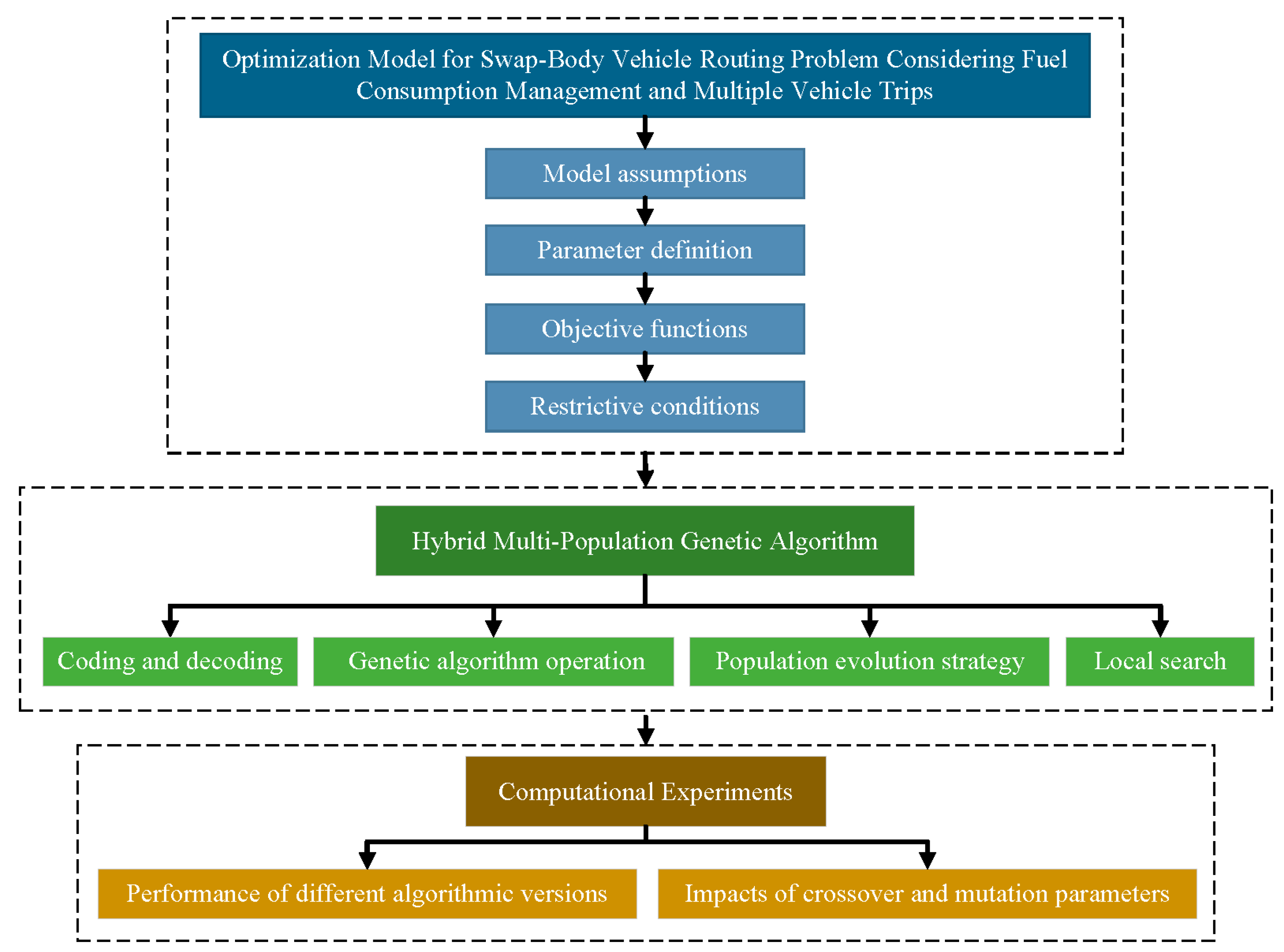
Figure 1. Framework of SBVRP-FMT optimization.
Futuretransp 04 00048 g001
Figure 2. An example solution of the SBVRP-FMT.
Futuretransp 04 00048 g002
Figure 3. The framework of the HMGA.
Futuretransp 04 00048 g003
Figure 4. Pseudo-routes are obtained by separating individuals.
Futuretransp 04 00048 g004
Figure 5. Pseudo-routes with feasible vehicle loading.
Futuretransp 04 00048 g005
Figure 6. Process of identifying swap routes.
Futuretransp 04 00048 g006
Figure 7. Reordering customers on swap routes.
Futuretransp 04 00048 g007
Figure 8. Pseudo-solution after setting swap locations.
Futuretransp 04 00048 g008
Figure 9. Crossover and mutation operations.
Futuretransp 04 00048 g009
Figure 10. Multi-population evolution strategy.
Futuretransp 04 00048 g010
Figure 11. Schematic diagram of local search.
Futuretransp 04 00048 g011
Figure 12. Average iterations and running time of different algorithmic versions.
Futuretransp 04 00048 g012
Figure 13. Solution values of different algorithmic versions.
Futuretransp 04 00048 g013
Figure 14. Best solutions of GA and HMGA.
Futuretransp 04 00048 g014
Table 1. Symbolic definition for the SBVRP-FMT.
SymbolDefinition
Sets
C 1 Set of customers delivered by truck only, C 1 = 1 , 2 , , c 1
C 2 Set of customers that can be delivered by truck or trailer, C 2 = c 1 + 1 , c 1 + 2 , , c 1 + c 2
S Set of swap locations, S = c 1 + c 2 + 1 , c 1 + c 2 + 2 , , c 1 + c 2 + s
V Set of all nodes, V = C 1 C 2 S 0
K Set of trucks, K = 1 , 2 , , k
E Set of trailers, E = 1 , 2 , , e
R Set of trips, R = 1 , 2 , , r
A Set of all arcs, A = i , j | i , j V
Parameters
d i j Distance traveled by the truck from node i to node j
q i Demand for node i
θ Use costs of swap location
f 0 Salary of driver
f 1 , f 2 Fixed cost of renting a truck or trailer
ρ 1 , ρ 2 Driving cost per distance of truck or trailer
Δ Variable fuel cost per ton-kilometer
D max Maximum distance allowed for drivers to work per day
Q max Rated load capacity of trucks or trailer
Decision Variables
x i j k , r The value is 1 if there is a direct route through arc i , j and it belongs to the r -th trip of truck k , otherwise 0, i , j N , k K , r R
x i j e , r The value is 1 if there is a direct route through arc i , j and it belongs to the r -th trip of trailer e , otherwise 0, i , j N , e E , r R
y k The value is 1 if truck k is selected, otherwise 0
y e The value is 1 if trailer e is selected, otherwise 0
w i j k , r The load of truck k when it travels arc i , j at its r -th trip
w i j e , r The load of trailer e when it travels arc i , j at its r -th trip
Table 2. Cost comparison of different algorithmic versions.
Algorithmic VersionsTotal CostsFuel ConsumptionProportion of Total Cost ReductionPercentage of Fuel Cost Reduction
GA66613565
HGA5356264819.59%25.72%
MGA621731826.67%10.74%
HMGA5248258421.21%27.52%
Table 3. Results of different algorithmic versions.
pc–pmGAHGAMGA (PC = 0.9, PM = 0.1)HMGA (PC = 0.9, PM = 0.1)PC-PMMGA (pc = 0.9, pm = 0.1)HMGA (pc = 0.9, pm = 0.1)
0.5–0.165005352648453030.5–0.160055195
0.5–0.265115498667154140.5–0.267025796
0.5–0.366865467656552360.5–0.365305499
0.5–0.466025338655553050.5–0.463345291
0.5–0.564635141627651210.5–0.563525218
0.6–0.169975712671154420.6–0.167215589
0.6–0.265935304689852250.6–0.262115303
0.6–0.369625670652952620.6–0.366545926
0.6–0.468345792680756770.6–0.463405313
0.6–0.568265483663053650.6–0.564365530
0.7–0.166385380676853760.7–0.163785053
0.7–0.269055442679752790.7–0.264055427
0.7–0.365635375656851420.7–0.367785497
0.7–0.468775885707055790.7–0.467445596
0.7–0.569675775640651550.7–0.564075405
0.8–0.166295579653650510.8–0.165375543
0.8–0.268545168614849920.8–0.266235536
0.8–0.368675613681653580.8–0.366135360
0.8–0.466325547633254390.8–0.463555238
0.8–0.566785708699260850.8–0.565795533
0.9–0.168365059649350690.9–0.163055194
0.9–0.265305324684551920.9–0.258785128
0.9–0.365725407680251880.9–0.362795222
0.9–0.464235555660454780.9–0.465275520
0.9–0.568185475670053200.9–0.565315671
Table 4. Best solution costs, average solution costs, and corresponding deviations of MGA and HMGA.
pc–pmPC–PMMGAHMGA
BABA%B%A
0.5–0.10.9–0.16258654852975471−15.36−16.45
0.9–0.10.5–0.16524681252435492−19.64−19.38
0.5–0.20.9–0.16518664551405409−21.14−18.6
0.9–0.10.5–0.26415679954145618−15.6−17.37
0.5–0.30.9–0.16160651550925338−17.34−18.07
0.9–0.10.5–0.36345673348675467−23.29−18.8
0.5–0.40.9–0.16609666549985428−24.38−18.56
0.9–0.10.5–0.46157641448475207−21.28−18.82
0.5–0.50.9–0.16277642249595134−21−20.06
0.9–0.10.5–0.56179638249295381−20.23−15.68
0.6–0.10.9–0.15914659549695480−15.98−16.91
0.9–0.10.6–0.16597681753205573−19.36−18.25
0.6–0.20.9–0.16718698554485774−18.9−17.34
0.9–0.10.6–0.26228664551165492−17.85−17.35
0.6–0.30.9–0.16538674049245415−24.69−19.66
0.9–0.10.6–0.36666681753215504−20.18−19.26
0.6–0.40.9–0.16495673550965472−21.54−18.75
0.9–0.10.6–0.46286649553565520−14.79−15.01
0.6–0.50.9–0.16352676451995368−18.15−20.64
0.9–0.10.6–0.56552677750655605−22.7−17.29
0.7–0.10.9–0.16562683951275397−21.87−21.08
0.9–0.10.7–0.16381665551485499−19.32−17.37
0.7–0.20.9–0.16431666551685325−19.64−20.11
0.9–0.10.7–0.26499659151275325−21.11−19.21
0.7–0.30.9–0.16263665350145298−19.94−20.37
0.9–0.10.7–0.36396645754715641−14.46−12.64
0.7–0.40.9–0.16469683351135365−20.96−21.48
0.9–0.10.7–0.46152675151655422−16.04−19.69
0.7–0.50.9–0.16202651451975330−16.2−18.18
0.9–0.10.7–0.56284650554665740−13.02−11.76
0.8–0.10.9–0.16393649050195174−21.49−20.28
0.9–0.10.8–0.16370657352825477−17.08−16.67
0.8–0.20.9–0.15920630550135296−15.32−16
0.9–0.10.8–0.26471660251035320−21.14−19.42
0.8–0.30.9–0.16358653651265463−19.38−16.42
0.9–0.10.8–0.36208643951325555−17.33−13.73
0.8–0.40.9–0.16173667549535338−19.76−20.03
0.9–0.10.8–0.46526681952865595−19−17.95
0.8–0.50.9–0.16371675849815591−21.82−17.27
0.9–0.10.8–0.56391676752935506−17.18−18.63
0.9–0.10.9–0.16194660447305084−23.64−23.02
0.9–0.10.9–0.16306654449145294−22.07−19.1
0.9–0.20.9–0.16187678948065117−22.32−24.63
0.9–0.10.9–0.26413663647135103−26.51−23.1
0.9–0.30.9–0.16759697550675171−25.03−25.86
0.9–0.10.9–0.36587682348025229−27.1−23.36
0.9–0.40.9–0.16195662648295380−22.05−18.8
0.9–0.10.9–0.46353681650575354−20.4−21.45
0.9–0.50.9–0.16114682649375226−19.25−23.44
0.9–0.10.9–0.56341661450735452−20−17.57
Disclaimer/Publisher’s Note: The statements, opinions and data contained in all publications are solely those of the individual author(s) and contributor(s) and not of MDPI and/or the editor(s). MDPI and/or the editor(s) disclaim responsibility for any injury to people or property resulting from any ideas, methods, instructions or products referred to in the content.