Abstract
This paper is concerned with inconsistent results that can be obtained when modeling rigid body collisions via algebraic equations. Newton’s approach is kinematic and fails in several cases. Poisson’s formulation has been shown lead to energetic inconsistencies, particularly in work done by the impulsive forces. This paper shows that the energetic formulation may lead to unexpected results in the magnitudes of the impulsive forces. These inconsistencies are due to the simplifying assumptions made to model collisions as occurring instantaneously. The inconsistencies increase as friction in the system becomes higher. We propose an optimization procedure for solving the algebraic equations of impact so that inconsistencies are minimized. Using experimental results, we present a discussion about the coefficients of restitution and friction.
1. Introduction
Consider an object colliding with another object or with a fixed surface. We observe a few physical phenomena: there is less energy in the object and lower velocities are observed after impact, and the impulsive forces that act during restitution are lower in magnitude than their counterparts during compression. These phenomena have been observed experimentally as well as deduced intuitively. Impact models have been proposed based on these phenomena. At the simplest level, impact modeling by algebraic equations relies on two parameters: the coefficients of restitution and friction [1].
Analyses of friction and impact are centuries old. Leonardo da Vinci’s contributions are described in [2]. Routh [3] developed graphical techniques for modeling impact. The Newton and Poisson models for restitution were the initial widely-used models. The Newton model relates velocities of the impact point before and after impact and the Poisson model relates the impact forces during compression and restitution. The Newton model, which is a kinematic relationship, is widely used in experimental research involving point or small masses, as well as for identifying the coefficient of restitution, e.g., [4,5].
The currently used algebraic equations for rigid body impact in the presence of friction were developed over 30 years ago [6]. These equations were initially used with the Poisson or Newtonian formulations. These two restitution models lead to energetically inconsistent results [7] for modeling rigid body impact. For certain orientations of the body, work done by the restitution force and energy dissipation deviates from expected values. This inconsistency gets worse as the amount of friction in the system increases.
The energetic formulation [7] for the coefficient of friction was developed in response to this inconsistency. Here, the coefficient of restitution is defined as the square root of the ratio of the work done by the restitution force divided by the work done.
A review of the evolution of dynamics of impact can be found in [8], where contact models are analyzed. The Poisson and energetic models give identical results in the absence of friction [9].
The energetic model for restitution leads to energetically consistent results. However, it does not consider the ratio of the normal forces during compression and restitution. We would expect this ratio to follow a similar pattern observed in experiments and in the Poisson model. The question arises as to whether it is possible to use the energetic formulation and have unexpectedly high or low values for the impact forces. A restitution force close in magnitude to the compressive force is an indication of inconsistency. Calculating the force ratio in the energetic formulation was first considered in [10].
This paper builds on the observations in [10] and it analyzes and simulates impact equations. It then compares the work done by the normal force, as well as ratios of the magnitudes of the impulsive forces and points to inconsistencies in the formulation. The analysis assumes that the coefficients of friction and restitution remain constant during impact. The results confirm that the Poisson model may lead to inconsistent results for energy. However, the results also indicate that the energetic approach may produce inconsistent results for force magnitudes. Hence, neither the Poisson, Newton, nor energetic formulations are accurate descriptions of rigid body impact in the presence of friction. This inconsistency is exacerbated for higher values of friction.
What can be done to improve the impact model? To this end, this paper proposes an optimization technique that combines the Poisson and energetic formulations. The paper ends with a discussion and some thoughts about the coefficients of friction and restitution based on experimental results of the author [11].
2. Review of Two-Dimensional Impact Equations
Consider a rigid body of mass m and centroidal moment of inertia impacting a surface. The orientation is shown in Figure 1, where C is the impact point. The body does not need to be a slender rod. We use a fixed set of axes, with the y axis perpendicular to the plane of impact and pointing downward.
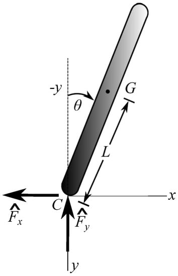
Figure 1.
Free body diagram of 2D model during impact assuming for .
The orientation of the object is defined by the angle . The position vector is
in which L is the distance from the center of mass G to C. The velocity of the center of mass and angular velocity immediately before impact are The impact point velocity at the beginning of impact is .
An impulsive normal force acts in the vertical direction (upwards) and impulsive friction force opposite to the horizontal velocity of the impact point C. The gravitational force is negligible as it is non-impulsive. We express the total impulsive force as
in which . Assuming that impact takes place in a very short period of time, the linear and angular impulse-momentum relationships can be written as
where the primes denote post-impact quantities. With this notation, and are both positive quantities.
The three equations above are accompanied by five unknowns: three post-impact velocities , , and two impulsive forces , . Two additional equations are needed which are obtained depending on the type of motion and stage of impact.
In each stage of impact, the impact point can undergo four types of motion: (i) it can continue sliding, (ii) sliding can come to a stop and the impact point sticks, (iii) after coming to a stop the impact point begins to slide in the opposite direction (reverse sliding), or (iv) if initial horizontal velocity of impact point is zero, it can continue sticking or begin sliding. Reverse sliding occurs when the moment generated by the impulsive normal force is large enough to reverse the direction of sliding.
Consider the compression stage and where sliding continues throughout. The vertical velocity of the impact point is zero at the end of compression, so that the fourth and fifth equations become
When sliding ends during compression, we split the compression stage into two periods and . The horizontal velocity of the impact point becomes zero before the vertical velocity does. We replace c with , as described in [10].
There are two possibilities during the second part of compression: the impact point sticks or it slides in the opposite direction. We calculate by analyzing the slide direction in the absence of friction. This tendency is dictated by . When , the impact point will slide in the direction and vice versa. The end conditions for sticking are
When reverse sliding occurs, the end conditions are , and , as direction of the friction force has changed. The motions when the initial horizontal velocity is zero, , are described in [10].
We next consider restitution. Here, the impulsive normal force has a smaller magnitude than during compression, primarily due to hysteresis. This loss is modeled by the coefficient of restitution and is denoted by . We begin with the case where at the end of compression the impact point slides and sliding continues during restitution. The three momentum balances are the same as Equation (3) with superscript r. The fourth equation depends on the sliding condition.
When sliding ends during restitution, we separate the restitution stage into two periods, and , and follow a procedure similar to compression [10]. The horizontal velocity of the impact point becomes zero at .
For sticking, the fourth equation is . For reverse sliding, the fourth equation is . As in the compression stage, we calculate friction needed to prevent sliding and compare to the available friction.
The fifth equation in all cases is in terms of the coefficient of restitution . We consider three definitions for . The first definition relates the impulsive normal forces by
and it is attributed to Poisson. The second definition, known as Newton’s law, can be derived from Poisson’s model for simple cases of impact and relates the velocities of the impact point by .
The energetic formulation is in terms of work done by the normal force during the compression and restitution stages. Denoting them by and , the energetic coefficient of restitution is defined as
Work can be defined as the integral of power, that is, force times velocity. For the normal force , . Details of the work expressions can be found in [10]. Work done by the impact force during restitution has a similar form. Seven different cases can be identified for two-dimensional impact, as listed in Table 1. As shown in [10], we can obtain the mode of motion in closed form.

Table 1.
Cases for two-dimensional (also three-dimensional) impact.
3. Non-Dimensional Restitution Parameters and Simulation
The three definitions for coefficient of restitution in the previous section lead to three non-dimensional and normalized quantities
with the subscripts denoting Poisson, Newton, and energetic, respectively. In the absence of friction, all three definitions of the coefficient of restitution are equivalent [7].
We next obtain numerical results by varying the orientation angle and ratio for and . The initial angular velocity is taken as zero. The falling object is a rod with . The plots are given for . These values are chosen so that all modes of motion will be present in the plots [10].
Figure 2 and Figure 3 in [10] show the mode of impact, velocity ratios, total energy ratios, and . We reproduce here the plot of for the Poisson model and for the energetic model. For the Poisson model, plot of shows places where the model produces energetically inconsistent or unreliable results. If the work-done ratio is over 1, then the impulsive normal force increases energy, which is not possible. For the energetic model, plot of shows the ratio of the impulsive forces, and where the energetic model produces unexpected results. For example, indicates that restitution force is larger than the compression force, which is impossible. We make the following observations from the simulation results:
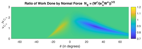
Figure 2.
Influence of orientation angle and velocity ratio for , , on ratio of work done by normal force . Poisson’s model is used.
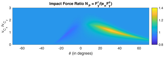
Figure 3.
Influence of orientation angle and velocity ratio for ratio of normal force for restitution and compression . Energetic model is used.
- As discussed in [10], both models produce the same results for the mode of motion. Furthermore, both models produce similar results for the velocity ratio of the impact point, and very similar results for the ratio of total energy.
- The ratio of work done for Poisson’s model in Figure 2 shows an energetic inconsistency for some cases when , with the restitution force doing more work than times than the work done by the compressive forces, while the work done by the restitution force is still less than work done by the compressive force, this ratio is high and unexpected. Furthermore, for certain values when , the restitution force does much less work than expected.
- The ratio of the normal forces in Figure 3, which uses the energetic model for restitution, is quite high in a few cases. There are points on the plot with a force ratio of . The restitution force reaches values of , which is quite high, unexpected, and inconsistent.
- For cases when is larger than one, is less than one and vice versa.
Both plots above point to a band that rises as the orientation angle approaches zero and falls as increases. This band corresponds to regions when sliding ends and the object sticks or reverse slides: in cases 1 and 2 sliding ends during compression and in cases 3 and 4 sliding ends during restitution. This is an indication that sliding coming to an end is not being modeled accurately. Outside of this band, the three normalized quantities have near-identical values, all very close to 1.
As discussed earlier, for zero friction all models give the same results. The Poisson and energetic models begin to diverge as the amount of friction increases, with values deviating more from unity in the Poisson model and values in the energetic model. Furthermore, the Newton model for restitution diverges faster than the Poisson and energetic models.
For a high-friction case, such as , in a few orientations of the object the energetic approach, the impulsive restitution force has a higher magnitude than the impulsive compression force, which is an impossibility. The highest value of for the energetic model is 1.49, so that . The lowest value of is 0.78, which leads to a very small value for the restitution force , which also is not very likely. Furthermore, the band where the values of and deviate from unity becomes thicker with increasing friction.
Similarly, for the Poisson model with , the highest value of is 1.27, so that , which is quite high and unexpected. The lowest value of is 0.67, so that , also not expected.
We should keep in mind that the friction force becomes a greater factor when the horizontal speed is within a certain range. From Figure 2 and Figure 3, for low horizontal to vertical velocity ratios (in our example, ) and high velocity ratios (in our example, ) increase in friction does not affect and as much.
The normalized response characteristics do not change when the coefficient of restitution is varied. Table 2, lists the minimum and maximum values of for the Poisson model and of for the energetic model for different values of and . When is kept the same and is varied, values for and do not change for both the Poisson and energetic models. However, when is kept the same and is varied, there is a substantial difference in the results.
Table 2.
Minimum and maximum values for and for different values of and .
4. Review of Three Dimensional Impact and Simulation
The three-dimensional impact equations have received more interest in recent years, e.g., [12,13,14]. We use here the formulation described in detail in [10]. The derivations are quite lengthy, so that they will only be summarized here. We use the same coordinate system as before. The plane is the plane of impact. The position vector from the center of mass to the impact point is shown in Figure 4.
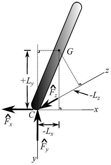
Figure 4.
Falling object colliding with ground in three dimensions.
We express the position vector as
with , where L is the distance from the center of mass G to impact point C.
The initial velocity of the center of mass and angular velocity are , The impact point velocity at the beginning of impact is
Figure 4 also illustrates the impulsive forces acting at the impact point. Defining the magnitudes of these forces as positive, the impulsive force vector becomes
where . The linear momentum balances in the fixed and z-directions are
The angular momentum of a rigid body about its center of mass is , in which is the inertia matrix and is the angular velocity. The angular momentum balance, using a set of body-fixed coordinates, is approximated for impulsive motion as
It is necessary to calculate direction of the friction force during impact. Work on this topic has included determining a nonlinear curve to describe the change in direction [14,15]. Recent research also involves obtaining the coefficient of restitution from experimental data considering that impact has a finite time duration and integrating force and moment equations over this time period [13,16,17].
As in two-dimensional impact, the mode of motion is not affected by the restitution model. Plots of for Poisson model and of for the energetic model follow a pattern similar to the two-dimensional case, as shown in [10]. There is a band where the two impact models give different results. These bands involve mode change, where sliding comes to an end or reverses.
We compare minimum and maximum values for and for three-dimensional impact. As expected, values of and deviate from unity more as friction becomes higher. Table 3 shows maximum and minimum values of these parameters for different values of and .
Table 3.
Minimum and maximum values for and for different values of and , with . 3D impact is modeled.
5. Selection of Restitution Model
Because in the presence of friction the Poisson model produces energetically inconsistent results and the energetic model produces inconsistent results for the ratio of the impact forces, we propose the following approach for obtaining post-impact velocities and angular velocities:
- Solve the impact equations using the energetic model. Use the solution to calculate . If this value is much different from 1, then there is an inconsistency with the energetic model as the force amplitudes are not reasonable.
- Next, solve the impact equations using Poisson’s model. Use the solution to calculate . If this value is much different from 1, then there is an inconsistency with the Poisson model with values for work done.
- Select the impact model that gives more consistent and expected results.
- If both models produce inconsistent values, likely for cases of high friction, such as , consider alternate models. One approach is to bring time dependence into impact modeling, or to use finite-elements. A compromise definition for coefficient of restitution can also be considered, as will be described in the next section.
6. An Optimization Approach to Modeling Restitution
In previous sections, we observed that the Poisson method may lead to energetically inconsistent results, and the energetic approach can yield inconsistent values of impact forces. These inconsistencies are present because both the Poisson and energetic approaches are applied to equations obtained by approximation. The inconsistencies become larger with increasing friction. While experimental results will be the ultimate arbiter of which approach is more accurate, we propose a methodology that bridges the gap between the two aforementioned approaches.
The compromise approach proposed here is based on obtaining an optimal solution that renders the values of and as close to unity as possible. Therefore, when solving the restitution equations, we minimize the objective function
in which and are weighting functions. The minimization process is subject to equality constraints, which are the describing equations associated with impact. For two-dimensional impact, there are four equations: the three momentum balances and a fourth equation associated with the type of motion. For example, when sliding continues during restitution the three momentum equations are given in [10], and the fourth equation is . In essence, the fifth equation of previous approaches, the coefficient of restitution equation, is replaced by minimization of the objective function.
For three-dimensional motion, there are eight equality constraints: three constraints each associated with the linear momentum and angular momentum balances, as well as two constraint equations associated with the type of motion.
Consider the two-dimensional case and the parameters used to generate Figure 2 (Poisson model) and Figure 3 (energetic model). Using weighting functions , the simulation results are shown in Figure 5.
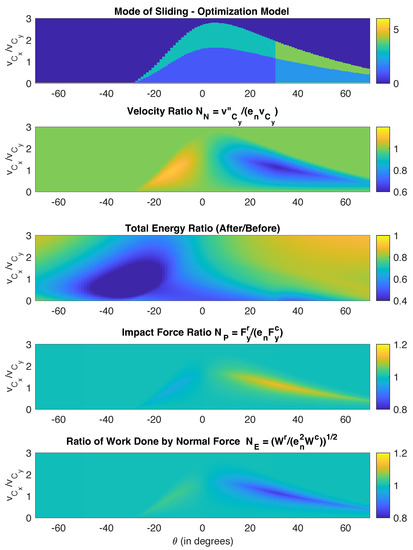
Figure 5.
Influence of orientation angle and velocity ratio on the type of impact for , , . Top figure: mode of sliding; second figure: velocity ratio ; third figure: total energy ratio (after impact/before impact); fourth figure: ratio of normal force for restitution and compression ; bottom figure: ratio of work done by normal force . Optimization model is used.
We can clearly see from Figure 5 that in both plots of the ratios and the maximum and minimum values are closer to unity than their counterparts in Figure 2 and Figure 3. That is, the plot of in Figure 5 has lower maximums and higher minimums than the plot of in Figure 2. Similarly, the plot of in Figure 5 has lower maximums and higher minimums than the plot of in Figure 3. When comparing the velocity ratio, , Figure 5 is more similar to the Poisson model than the energetic model.
We next plot in Figure 6 results when friction is increased to 0.7 while keeping the other parameters the same. We observe that the modes of motion change, velocity ratios are higher, and there is less total energy in the system after impact, all expected results. On the other hand, in contrast with earlier results for the Poisson and the energetic models, values for and do not change nearly as much, an indicator that the optimization technique leads to more consistent results for the impact forces and work done than the Poisson and energetic approaches. Similarly, the band where the impact results lose accuracy becomes wider with increased friction. The one black dot in the figures is associated with a convergence issue of the optimization procedure.
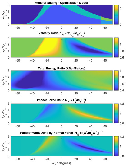
Figure 6.
Influence of orientation angle and velocity ratio on the type of impact for , , . Top figure: mode of sliding; second figure: velocity ratio ; third figure: total energy ratio (after impact/before impact); fourth figure: ratio of normal force for restitution and compression ; bottom figure: ratio of work done by normal force . Optimization model is used.
Let us next repeat the analysis for the maximum and minimum values of and for different values of the coefficients of restitution and and friction. We use the values of 0.4 and 0.8 for both these coefficients. The results for 2D impact with the same parameters as in Table 2 are shown in Table 4.
Table 4.
Minimum and maximum values for and for different values of and . The optimization approach is used to solve the impact equations.
When compared with Table 2, we observe exactly what we saw in Figure 5 and Figure 6 that the maximum and minimum values the ratios and are much closer to unity than in Table 2. The difference from Table 2 is quite striking. Values around 1.40–1.50 in Table 2 are now around 1.15, a significant drop. We conclude that the maximum and minimum values of the force ratios and energy ratios are much closer to 1 so that inconsistencies are reduced substantially.
We note that, when , the optimization results are identical to results obtained using the energetic formulation. Similarly, when , the optimization results are identical to results obtained using the Poisson formulation.
Let us next compare the simulation results by tabulating the velocities and angular velocity, as well as and , for given angles. In the first comparison, we use . In the second comparison, the incident angle is with all the other parameters the same.
In both Table 5 and Table 6, the optimization results look like the averages of the values obtained for the Poisson and energetic models. This is expected, as the optimization approach is a compromise between the Poisson and energetic approaches.
Table 5.
Post-impact values for the three models and for . Mode of motion is sticking.
Table 6.
Post-impact values for the three models and for . Mode of motion is reverse sliding.
The results also show that the velocity ratio of modeling restitution is indeed more inaccurate. Since the pre-impact value of is 1 in both Table 5 and Table 6, the vertical velocity of the contact point after impact is expected to be when the Newton model () is used. The results are and , more than a 20% difference from , larger than the differences for and .
As stated earlier, experimental results should be compared with the three analytical approaches used in this paper. Nevertheless, the optimization approach, which permits simultaneous use of both the Poisson and energetic formulations, appears to be a viable alternative that produces more consistent and realistic results.
7. Experimental Modeling of Restitution and Friction
Experimental results show that the normal force generated during impact increases with time during compression and decreases during restitution and that the time elapsed during restitution is shorter than time elapsed during compression. Figure 7 shows a generic model for such an impact force. For a triangular profile of impact lasting during compression and for restitution, the impulsive force during compression, which is the integral of the force over time, is . Similarly, the impulsive force during restitution is . As we saw earlier, the Poisson approach defines the ratio of the two impulsive forces as the coefficient of restitution. If we assume that the rise and fall profiles are linear, the coefficient of restitution becomes the ratio of the duration of restitution to duration of compression
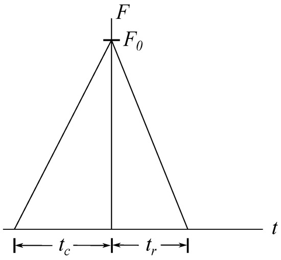
Figure 7.
Profile for an impact force.
Other impact force profiles give different expressions for the coefficient of restitution. In general, impulsive force profiles are closer to sinusoidals than straight lines [18].
Figure 8 shows an experimentally-obtained acceleration profile from a drop test of a corrugated cardboard container inside which were two ammunition boxes, encased by cushioning material made of folded paper. Reference [11] describes the process of developing the folded-paper cushioning system and the material properties of the cushion. The accelerations (in g) were measured by attaching a triaxial accelerometer to one of the ammunition boxes. The container with the ammunition boxes and cushions weighed about 45 kg and the drop height was 30 m onto a concrete ramp. The objective of the experiments was to measure the load-absorbing capability of the folded-paper cushions developed for the U.S. Army. Calculating coefficients of friction and restitution was not a primary objective. However, we can use Figure 8 for observations about and .
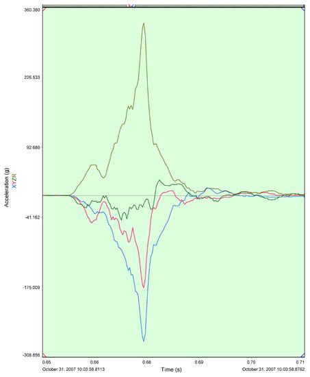
Figure 8.
Acceleration profile obtained experimentally using a triaxial accelerometer.
The acceleration profiles in the bottom half of the figure show accelerations in the different orientations of the accelerometer:
- X-direction (blue), which was close to the impact direction perpendicular to the drop surface, but not exactly. Accurately measuring orientation of the box from video of the drop was difficult. The X-direction was relatively close to the direction of the normal force, with a peak acceleration close to 300 g.
- Near horizontal Y-direction (red), along direction of sliding or impending lateral velocity (impulsive friction force direction).
- A third direction Z (green), along which there was little acceleration (compared to the other levels).
The top curve (brown) shows magnitude of the total acceleration, with the peak acceleration reaching 350 g. We note that other drop tests we conducted using similar equipment gave similar acceleration profiles. We observe the following from Figure 8:
- As expected, the restitution period is shorter than the compression period.
- A rough estimate of the coefficient of restitution is . This value is obtained by approximating the acceleration profile as consisting of straight lines. This calculation was verified by visually observing the height to which the box rose after impact.
- The impulsive friction force has almost the same form as the impulsive normal force, providing evidence for the general assumption that the coefficient of friction is constant or near-constant during impact. The coefficient of friction can be estimated by comparing magnitudes of the accelerations in the perpendicular and horizontal directions as . As mentioned above, the perpendicular and horizontal directions are approximate.
- The impact duration is about 0.03 s. Note that there is an error in the plot provided by the recording device regarding increments of time.
- The initial small rise, then drop, and then larger rise of the acceleration profile can be explained by the presence of folded-paper cushion around the ammunition case before the majority of the impact took place.
- The acceleration curves during restitution are smoother than compression.
Given the observations above, we justify describing the impulsive friction force as a friction coefficient multiplied by the impulsive normal force. On the other hand, the results do not provide justification for the assumption that the coefficient of restitution does not change with speed of impact and orientation of the impacting object.
8. Conclusions
This paper analyzes inconsistent results that can be obtained when modeling rigid body collisions via algebraic equations. While the Poisson approach leads to inconsistencies associated with the work done by these forces, the energetic model leads to inconsistencies in force ratios of compression and restitution forces. The inconsistencies are not affected by the coefficient of restitution but they increase as the coefficient of friction becomes higher. It is possible, as friction becomes larger, to obtain physically unrealizable results. It is recommended that algebraic equations for impact be used when the amount of friction in the system is low. An optimization procedure is proposed to calculate post-impact velocities and impact forces which reduces the inconsistencies associated with the magnitudes of the compression and restitution forces, as well as work done by these forces. Prior experimental results provide guidelines for modeling the coefficients of restitution and friction.
Funding
This research was funded in part by the NASA Grant 80NSSC20M0066.
Institutional Review Board Statement
Not applicable.
Informed Consent Statement
Not applicable.
Data Availability Statement
Data is contained within the article.
Conflicts of Interest
The author declares no conflict of interest.
References
- Baruh, H. Analytical Dynamics; WCB/McGraw-Hill: Boston, MA, USA, 1999. [Google Scholar]
- Pitenis, A.; Dowson, D.; Sawyer, W. Leonardo da Vinci’s Friction Experiments. Tribol. Lett. 2014, 56, 509–551. [Google Scholar] [CrossRef]
- Routh, E. The Advanced Part of a Treatise on the Dynamics of a System of Rigid Bodies; Dover Publications: Mineola, NY, USA, 1905. [Google Scholar]
- Baca, R.; Reu, P.; Aragon, D.; Brake, M.; VanGoethem, D.; Bejerano, M.; Sumali, H. A Novel Experimental Method for Measuring Coefficients of Restitution; Technical Report SAND-2016-5693 643511; USDOE National Nuclear Security Administration: Washington, DC, USA, 2016.
- Marques, F.; Wolinski, L.; Wojtyra, M.; Flores, P.; Lankarani, H. An investigation of a novel LuGre-based friction force model. Mech. Mach. Theory 2021, 166, 104493. [Google Scholar] [CrossRef]
- Keller, J. Impact with friction. J. Appl. Mech. 1986, 53, 1–5. [Google Scholar] [CrossRef]
- Stronge, W. Rigid body collisions with friction. Proc. R. Soc. Lond. Ser. A Math. Phys. Sci. 1990, 431, 169–181. [Google Scholar]
- Brogliato, B. Nonsmooth Mechanics, 3rd ed.; Springer: London, UK, 2016. [Google Scholar]
- Wang, Y.; Mason, M. Two-Dimensional Rigid-Body Collisions with Friction. J. Appl. Mech. 1992, 59, 635. [Google Scholar] [CrossRef]
- Sun, H.; Baruh, H. Analysis of Three-Dimensional Rigid-Body Impact with Friction. Dynamics 2022, 2, 1–26. [Google Scholar] [CrossRef]
- Baruh, H.; Elsayed, E. Experimental design of a folded-structure energy-absorption system. Int. J. Mater. Prod. Technol. 2018, 56, 111–127. [Google Scholar] [CrossRef]
- Djerassi, S. Three-dimensional, one-point collision with friction. Multibody Syst. Dyn. 2012, 27, 173–195. [Google Scholar] [CrossRef]
- Ling, Z.; Chong, P.; Bingyin, Z.; Wei, W. Three-dimensional modeling of granular flow impact on rigid and deformable structures. Comput. Geotech. 2016, 112, 257–271. [Google Scholar]
- Stronge, W.J. Energetically consistent calculations for oblique impact in unbalanced systems with friction. ASME J. Appl. Mech. 2015, 82, 081003. [Google Scholar] [CrossRef]
- Batlle, A. Rough balanced collision. ASME J. Appl. Mech. 1996, 23, 168–172. [Google Scholar] [CrossRef]
- Wang, L.; Zhou, W.; Ding, Z.; Li, X.; Zhang, C. Experimental determination of parameter effects on the coefficient of restitution of differently shaped maize in three-dimensions. Powder Technol. 2015, 284, 187–194. [Google Scholar] [CrossRef]
- Wang, L.; Zheng, Z.; Yu, Y.; Zhang, Z. Determination of the energetic coefficient of restitution of maize grain based on laboratory experiments and DEM simulations. Powder Technol. 2020, 362, 645–658. [Google Scholar] [CrossRef]
- Stronge, W. Impact Mechanics, 2nd ed.; Cambridge University Press: Cambridge, MA, USA, 2018. [Google Scholar]


Publisher’s Note: MDPI stays neutral with regard to jurisdictional claims in published maps and institutional affiliations. |
© 2022 by the author. Licensee MDPI, Basel, Switzerland. This article is an open access article distributed under the terms and conditions of the Creative Commons Attribution (CC BY) license (https://creativecommons.org/licenses/by/4.0/).