Article

Investigation of Jamming Phenomenon in a Direct Reduction Furnace Pellet Feed System Using the Discrete Element Method

Center for Innovation through Visualization and Simulation (CIVS) and Steel Manufacturing Simulation and Visualization Consortium (SMSVC), Purdue University Northwest, Hammond, IN 46323, USA
*
Author to whom correspondence should be addressed.
Dynamics 2023, 3(4), 711-736; https://doi.org/10.3390/dynamics3040038
Submission received: 14 September 2023 / Revised: 2 October 2023 / Accepted: 9 October 2023 / Published: 17 October 2023

Abstract

:
A continuous iron ore pellet feed system for a direct reduction ironmaking furnace is reportedly jamming in a hopper above the furnace, where a counterflowing gas seals off the furnace flue gas. The conditions that result in jamming are not well understood. The system is computationally modeled utilizing the coupled discrete element method (DEM) and computational fluid dynamics (CFD) technique. The technique is computationally expensive; therefore, the pellet sizing is modified while preserving the key metrics important in jamming. The model is used to study the impact of pellet moisture, heating, and ice formation between pellets in relation to the jamming event. The results indicate that the influence of moisture alone on the bulk shear rate is unlikely to jam the system and that insufficient heat is supplied by the counterflowing gas to raise the temperature of the pellets, which suggests freezing conditions can exist within the hopper. Particle bonding is implemented to replicate wet and icy pellets freezing and breaking up. The results indicate that the system jams in winter conditions when the hopper is charged with a minimum of 15% icy pellets, or 10% icy with 5% wet pellets. These results agree with industry reports of jamming during winter operations.

1. Introduction

Ironmaking is the most carbon-intensive step of the steelmaking process, with the steel industry being responsible for 7% of global CO2 emissions [1]. The typical ironmaking process uses carbon-based fuels, in the form of coke and natural gas, to provide both the heat and reduction gases necessary to reduce iron oxides to liquid iron in a shaft furnace called a blast furnace. Direct reduction ironmaking is becoming a popular alternative to the typical blast furnace ironmaking route due to the lower carbon impact of the process. Industrial direct reduction ironmaking is most commonly achieved by supplying hot reducing gases to iron oxides to yield a solid iron product.
Direct reduction furnace operation requires the continuous supply of iron ore, generally in the form of iron ore pellets. Continuous feed systems are generally prone to jamming of the material, which in the case of a direct reduction furnace significantly negatively impacts iron production rates. A problem sometimes encountered during winter-month operation of DRI shaft furnaces in cold-weather climates is jamming of the pellets that are charged into the continuous pellet feed system hopper. Jamming of flowing material is a common problem in industries where there is granular flow through hoppers, and many anti-clogging devices have been devised, but there is no good way to avoid jamming entirely [2]. Jamming is often studied in terms of the probability that a given flow will jam [3]. Many factors have been found to influence the likelihood of jamming, including particle roughness and shape [4,5,6,7], particle size [8], size of the outlet [9,10], container geometry [11,12,13], and particle packing [14].
Lu et al. proposed a unified theory of jamming, suggesting that the state variables that govern isothermal states of jamming are the shear rate, pressure, and free volume [15]. The isothermal state of materials refers to a non-thermal temperature, describing the “fluffiness” of the material. The research by Lu et al. agrees with studies on the subject of jamming within hoppers, which found that pressure is an important parameter [3]. The identification of the shear rate being of importance agrees with studies that found that the interparticle and particle–wall friction coefficients are important for flow states and jamming [4,5,6,7]. The importance of the free volume agrees with studies showing that the volume fraction is an important parameter in whether a granular flow will jam [6].
Jamming of flowing granular material is a complex probabilistic physical phenomenon dependent on interparticle forces. Because of the importance of particle forces, a modeling technique called the discrete element method (DEM) has been used to study how and why jamming occurs. DEM models individual particles, tracking the position, orientation, and forces acting on each particle, which allows for the modeling of granular flow and capturing of physical phenomenon that are dependent on interparticle forces, such as jamming. The use of DEM allows researchers to gather metrics that would otherwise be too difficult or impossible to obtain. For instance, Natsui et al. modeled the distribution of fines within a blast furnace, showing the distribution of fine clusters and void fractions within the furnace [16]. The pressure drop through the furnace was calculated using simulated voids and agreed with the experimental results.
Research by Xiao et al. showed that how particles jam through a bottleneck is via the formation of an arch around the outlet [2], and that arch formation could form through two different mechanisms. Research by Park et al. showed that increasing pressure near the outlet of a hopper increases the probability of arch formation [3]. Both Xiao’s and Park’s studies used DEM to carry out their research. The work of Ketterhagen et al. shows that flow patterns within hoppers can be successfully predicted using DEM [17]. The results were validated against the experimental work of Jenike, who described the flow patterns that exist within hoppers given certain flow conditions and hopper geometries [18].
Discrete element modeling has been used to replicate the bulk flow behavior of iron ore pellets by researchers such as Li et al. and Barrios et al. The discrete element method was used by Li et al. to replicate the experimental piling behavior of iron ore pellets [19], using spherical particles and calibrated friction coefficients to match bulk flow behavior against the experimental results. Barrios et al. used DEM to show that pellet contact parameters could be used directly to simulate the bulk flow behavior of pellets if the geometry of the pellets was accounted for [20]. They also showed that friction coefficients must be calibrated to replicate the bulk flow if perfect spheres are used to reduce the computational cost of the simulation.
DEM can also be coupled with CFD to model the exchange of mass momentum and energy between fluid and solid phases. Work by Che et al. showed that two-way coupled DEM-CFD simulations are able to replicate the dynamics of particles in a sprouted bed [21], and their work was validated against experimental data that tracked the motion of particles. Using the two-way coupled technique, Wang et al. were able to determine that the dominate mode of heat transfer in a fluidized bed is convection, with conduction being negligible [22]. Their work was validated against the experimental literature results [22,23]. The two-way coupled technique was also used by Kinaci et al. to model a direct reduction in iron ore in a fluidized bed accounting for mass, momentum, and heat transfer between the solid and fluid phases. Their simulation results agreed with experimental data on the time to and degree of reduction, and the predicted rate limiting step agreed with other data from the literature [24]. The discrete element method can be used to simulate bonding between particles and allows for the control of the bond strength by specifying the tensile and shear strength of the bond. This method has been used to replicate the mechanics of ice break up [25]. In a study by Di et al., this technique was used to predict the forces necessary to break up arctic sea ice, and the results were validated against ISO sea ice force standards [25]. Jou et al. investigated ice breaking by icebreaker ships using the same method and concluded that the bonded DEM method can accurately capture ice fracture physics [26].
Despite the advantages of using DEM, it is inherently a computationally expensive model, which imposes limits on large simulations with many particles [27]. Physical properties of the particles, such as shape or size distribution, can be altered to reduce computational expense, but it is important that the bulk flow characteristics of the material are matched against the experimental results by calibrating the contact parameters between particles [20,27]. The success of DEM in simulating bulk granular flow behavior within hoppers, and of iron ore pellets, along with its usefulness in studying the jamming of granular flow, make it a suitable method for replicating the flow of pellets in a direct reduction ironmaking furnace feed system and capturing jamming of the flow. Further, the success of coupled DEM-CFD in replicating momentum and heat transfer in packed and fluidized beds between solid and fluid phases, combined with the successful modeling of ice break up and bonding, makes it a suitable technique for investigating jamming in an iron ore feed system exposed to wet and freezing conditions.
This research addresses a crucial yet understudied issue in the operation of DRI furnace feed systems, which is the jamming of iron ore pellets, particularly during operation in freezing winter conditions. This is accomplished by exploring the jamming of granular flow due to freezing conditions by combining simulation techniques that have proven valuable in studying the jamming of granular flow, heat transfer in dense granular flows, and ice break up mechanics. By investigating the cause of jamming in this specific context, this study potentially opens up new avenues for preventing and mitigating jamming, ensuring continual operation of the DRI furnace and supporting the steel industry’s decarbonization efforts.

2. Methodology

2.1. Governing Equations

2.1.1. Discrete Phase Equations

The Hertz–Mindlin contact model is used to resolve the normal and tangential forces acting on each particle. The model treats the normal and tangential components of the force for each particle interaction as a pair of spring-dashpot oscillators, where the spring accounts for the elastic, and the dashpot accounts for the energy dissipation component of the force.
Conservation of momentum is applied to each particle as:
m i d v i d t = j F i j + F g
where F i j = F n + F t , m i and v i are the mass and velocity of particle i, respectively. The force of gravity and the force on particle i exerted by j are denoted as F g and F i j , respectively. The normal and tangential force components of F i j are denoted as F n and F t , respectively.
Similarly, the conservation of angular momentum is applied to each particle as:
d d t I i ω i = j τ i j
where τ i j = r i j F i j , I i , and ω i are the mass moment of inertia, angular momentum of particle i, respectively, and τ i j is the torque exerted on particle i from j. The term r i j represents the radial distance from the center of particle i to contact with particle j.
Conservation of energy is applied to each particle with the equation given as:
m p c p d T d t = Q t + Q r a d + Q s
where m p and c p are the mass and specific heat of the particle, respectively. The term d T d t is the time rate of change in the particle temperature. The terms Q t , Q r a d , and Q s are the convective, radiative, and other heat sources heat transfer terms.
With convective heat transfer between the fluid and solid phases defined as:
Q t = h A ( T T p )
where h is the convective heat transfer coefficient, A is the surface area of the particle, T is the local fluid temperature, and T p is the particle temperature.
The chosen Nusselt number relation for heat transfer between the particles and the fluid phase has been shown to produce validated heat transfer simulation results for both fluidized and packed beds [28]. The Nusselt number relation selected for determination of the heat transfer coefficient is:
N u p = 2.0 + 1.2 R e p 1 / 2 P r 1 / 3
h = N u p k D p
where N u p , R e p , and P r 1 / 3 are the particle Nusselt number, particle Reynold’s number, and fluid Prantel number, respectively. The terms h , k , and D p represent the heat transfer coefficient, the fluid thermal conductivity, and the particle diameter.
Boundary layers around the particles are not resolved in coupled DEM/CFD simulations; instead, local continuous phase flow field properties are applied to the particle, and the particle takes up a portion of the volume of a cell that the cell treats as a void. Rather than modeling drag on each particle via boundary layer effects, the drag exerted on the particles is determined by calculating the drag coefficient using the local flow field velocity. The flow field velocity is affected by the occupation of a percentage of each shared cell by particles, represented as a void to the fluid. The Di-Felice drag coefficient is formulated considering the boundary layer effects of nearby particles through the local void fraction.
The drag force is given as:
F d = 1 2 C d ρ A p v s v s
where F d is the drag force, C d is the drag coefficient, ρ is the fluid density, A p is the particle surface area, and v s is the fluid velocity.
With the Di-Felice drag coefficient defined as:
C d = 0.63 + 4.8 ϵ R e p 2 ϵ 2 ζ
where ζ = 3.7 0.65 e x p 0.5 ( 1.5 l o g ϵ R e ) 2 , ϵ is the void fraction, and R e p is the particle Renold’s number.
Bonding between particles in contact is modeled using the principles of basic beam failure theory, and as a method has proven useful in both modeling of rock behavior [29] and ice break up mechanics [25,26]. The bond is treated as a beam between the particles at the point of contact, and the bond is given a shear and tensile failure strength. The maximal tensile stress that the bond experiences is defined as [29]:
δ m = F n A + M s R I
The maximal shear stress that the bond experiences is defined as [29]:
σ m = F s A + M n R J
where F n and M n are the normal components of the force and torque, respectively. The terms F s and M s are the shear components of the force, respectively. The terms I , J , A , and R are the second moment of area, second polar moment of area, cross-sectional area, and radius, respectively. Failure of the bond occurs when the maximal shear ( σ m a x ) or tensile strength ( δ m a x ) is exceeded, namely failure when δ m > δ m a x or σ m > σ m a x .

2.1.2. Continuous Phase Equations

Mass, momentum, and energy are conserved for the fluid phase. Energy and momentum are exchanged between the phases, while mass is not exchanged.
To model the conservation of mass, the continuity equation is given as:
ρ t + . ρ u i = 0
where time, fluid density, and fluid velocity are denoted as t , ρ , and u i , respectively.
Conservation of momentum in the fluid phase is given as:
x ρ u i + . ρ u i u i = p + . τ + ρ g i + F
where τ is the stress tensor, F is the body force exerted on the fluid, and g i is gravitational acceleration in the i direction.
Conservation of energy for the fluid phase is given as:
ρ c D T D t = k 2 T + Φ
with c , T , and k as the fluid specific heat, temperature, and thermal conductivity, respectively. The energy dissipation rate is denoted Φ and defined as:
Φ = μ u i u j + u j u i u i x j
The k-epsilon turbulence model is commonly used in CFD applications to model turbulent fluid motion and has been shown to be suitable for use in coupled DEM/CFD dense granular flow simulations [30]. The two variables k and ε represent the fluid kinetic energy and the dissipation of that energy, respectively.
The k equation is given as:
t ρ k + . ρ k v ¯ = . μ + μ t σ k k + P k ρ ε ε 0 + S k
The ε equation is given as:
t ρ ε + . ρ ε v ¯ = . μ + μ t σ k ε + 1 T e C ε 1 P ε C ε 2 f 2 ρ ε T e + ε 0 T 0 + S ε
where P k and P ε are the kinetic and dissipation production rates, respectively, and C ε 1 and C ε 2 are the model coefficients. The terms S k and S ε are source terms for the kinetic energy and dissipation rate, respectively. The terms T e , T 0 , and f 2 are the eddy timescale, ambient turbulence timescale, and the damping function.

2.2. Set Up of Simulations in STAR-CCM+

The computational demands of this study are high due to the large number of tracked particles required to simulate the DRI feed system process. For this reason, the software STAR-CCM+ was chosen as it is capable of good performance and scalability.
The physical models selected during setup of the simulations that govern the interactions of the fluid and solid phases are the Lagrangian multiphase model with DEM option enabled, two-way coupling, and the drag force model. The models selected to govern the modeling of particle interactions and forces are the Hertz–Mindlin model, the DEM boundary force model, which tracks forces exerted on the walls, and the parallel bonds model for when the bonding of particles is considered. When heating of the pellets is simulated, the energy equation is enabled, with the heat transfer coefficient manually defined to govern heat exchange between the fluid and solid phase.
The case setup starts by the generation of the grid. For DEM/CFD coupled simulations, a constraint on the grid sizing is that the cell size must be larger than the pellet diameter. It is common in DEM/CFD coupled simulations to use a cell to diameter size ratio of 3 [31], with multiple studies showing a minimum ratio of 1.6 [31,32], and some to a maximum of 4 [33]. The cell size to diameter ratio used in this study is approximately 3, relative to the average particle size used in simulations, and approximately 2, relative to the largest particle size.
Once the computational domain is generated in the program, the case-specific physics model options are selected, and the simulations are conducted in these stages:
  • Define case-specific pellet material properties;
  • Define boundary conditions;
  • Fill domain with ore pellets;
  • Start simulation allowing gas and pellets to flow.

2.3. Pellet Bulk Flow Validation

The discrete element method is used to model the bulk flow of iron ore pellets, with the pellets modeled as perfect spheres. To account for the effect of individual pellet shapes on the pellet bulk flow behavior in the DEM simulation, the friction is calibrated so that the results of a drop test for iron ore pellets of different sizes, originally performed by Li et al. [19], are replicated. The test is performed by dropping pellets of different diameter sizes 5 times each and recording the average left and right angle of repose, which is the angle between the steepest slope of a stacked pile of granular material and the horizontal plane it rests on, shown in Figure 1. During testing, the angle of repose is measured as the slope at which the simulated iron ore pellets come to rest after being dropped in a pile, shown as the red angle in Figure 1. Calibration of friction coefficients by replication of the angle of repose is useful because the angle of repose is dependent on the bulk flow properties of the pellets. Specifically, it is influenced by the kinetic energy dissipation of the pellets [19] and the pellets ability to form stables structures under the force of gravity. Both of these bulk flow properties are influenced by the individual particle geometry [20], which is not counted for when using perfectly spherical particles, and is therefore a valid metric to calibrate against [20].
The friction values between the pellets and the walls of the drop test are assigned as the steel–pellet friction parameters that Barrio’s et al. found to replicate pellet behavior against steel walls [20] using DEM and spherical particles. The pellet–pellet contact static and rolling friction coefficients that are found to replicate the experimental angle of repose results are 0.50 and 0.20, respectively. The static and rolling coefficients between pellet–pellet contacts and pellet–steel contacts that reproduced the experimental angle of repose with a changing pellet size are shown in Table 1.
The values for the left and right angle of repose verses the size of the particle for both the simulation and the original experiment are shown in Table 2. Three pellet sizes, 5.5, 7.0, and 9.0 mm, are simulated and compared to three pellet sizes, 5.0, 7.0, and 9.0 mm, from the experimental data. The minimum pellet diameter for the simulations was 5.5 mm, whereas the minimum diameter in the experimental data was 5.0 mm. This was to reduce the computational cost of the simulations while still validating the trend for the angle of repose with different pellet sizes, as smaller diameters lead to more pellets and higher computational cost. The resulting linear trend for the angle of repose verses the size of the pellet matched that of the experimental results, suggesting that the calibrated friction parameters accurately capture the effect of pellet shape on the bulk flow, as shown in Figure 2 and Figure 3. In both the experimental and simulation data, it can be seen that as the pellets increase in diameter, the angle of repose decreases. This is because the kinetic energy of the smaller pellets dissipates faster than that of larger pellets, which is likely due to increased interparticle contacts, resulting in the increased packing stability of the pellets [19]. Agreement between the experimental and simulation results suggests that the bulk flow behavior of the spherical DEM pellets is calibrated to that of actual iron ore pellets.

2.4. Feed System Model

The feed system hopper and flow aid insert are modeled with the approximate dimensions and boundary conditions shown in Figure 4. The domain was created using symmetry conditions dividing the hopper into a third along its longitudinal axis. The top outlet of the hopper is a pressure outlet at atmospheric pressure, and the bottom serves both as a gas velocity inlet set at 1.91 m/s and an outlet for the ore that limits the maximum mass flow rate to the operational feed rate into the furnace. The domain is meshed using a cell size of 0.07 m and is shown in Figure 5.
The normal operation of the feed system is modeled as the baseline case. To reduce the computational expense of the model, the height of the upper portion of the hopper is reduced, and a layer of larger particles that are 10× denser than the ore pellets are modeled atop the descending pellet bed to replicate the weight of the full fill height, as shown in Figure 6. The pellet void fraction and velocities are tracked near the upper and lower portions of the flow aid (highlighted in Figure 6) where jamming is reportedly happening.

2.5. Pellet/Gas Properties and Contact Parameters

The pellet material and thermal properties used in the study are shown in Table 3, and the gas density and dynamic viscosity used for the simulations are shown in Table 4.
The contact parameters used between pellets and between the pellets and steel for the cases are shown in Table 5. The pellet–pellet static and rolling coefficients are determined by matching the drop test simulation angle of repose values with the experimental results by Li et al. [19] and are used in both the baseline case and the charged icy/wet pellets cases. The friction coefficients are increased for the high moisture case to enhance the assumed effect of increased resistance to shear in the bulk flow due to moisture. The high friction coefficients are not applied to the icy/wet charged pellets cases and instead use the baseline coefficients to isolate the effect of bonding due to freezing on the pellet bulk flow.
The number of particles needed to simulate the pellets within the full hopper, without including the modeling of fines, is on the order of 100 million. Given that DEM models the position, orientation, and forces on every particle, modeling this number of particles greatly exceeded the computational resource capabilities available for this study. To model the hopper using DEM, and capture jamming of the system without exceeding the computational limits, the particle number is to be reduced, and the bulk flow characteristics that are important with respect to jam formation are to be maintained.

3. Results

3.1. Computational Cost Management

To reduce the computational cost of simulating a high number of pellets in the feed system while maintaining the key parameters involved in jamming, a parametric study was conducted on a hopper with reduced dimensions (Figure 7). The smaller hopper is conical and axisymmetric. In this simulation, the hopper is first charged with pellets that are the size of the operational normal pellet diameter distribution, with mean pellet size being at approximately 10 mm. The pellets are then discharged with no restriction of the pellet flow rate. The void fraction and pellet velocity are tracked, as they are the primary parameters involved in jamming [2,15], along with the amount of time elapsed per iteration of the simulation. The pellet size and distribution are then parameterized, and the use of symmetry conditions is implemented. The change in the relevant bulk flow metrics and simulation time are measured and compared to the first case which uses the full reduced hopper geometry and actual pellet size distribution, which is termed the reduced baseline case. This is to determine what conditions optimally conserved the metrics while sufficiently lowering the computational expense of the model.
The top of the hopper is a pressure outlet at 1 atm, and the bottom of the hopper is a gas velocity inlet injecting air at 1 m/s and an outlet for the pellets. The metrics are tracked in the narrowing cone-shaped region of the hopper. The hopper boundary conditions are shown in Figure 8A.
Multiple cases were tested parameterizing the pellet diameter size between 1 and 2× the original size and varying the shape of the pellet diameter size distribution between a uniform and normal distribution. The impact of using one third the domain, shown in Figure 8B, by use of symmetry conditions is explored in combination with the pellet size changes.
With the final selected simulation assumptions, the time elapsed per iteration for the simulation was reduced by 97.9%. This is accomplished by using a normal pellet size distribution with the pellet diameter scaled 2× the original normal size distribution, and by implementing symmetry conditions to divide the domain into thirds. The relevant pellet bulk flow parameters are well maintained, with the void fraction increasing from the original test case by 3.17% and the mean pellet velocity decreasing by 12.85%. The change in pellet velocity has less impact on the furnace feed system simulations because the descent rate of the pellets is governed by the pellet feed rate into the furnace, as opposed to the unimpeded discharging in the cost reduction tests. Table 6 shows the resulting conditions for the computationally efficient case, determined from the parametric testing, that can be implemented to reduce computational expense without compromising bulk flow characteristics, and compares them to the baseline conditions. Table 7 shows the resulting change in granular bulk flow characteristics between the two cases, along with the computational cost in terms of the time elapsed per iteration.

3.2. Baseline Operation

3.2.1. Forces on Walls

The baseline operation results indicated that the location of higher forces on the walls and flow aid insert within the hopper appear where industrial hopper jamming has been observed at a height above the top half of the flow aid, as shown in Figure 9A,B. The forces are higher on the upper portion of the flow aid and are lower below the widest part of the flow aid where the flow aid narrows. The higher forces on the top of the flow aid and on the walls in this region are consistent with an increased probability of jamming in this region.

3.2.2. Void Fraction and Pellet Velocity

A contour of the void fraction is shown in Figure 10 and shows that the void fraction increases as the pellets descend through the hopper. Likewise, the velocity of the pellets is shown in Figure 11 showing an increase as they descend through the hopper. The increased velocity of the pellets is expected as the cross-sectional area of the hopper is decreasing while the mass flow rate of the pellets remains constant. The corresponding increase in the void fraction as the pellets descend is also expected as the increasing kinetic energy of the pellets, and the rolling of pellets over each other in a reducing cross-sectional area creates more space between the pellets. At the same time, the flow aid insert interrupts the flow, supporting the weight of the pellets above it and increasing the void beneath it. The average velocity of the pellets and the average void fraction are both lower in the upper flow aid region when compared to the lower flow aid region (regions highlighted in Figure 6), indicating that the upper flow aid region is more prone to jamming than below. This is also consistent with where the forces suggest jamming is most likely to occur. Table 8 shows the values of the average void and average velocity of the pellets in both regions.

3.3. Operation during High Moisture Conditions

3.3.1. Moisture Level and Impact on Bulk Flow Behavior

Pellets are exposed to year-round environmental conditions before charging, and depending on the facility’s local climate, pellets can be exposed to freezing and wet weather conditions for extended periods of time. The effect of high moisture content in the charged pellets is explored using the same methodology as the baseline case, but with an assumed higher friction between the pellets.
Iron ore pellets have been shown to hold a maximum moisture content of 5.5% the mass of the pellets when soaked [34]. However, the impact of moisture levels on pellet contact parameters and on the bulk flow behavior of the pellets is not well documented. In contrast, the bulk flow behavior of iron ore fines in relation to specific moisture levels has been studied, and it has been found that the flowability of the fines decreases significantly at moisture levels between 3 and 12% the mass of the fines [36]. The decreased flowability of the fines is due to the interparticle cohesive forces that are caused by the surface tension of the liquid bridges between the particles [36]. The strength of the liquid bridges being significant relative to the weight and size of the particle reduce the bulk flow resistance to shear [37]. The fines resistance to shear increases dramatically for increasing moisture levels between 0 and 3% and stays relatively constant between 3 and 12% moisture levels. Data for the impact of moisture levels higher than this in relation to bulk flow behavior are sparse; however, it is known that when moisture levels become high enough, granular materials become suspended in the fluid, and the cohesive effect of liquid bridges is lost. Moisture levels within the feed system that are high enough to suspend the particles are highly unlikely. Given that the pellets can hold a maximum of 5.5% their mass as moisture, and the pellets make up the majority of the mass in the system, it is reasonable to assume that a high moisture level in the system for pellets and fines is 5.5% the mass of them both. So, for this study, when high moisture in the feed is referenced, it is referencing a 5.5% mass moisture level of the pellets and fines.
Given that the combined bulk flow effects of moisture on both fines and pellets together are not well documented, this study assumes that the net bulk flow effect of moisture (at a level of 5.5% the mass of the charge) with fines on the charged pellets is an increased resistance to shear stress. To investigate the potential impacts of this increased resistance, the rolling and sliding friction coefficient assumptions are significantly increased for these test scenarios, both to a value of 0.9. This proof-of-concept is intended to explore whether a significant increase in friction due to moisture might explain jamming phenomena, regardless of the exact correlation between friction coefficients and moisture content, which is as yet unknown.

3.3.2. Forces on Walls

Friction levels in granular flow are positively correlated with the probability of jamming; however, no jam formation is captured during simulation with high friction coefficients. The high moisture scenario, which assumes 5.5% moisture level, showed a similar pattern of forces exerted on the walls and flow aid insert as found in the baseline operation, shown in Figure 12 and Figure 13. The forces on the flow aid are higher above the maximum width of the flow aid, as pointed to in Figure 12. The location of the highest average forces on the hopper walls is lowered for the high moisture scenario and decreased more rapidly as the pellets descended near the flow aid, as shown in Figure 14. This is because the increased friction forces change how the forces are distributed within the bed of pellets, impacting the location and distribution of the forces exerted on the walls. However, in both cases, the forces are higher above the flow aid and rapidly decrease below.

3.3.3. Void Fraction and Pellet Velocity

The void fraction within the hopper increases as the pellets descend for both cases; however, the void fraction increases significantly more when accounting for the assumed impact of moisture on friction compared to baseline operation, as shown in Figure 15. Like the baseline case, the increase in the void fraction as the pellets descend is because the increased kinetic energy of the pellets creates more space between the pellets, along with the pellets rolling over each other in a decreasing cross-sectional area, increasing the void space between pellets. Also, the flow aid insert interrupts the flow and supports the weight of the pellets above it, increasing the void beneath it. However, the more dramatic increase in void fraction in the high moisture scenario is because the stronger friction forces between the pellets causes them not to slip as much into the void spaces. The similar behavior of the pellets, but with a more dramatic impact on void fraction, can be seen in Figure 16; for both cases, the void fraction increases as the pellets descend until the pellets reach the widest point of the flow aid insert, where the void fraction begins to decrease and then increases rapidly again below this point.
It can be seen in Figure 17 that the pellet velocity is lower throughout the hopper when compared to the baseline case, with the difference being most apparent above the flow aid and near the exit. A decrease in pellet velocity is expected as the increased friction between pellets creates a high resistance to shear on the bulk flow level of the pellets. Above the flow aid, the pellet velocity is higher during baseline operation and then lowers near the widest part of the flow aid, where the velocity is the same for both scenarios, as shown in Figure 18. Beyond this point, near the lower flow aid and below, the velocity of the pellets increases much more in the baseline than what is seen when moisture is present.
Figure 18 shows that for both cases, the velocity of the pellets increases in a non-linear fashion as the pellets descend below the flow aid; however, for the high moisture scenario, the magnitude of the increase is less. Namely, the assumed increase in friction due to the moisture content in the pellets reduces their average velocity near the outlet by 41% with respect to the baseline case. In Figure 18, for the baseline case, it can be seen that the pellets are increasing in velocity as they descend through the upper portion of the hopper until the pellets approach the upper portion of the flow aid. The baseline pellet velocity then decreases as the flow aid obstructs the flow until the pellets pass the widest part of the flow aid; however, this is not seen in the high moisture scenario. For the high moisture case, the decrease in velocity due to the upper flow aid obstructing the flow is not seen; rather, a small increase in the velocity is seen until it reaches the max flow aid width, where the rate of increasing velocity lowers and then continues to increase dramatically.
The average velocity of the pellets in the high moisture case is 46.2% lower than that of the baseline for the upper flow aid region and 49.5% lower than that of the baseline in the lower flow aid region. The average void fraction increases by 22.2% in the upper flow aid region and by 23.1% in the lower flow aid region when compared to the baseline, as shown in Table 9.
The lower pellet velocity indicates that operating with moist pellets may increase the probability of jamming if moisture increases pellet–pellet friction forces; however, the lower forces on the flow aid and higher void fraction indicate a lower probability of jamming. The void fraction is increased in the high moisture case because with higher friction, the pellets do not slip as easily to fill the void space and pack as densely, and the lower velocity is due to the increased resistance to shear stress in the bulk flow. The change in force distribution on the walls and flow aid of the hopper is likely due to the changed bulk flow behavior influencing the shape of the granular force chains throughout the moving bed.

4. Discussion

4.1. Pellet Temperature Profile

The previously discussed modeling indicates that even if moisture content results in increased friction between pellets, flow jamming is not observed with the associated pellets (including all specified assumptions). Given that jamming has been reported by operators in cold climates during winter months, and that moisture in the feed may be present year round, moisture is unlikely to be the only factor involved in jamming. Therefore, the effect of temperature in concert with pellet moisture generating icy/frozen pellet bonds was also considered in this study.
The heating of iron ore pellets within the hopper due to the counter-current seal leg gas flow is explored using the simplified test hopper (Figure 8B). The gas to ore mass flow ratio is the same as the normal operation of the feed system, with flow rates adjusted proportionally to the mass difference between the small hopper case and the baseline case. The operational temperature of the counter current gas is 100 °C and is used for the heating gas, and the pellets are tested at a temperature just below the freezing point of water at −1 °C. The pellets in this test are assumed to have no moisture content and use the thermal properties of iron ore pellets.
The results showed that the heat transferred from the gas to the pellets quickly leaves the domain as the pellets discharge from the hopper. The heating gas does not supply enough sensible heat to significantly change the temperature of the pellets within the hopper, as shown in Figure 19, and quickly approaches the bulk temperature of the pellets (−1 °C) as the pellets leave the domain. This suggest that freezing conditions may exist in the feed system when charged with pellets at low temperatures, which would be a common scenario in many climates during winter operation, as the pellets are exposed to weather conditions outside.
The pellets tested use the thermal properties of iron ore pellets and are assumed to contain 0% moisture. If the moisture content is higher, more energy would be required to heat the pellets as water has a much higher specific heat value [34]. Further energy would be required to overcome the latent heat of fusion for melting ice. Considering these findings, it appears plausible that sub-freezing conditions in the solid phase could persist to a significant depth within the feed system and that pellets charged in a wet and icy state may form ice bonds which could contribute to flow jamming.

4.2. Jamming Due to Freezing Conditions

4.2.1. Modeling Freezing of Wet and Icy Pellets

If it is assumed that freezing conditions are present in the hopper, and that a certain content of moisture suspended with the pellets (either pre-frozen or freezing) will be required for icy bonds to be observed, an exploration can be conducted of the minimum amount of icy and wet pellets required to influence the solid flow in the feed system. A wet pellet is defined as a pellet that is soaked (additional mass water of 5.5%) above freezing temperature, and an icy pellet is defined as a soaked pellet that is below freezing temperature. Wet, icy, and dry pellets are charged into the hopper and are defined in the simulation by their ability to form bonds. These pellets are representative of material charged from different regions of the ore stock yard. Icy pellets are wet and pre-frozen from the stock yard, with any moisture present allowing ice to bond to other icy pellets. Icy pellets (sub-freezing) are also assumed to bond with wet pellets as the wet pellets contain enough moisture to form a bond when in contact with a cold pellet. Wet pellets are not assumed to directly bond with other wet pellets, and dry pellets are assumed to be both dry and warm enough so as not to bond with any other pellets (a visual aid is provided in Figure 20 for clarity). The bond shear and tensile strength between the pellets are set equal to that of ice, as shown in Table 10. It is worth noting here that this assumption of bond strength may have a significant impact on the total moisture content required to interrupt regular flow, as weaker or stronger icy bonds (both ice strength and ice–pellet strength, from a combination of fines and ice) may result from different conditions. The friction between the pellets in this case is set to be the same as the baseline. This is so the bulk flow impact of bonding due to freezing is isolated, without applying the assumed large increase in resistance to shear. Additionally, for this analysis, no thermal model is applied as the impact of heating was previously found to be insignificant.
To model and vary the percentage of icy and wet pellets charged into the hopper, the baseline case methodology was repeated, but with five additional discrete element phases added to the hopper above the flow aid insert. Figure 21 shows the feed system filled with the five additional discrete phases in blue, where the percent dry, icy, and wet pellets will be defined. In Figure 21 the grey pellets below the blue represent dry non-frozen pellets, and the red pellets above represent the heavy pellets that replicate the weight of the pellets in the full hopper fill height, as is the case in the baseline and high moisture cases (see Section 2.4). The five additional discrete phases allow for control of what percent of the pellets are frozen, wet, or dry, and are distributed evenly through this region. The amount of icy and wet pellets charged were parameterized to determine what the minimal amount of each in the charge is required to produce a jam. It is assumed that the wet and icy pellets hold 5.5% of their dry mass in moisture content, which was found by Petrich et al. to be the maximum amount [34], and the total moisture content in the charge is calculated.

4.2.2. Minimal Amount of Icy and Wet Pellets to Jam the Flow

Ice bonds forming between pellets in the flow resulted in jamming of the feed system at varying amounts of charged dry, icy, and wet pellets, as shown in Figure 22. The system is jammed where the pellet velocity is zero. Higher levels of icy and wet pellets jam the system above the flow aid, forming a large blockage, as seen in Figure 22B. Lower levels of icy and wet pellets jam the flow by also forming a blockage above the flow aid, but some of the icy and wet pellets that are not a part of the blockage descend slowly through the domain out of the hopper as they form bonds, which is seen in Figure 22C and Figure 23.
Figure 23 shows the average pellet velocity through the height of the hopper for the baseline (blue curve) and two scenarios, one with 33% icy, wet, and dry pellets (orange curve), and one with 10% icy, 5% wet, and 85% dry pellets (grey curve). Specifically, considering that 10% of the pellets are frozen and 5% are wet (grey curve), the pellet velocity reduces with respect to the baseline in the entire domain. The velocity is reduced to −85% of the baseline velocity near the exit of the domain. By further increasing the number of frozen pellets to 33% and wet pellets to 33% (orange curve), the results in Figure 22B show that the pellets do not behave as a continuous granular flow, but instead they show two regions, one region where the charged wet and icy pellets are jammed and a lower region where the dry pellets continue to flow out the domain at the operational feed rate. Figure 23 shows this jump in the pellet velocity as a discontinuity in the plot around 0.4 of normalized height.
The minimal percentage of icy pellets (pellets containing 5.5% of their dry mass in frozen water as ice) charged with dry pellets to jam the flow was found to be roughly 15% of the charged pellets. In scenarios when 10% of the charged pellets are icy, pellet flow can still be observed, but upon an additional 5% charge of wet pellets (pellets containing 5.5% of their dry mass in liquid water, able to freeze with icy pellets but not each other), the flow jams. For both cases, the total moisture in the charge is calculated to be 0.818% of the mass of the total charge (85% of the charge is dry, with 15% of the charge containing 5.5% moisture, either wet or frozen), as shown in Table 11.
The minimal mass moisture percentage of the charge that produces a jam is under the assumption that the wet and icy pellets are soaked and holding 5.5% of their mass in moisture, and that the dry pellets contain 0% moisture. This may be a reasonable assumption for estimated calculations, but it needs to be confirmed experimentally. This assumption also does not consider additional ice frozen on the pellet or charged with the pellets. Operators may be able to monitor pellet feed moisture to provide prior warning should the feed meet or exceed the 5.5% metric for a significant length of time during winter months in cold regions. Based on these results, if a minimum of 15% of the material within the hopper meets or exceeds this 5.5% moisture level during freezing weather conditions, and two thirds of the soaked material is already frozen, precautions to avoid jamming may need to be taken. This translates to 0.818% moisture content in the bulk flow when divided amongst the wet and dry material, which may appear manageable, but local conditions (based on spatial variations in moisture content in the ore field from which raw material is charged) may far exceed this level, resulting in jamming. These conditions may easily occur in wet winter months in geographical regions experiencing snowfall, particularly when outdoor stock yards are subjected to intermittent periods of near and sub-freezing temperatures.
It should be noted that the simulations detailed herein do not account for the dynamic and geometric effect of fines present in the flow due to the immense computational cost of simulating fines in such a flow. The bulk flow effects of fines present in the flow of iron ore pellets, in dry, moist, and icy/moist conditions, should be explored experimentally, along with their effect on jamming and arch formation. Another key assumption in these simulations is that icy–wet or icy–icy contact always results in icy bond formation between the pellets. It is likely that only a fraction of the contacts with the potential to form icy bonds actually do form a bond, which would imply that real-world conditions would require higher levels of wet and icy pellets charged to result in flow jamming. However, as extremely steep repose angles have been observed in raw material stock yards in winter months, it is likely that a not insignificant amount of ice could be charged into the feed system under cold and wet weather conditions. It is also assumed that the icy bonds that form between pellets have the shear and tensile strength of ice, but given that the ice bonds would likely contain fines and the strength of the ice pellet interface is unknown, this may be an inaccurate estimation of bond strength. Experimental work may be required to determine the probability of icy bonds being made in a descending bed of icy and wet pellets in freezing conditions and to make a determination of the strength of the bonds.

5. Conclusions

Based on the simulations conducted and prior analysis, the conclusions drawn from this study are as follows:
  • To reduce computational expense to a reasonable level using DEM, it was determined that the important bulk flow parameters for the formation of jams in hoppers, void fraction, and particle velocity could be maintained near original values (3.17% higher and 12.85% lower, respectively) by doubling pellet diameter and implementing symmetry conditions.
  • Above and near the top of the flow aid, the forces on the walls are higher, the void fraction is lower, and the pellet velocity is lower, indicating that this region is more prone to jamming and consistent with where feed system jamming has been reported in industrial operations.
  • Moisture and its impact on bulk flow is likely not the sole cause of jamming within the system based on aforementioned assumptions.
  • During frigid winter conditions, not enough sensible heat is supplied by the counter flowing seal leg gas to significantly impact the temperature of the iron ore pellets; therefore, it is likely that freezing conditions can exist within the feed system.
  • A minimum of 15% icy pellets (at an assumed moisture content of 5.5% of dry weight) charged reduces the velocity of the pellets and produces a jam in the system, or 10% icy with 5% wet pellets. Similarly, levels of icy and wet pellets each in the range of 33% of the feed cause the system to jam by the formation of a large blockage.
Finally, it should be noted that experimental work on moist pellet contact parameters, bulk flow effects of fines and pellets as they relate to jamming in wet and dry conditions, and icy bond formation and strength between pellets are likely necessary to confirm the assumptions made in this study. Further work could utilize such investigations to assess the likelihood of jamming in real-world operation conditions specific to a given facility or system.

Author Contributions

Conceptualization, T.O. and J.G.R.; methodology, T.O. and J.G.R.; software, J.G.R.; validation, J.G.R.; formal analysis, J.G.R., T.O. and O.J.U.; investigation, J.G.R.; resources, T.O. and C.Q.Z.; data curation, J.G.R.; writing—original draft preparation, J.G.R.; writing—review and editing, O.J.U., T.O. and J.G.R.; visualization, J.G.R.; supervision, T.O.; project administration, T.O. and C.Q.Z.; funding acquisition, T.O. and C.Q.Z. All authors have read and agreed to the published version of the manuscript.
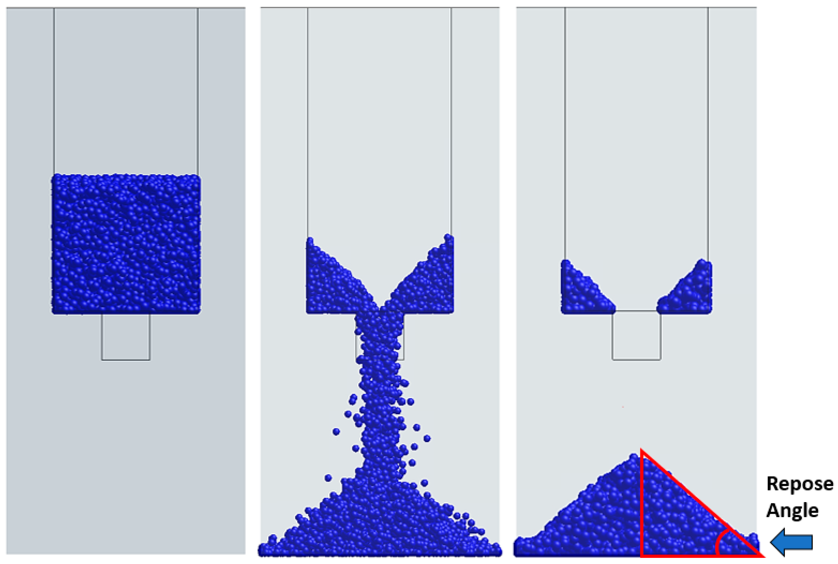
Funding

This research received no external funding.

Data Availability Statement

Simulation data for generic geometries and operating conditions may be made available upon request of the authors. Simulation data pertaining to industrial operations is protected by confidentiality, and may only be shared with the permission of industrial partners within the Steel Manufacturing Simulation and Visualization Consortium.

Acknowledgments

The authors would like to thank the members of the Steel Manufacturing Simulation and Visualization Consortium (SMSVC) for their technical support and guidance during development of the models utilized in this study. Support from individual industry collaborators and staff and students at the Center for Innovation through Visualization and Simulation is also greatly appreciated.

Conflicts of Interest

The authors declare no conflict of interest.

References

  1. IEA. Iron and Steel Technology Roadmap; IEA Publications: Paris, France, 2020. [Google Scholar]
  2. Xiao, Y.; Han, Y.; Jia, F.; Liu, H.; Li, G.; Chen, P.; Meng, X.; Bai, S. Research on clogging mechanisms of bulk materials flowing trough a bottleneck. Powder Technol. 2020, 381, 381–391. [Google Scholar] [CrossRef]
  3. Park, S.S.; Kim, E.S. Jamming probability of granular flow in 3D hopper with shallow columns: DEM simulations. Granul. Matter 2020, 22, 77. [Google Scholar] [CrossRef]
  4. Reddy, A.V.K.; Kumar, S.; Reddy, K.A.; Talbot, J. Granular silo flow of inelastic dumbbells: Clogging and its reduction. Phys. Rev. E 2018, 98, 022904. [Google Scholar] [CrossRef] [PubMed]
  5. Goldberg, E.; Carlevaro, C.M.; Pugnaloni, L.A. Clogging in two-dimensions: Effect of particle shape. J. Stat. Mech. Theory Exp. 2018, 2018, 113301. [Google Scholar] [CrossRef]
  6. Ashour, A.; Wegner, S.; Trittel, T.; Börzsönyi, T.; Stannarius, R. Outflow and clogging of shape-anisotropic grains in hoppers with small apertures. Soft Matter 2017, 13, 402–414. [Google Scholar] [CrossRef]
  7. Ashour, A.; Trittel, T.; Börzsönyi, T.; Stannarius, R. Silo outflow of soft frictionless spheres. Phys. Rev. Fluids 2017, 2, 123302. [Google Scholar] [CrossRef]
  8. Gella, D.; Maza, D.; Zuriguel, I. Role of particle size in the kinematic properties of silo flow. Phys. Rev. E 2017, 95, 052904. [Google Scholar] [CrossRef]
  9. Arévalo, R.; Zuriguel, I. Clogging of granular materials in silos: Effect of gravity and outlet size. Soft Matter 2016, 12, 123–130. [Google Scholar] [CrossRef]
  10. Thomas, C.C.; Durian, D.J. Geometry dependence of the clogging transition in tilted hoppers. Phys. Rev. E 2013, 87, 052201. [Google Scholar] [CrossRef]
  11. Gallego, E.; Fuentes, J.M.; Wiącek, J.; Villar, J.R.; Ayuga, F. DEM analysis of the flow and friction of spherical particles in steel silos with corrugated walls. Powder Technol. 2019, 355, 425–437. [Google Scholar] [CrossRef]
  12. Liu, H.; Jia, F.; Xiao, Y.; Han, Y.; Li, G.; Li, A.; Bai, S. Numerical analysis of the effect of the contraction rate of the curved hopper on flow characteristics of the silo discharge. Powder Technol. 2019, 356, 858–870. [Google Scholar] [CrossRef]
  13. Gella, D.; Maza, D.; Zuriguel, I.; Ashour, A.; Arévalo, R.; Stannarius, R. Linking bottleneck clogging with flow kinematics in granular materials: The role of silo width. Phys. Rev. Fluids 2017, 2, 084304. [Google Scholar] [CrossRef]
  14. Börzsönyi, T.; Somfai, E.; Szabó, B.; Wegner, S.; Mier, P.; Rose, G.; Stannarius, R. Packing, alignment and flow of shape-anisotropic grains in a 3D silo experiment. New J. Phys. 2016, 18, 093017. [Google Scholar] [CrossRef]
  15. Lu, K.; Brodsky, E.E.; Kavehpour, H.P. A thermodynamic unification of jamming. Nat. Phys. 2008, 4, 404–407. [Google Scholar] [CrossRef]
  16. Natsui, S.; Ueda, S.; Nogami, H.; Kano, J.; Inoue, R.; Ariyama, T. Gas–solid flow simulation of fines clogging a packed bed using DEM–CFD. Chem. Eng. Sci. 2012, 71, 274–282. [Google Scholar] [CrossRef]
  17. Ketterhagen, W.R.; Curtis, J.S.; Wassgren, C.R.; Hancock, B.C. Predicting the flow mode from hoppers using the discrete element method. Powder Technol. 2009, 195, 1–10. [Google Scholar] [CrossRef]
  18. Jenike, A.W. Quantitative design of mass-flow bins. Powder Technol. 1967, 1, 237–244. [Google Scholar] [CrossRef]
  19. Li, C.; Honeyands, T.; O’Dea, D.; Moreno-Atanasio, R. The angle of repose and size segregation of iron ore granules: DEM analysis and experimental investigation. Powder Technol. 2017, 320, 257–272. [Google Scholar] [CrossRef]
  20. Barrios, G.K.; de Carvalho, R.M.; Kwade, A.; Tavares, L.M. Contact parameter estimation for DEM simulation of iron ore pellet handling. Powder Technol. 2013, 248, 84–93. [Google Scholar] [CrossRef]
  21. Che, H.; Al-Shemmeri, M.; Fryer, P.J.; Lopez-Quiroga, E.; Wheldon, T.K.; Windows-Yule, K. PEPT validated CFD-DEM model of aspherical particle motion in a spouted bed. Chem. Eng. J. 2023, 453, 139689. [Google Scholar] [CrossRef]
  22. Wang, S.; Luo, K.; Hu, C.; Lin, J.; Fan, J. CFD-DEM simulation of heat transfer in fluidized beds: Model verification, validation, and application. Chem. Eng. Sci. 2019, 197, 280–295. [Google Scholar] [CrossRef]
  23. Patil, A.V.; Peters, E.; Sutkar, V.S.; Deen, N.; Kuipers, J. A study of heat transfer in fluidized beds using an integrated DIA/PIV/IR technique. Chem. Eng. J. 2015, 259, 90–106. [Google Scholar] [CrossRef]
  24. Kinaci, M.; Lichtenegger, T.; Schneiderbauer, S. A CFD-DEM model for the simulation of direct reduction of iron-ore in fluidized beds. Chem. Eng. Sci. 2020, 227, 115858. [Google Scholar] [CrossRef]
  25. Di, S.; Xue, Y.; Wang, Q.; Bai, X. Discrete element simulation of ice loads on narrow conical structures. Ocean Eng. 2017, 146, 282–297. [Google Scholar] [CrossRef]
  26. Jou, O.; Celigueta, M.A.; Latorre, S.; Arrufat, F.; Oñate, E. A bonded discrete element method for modeling ship–ice interactions in broken and unbroken sea ice fields. Comput. Part. Mech. 2019, 6, 739–765. [Google Scholar] [CrossRef]
  27. Thakur, S.C.; Ooi, J.Y.; Ahmadian, H. Scaling of discrete element model parameters for cohesionless and cohesive solid. Powder Technol. 2016, 293, 130–137. [Google Scholar] [CrossRef]
  28. Zhou, Z.Y.; Yu, A.B.; Zulli, P. Particle scale study of heat transfer in packed and bubbling fluidized beds. AIChE J. 2009, 55, 868–884. [Google Scholar] [CrossRef]
  29. Potyondy, D.O.; Cundall, P.A. A bonded-particle model for rock. Int. J. Rock Mech. Min. Sci. 2004, 41, 1329–1364. [Google Scholar] [CrossRef]
  30. Volk, A. Quantification and Assessment of Numerical Error in Coupled Computational Fluid Dynamics—Discrete Element Method Simulations of Gas Flow through Granular Solids. Doctoral Dissertation, University of Cincinnati, Cincinnati, OH, USA, 2018. [Google Scholar]
  31. Clarke, D.A.; Sederman, A.J.; Gladden, L.F.; Holland, D.J. Investigation of void fraction schemes for use with CFD-DEM simulations of fluidized beds. Ind. Eng. Chem. Res. 2018, 57, 3002–3013. [Google Scholar] [CrossRef]
  32. Peng, Z.; Doroodchi, E.; Luo, C.; Moghtaderi, B. Influence of void fraction calculation on fidelity of CFD-DEM simulation of gas-solid bubbling fluidized beds. AIChE J. 2014, 60, 2000–2018. [Google Scholar] [CrossRef]
  33. Boyce, C.M.; Holland, D.J.; Scott, S.A.; Dennis, J.S. Limitations on Fluid Grid Sizing for Using Volume-Averaged Fluid Equations in Discrete Element Models of Fluidized Beds. Ind. Eng. Chem. Res. 2015, 54, 10684–10697. [Google Scholar] [CrossRef]
  34. Petrich, C.; Arntsen, M.; Dayan, H.; Nilsen, R. Heat Transfer in a Bed of Dry Iron Ore Pellets. ISIJ Int. 2013, 53, 723–725. [Google Scholar] [CrossRef]
  35. Sundarmurti, N.S.; Rao, V. Thermal conductivity and diffusivity of iron ore pellet having low porosity. ISIJ Int. 2002, 7, 800–802. [Google Scholar] [CrossRef]
  36. Lanzerstorfer, M.H.C.; Hinterberger, M. Influence of the Moisture Content on the Flowability of Fine-Grained Iron Ore Concentrate. Int. J. Chem. Mol. Eng. 2017, 11, 265–268. [Google Scholar]
  37. Rao, K.K.; Nott, P.R.; Sundaresan, S. An Introduction to Granular Flow; Cambridge University Press: Cambridge, UK, 2008; Volume 490. [Google Scholar]
Figure 1. Example of 6800 simulated pellets being dropped in the drop test set up and coming to rest with red highlighted angle of repose.
Dynamics 03 00038 g001
Figure 2. Left angle of repose vs. pellet diameter trendline comparing simulation and experimental results.
Dynamics 03 00038 g002
Figure 3. Right angle of repose vs. pellet diameter trendline comparing simulation and experimental results.
Dynamics 03 00038 g003
Figure 4. Full hopper geometry (A) and computational domain geometry and boundary conditions (B).
Dynamics 03 00038 g004
Figure 5. Full meshed domain of the feed system hopper (A) and cross-sections of the mesh (B).
Dynamics 03 00038 g005
Figure 6. Outer, side, and inner views (from left to right) of the feed system hopper filled with iron ore pellets (grey), heavy pellets to replicate fill height (red), and highlighted upper and lower regions where metrics are tracked.
Dynamics 03 00038 g006
Figure 7. Dimensions of the small hopper used for the computational cost reduction study.
Dynamics 03 00038 g007
Figure 8. Simplified hopper domain to gather pellet bulk flow metrics for actual and modified pellet size distributions (A); reduced hopper domain with symmetry conditions applied to compare bulk flow impact (B).
Dynamics 03 00038 g008
Figure 9. Force distribution on the surface of the flow aid insert during baseline operation with an arrow pointing to the widest part of flow aid where the flow aid begins to narrow (A); force distribution on the hopper walls during baseline operation (B).
Dynamics 03 00038 g009
Figure 10. Contour of the void fraction within the hopper during baseline operation.
Dynamics 03 00038 g010
Figure 11. Pellet velocity during baseline operation.
Dynamics 03 00038 g011
Figure 12. Average forces on flow aid for the baseline (A) and 5.5% moisture (B) cases with arrows pointing to the widest portion of the flow aid.
Dynamics 03 00038 g012
Figure 13. Average wall forces for the baseline (A) and 5.5% moisture (B) cases, with dotted horizontal lines added to highlight differences in force distribution shape and location.
Dynamics 03 00038 g013
Figure 14. Average force on hopper walls vs. normalized hopper height for the baseline and 5.5% moisture pellet flow.
Dynamics 03 00038 g014
Figure 15. Contours of the void fraction in the baseline (A) and 5.5% moisture (B) cases.
Dynamics 03 00038 g015
Figure 16. Void fraction vs. normalized height of the hopper for baseline and 5.5% moisture pellet flow.
Dynamics 03 00038 g016
Figure 17. Pellet velocity profile for the baseline (A) and 5.5% moisture (B) cases.
Dynamics 03 00038 g017
Figure 18. Pellet velocity vs. normalized height of hopper for both baseline operation and 5.5% moisture pellet flow.
Dynamics 03 00038 g018
Figure 19. Temperature of pellets as they exit the domain.
Dynamics 03 00038 g019
Figure 20. Visual aid to show which pellets bond together.
Dynamics 03 00038 g020
Figure 21. Feed system filled with 5 additional discrete phases (shown in blue) above flow aid to control bonding and parameterize the percent icy and wet pellets charged in this region, along with dry pellets (shown in grey) and heavy pellets to replicate the fill height of the hopper (shown in red).
Dynamics 03 00038 g021
Figure 22. Baseline flow (A) compared to jammed flow with 33% wet, 33% icy, and 33% dry (B), and jammed with 5% wet, 10% icy, 85% dry (C).
Dynamics 03 00038 g022
Figure 23. Velocity of the pellets in the baseline vs. jammed with 33% icy, wet, and dry pellets, and jammed with 10% icy, 5% wet, and 85% dry pellets.
Dynamics 03 00038 g023
Table 1. Static and rolling friction coefficients that reproduced experimental angle of repose.
Pellet–PelletSteel–Pellet [20]
Coefficient of Static Friction0.500.40
Coefficient of Rolling Friction0.200.25
Table 2. Simulation and experimental angle of repose results for differing pellet diameters.
ExperimentSimulation
Diameter (mm)LeftRightLeftRight
5.036.6636.48------
5.5------37.0336.84
7.034.9634.7534.9435.69
9.033.5533.3933.1933.12
Table 3. Iron ore material and thermal properties [20,34,35].
Iron Ore Pellet Material Properties
Density (kg/m3)3948
Poison’s Ratio0.25
Young’s Modulus (MPa)40
Thermal Conductivity (W/m K)1.2
Specific Heat (J/kg K)560
Table 4. Properties of operating gas.
Gas Properties
Density (kg/m3)1.26
Dynamic Viscosity (Pa-s)1.788 × 10⁻⁵
Table 5. Pellet and steel contact parameters used in DEM model.
Pellet–Pellet Contact for Baseline and Wet/Icy Charged Pellet CasesPellet–Pellet Contact for the High Moisture CasePellet–Steel Contact for All Cases [20]
Static Friction Coefficient0.500.900.40
Coefficient of Restitution [20]0.480.480.39
Coefficient of Rolling Friction0.200.900.25
Table 6. Resultant computationally efficient case conditions from the parametric investigation of iron ore pellets flowing through a hopper vs. the original case conditions.
GeometryParticle Size
Distribution
Particle Diameter Scaling FactorNormalized Total Particle Number
Reduced baselineFullNormal1.01.00
Reduced computational costThirdNormal2.00.07
Table 7. Average void, average pellet velocity, and time per iteration for both the reduced baseline case and the computationally efficient case along with percent changes.
Average Void
Fraction
Average Pellet
Velocity
Time Elapsed per Iteration
Reduced baseline0.3650.339 m/s627.78 s
Reduced computational cost0.3760.295 m/s13.44 s
Percent change3.17%−12.85%−97.9%
Table 8. Average void fraction and average pellet velocity in upper and lower flow aid regions during baseline operation.
Average Pellet Velocity (m/s)Average Void Fraction
Upper Flow Aid Region0.130.33
Lower Flow Aid Region0.360.37
Table 9. Percent change in bulk flow properties near the flow aid insert due to assumed increase in friction from moist pellets.
Average Pellet Velocity% ChangeAverage Void Fraction% Change
Upper Flow Aid Region−46.222.2
Lower Flow Aid Region−49.523.1
Table 10. Shear and tensile strength of bonds between pellets.
Bond Shear Strength (kPa)Bond Tensile Strength (kPa)
600500
Table 11. Minimal amount of icy and wet pellets charged and percent moisture of total charge.
Icy Pellets Charged (5.5% Moisture, Frozen) Wet Pellets Charged (5.5% Moisture, Liquid)Dry Pellets
Charged
Mass Percent Moisture of Total Charge (%)
15%0%85%0.818
10%5%85%0.818
Disclaimer/Publisher’s Note: The statements, opinions and data contained in all publications are solely those of the individual author(s) and contributor(s) and not of MDPI and/or the editor(s). MDPI and/or the editor(s) disclaim responsibility for any injury to people or property resulting from any ideas, methods, instructions or products referred to in the content.

