Artificial Intelligence Modeling of the Heterogeneous Gas Quenching Process for Steel Batches Based on Numerical Simulations and Experiments

Abstract

High-pressure gas quenching is widely used in the metals industry during the heat treatment processing of steel specimens to improve their material properties. In a gas quenching process, a preheated austenised metal specimen is rapidly cooled with a gas such as nitrogen, helium, etc. The resulting microstructure relies on the temporal and spatial thermal history during the quenching. As a result, the corresponding material properties such as hardness are achieved. Challenges reside with the selection of the proper process parameters. This research focuses on the heat treatment of steel sample batches. The gas quenching process is fundamentally investigated in experiments and numerical simulations. Experiments are carried out to determine the heat transfer coefficient and the cooling curves as well as the local flow fields. Quenched samples are analyzed to derive the material hardness. CFD and FEM models numerically determine the conjugate heat transfer, flow behavior, cooling curve, and material hardness. In a novel approach, the experimental and simulation results are adopted to train artificial neural networks (ANNs), which allow us to predict the required process parameters for a targeted material property. The steels 42CrMo4 (1.7225) and 100Cr6 (1.3505) are investigated, nitrogen is the quenching gas, and geometries such as a disc, disc with a hole and ring are considered for batch series production.

1. Introduction

Gas quenching is a heat treatment process applied in the metals industry to improve the material properties [1,2,3,4,5]. In this process, for instance, a steel specimen is first heated to an austenitisation temperature and then rapidly cooled with a quenching gas such as nitrogen, helium, etc.

During the cooling phase, the temporal and spatial temperature history within the specimen determines the microstructural transformation, thereby inducing the corresponding material hardness. Gas quenching is a better controllable process compared to the liquid quenching as it does not suffer from the Leidenfrost effect, occurring while quenching in liquids. Therefore, a uniform cooling process can be attained in gas quenching. Typically, the liquid quenching results in higher local thermal gradients in the specimen [6,7], eventually leading to material distortions. Moreover, gas quenching does not require any additional cleaning of the probes or preparation after quenching, which helps to save resources and energy.

The challenge in gas quenching, however, is to select the appropriate process parameters for the desired material properties. These settings are often based on empirical calculations and sometimes even from trial and error, which is not sustainable and efficient. In addition, the variation of probe geometry, batches, batch configuration, probe material, etc., brings up complexity and heterogeneity in the quenching process that is currently not well understood. It has been observed that the distribution of the heat transfer or the heat transfer coefficient (HTC) significantly depends on the probe geometry [2] as well as on the batch configuration [1]. The gas flow field through the batches is complex including instability and turbulence effects. Investigations also pointed out that the gas flow velocity and the gas pressure [1,2] can control the process to a larger extent. However, during batch quenching, attaining similar cooling behavior for all the probes within a batch is still challenging and cooling inhomogeneities occur. This can lead to a heterogeneous quenching, resulting in a non-uniform material property for the probes even from the same batch. If this issue is not properly addressed, some probes may lead to scrap from the batch due to the poor or unsatisfactory material properties after quenching. Therefore, the proper identification of the suitable process parameters based on the desired material properties with minimum energy consumption remains a challenging area. Several researchers investigated the gas quenching process and the influencing parameters experimentally and numerically [1,2,4,5,8,9,10,11,12,13]; however, in these investigations, different probe geometries and probe materials are investigated. In this work, it is attempted to conclude the results together with an artificial neural network (ANN), so that the results can be further reproduced and extended for different requirements.

In order to tackle this conjugate heat transfer problem during quenching, the heterogeneous gas quenching process is investigated in experiments and numerical simulations. Cold experiments (without heating the probe) are performed to measure the heat transfer coefficient (HTC) during the process with a single probe in a suction wind tunnel. In order to analyze the flow field during batch quenching, cold experiments are performed in a model chamber. The influences of the probe geometry, batch, batch configuration, and flow velocity are analyzed. Real quenching experiments (with heated probes) are carried out in a two-chamber vacuum heat treatment plant (Ipsen Inc., Kleve, Germany) to analyze the resulting material properties from the batch quenching process. In addition, some cooling curves from the probes in the batch during real gas quenching are measured. The influence of probe geometry, probe materials, batch, batch configuration such as inline and staggered, gas pressure, and gas flow velocity on quenching and heat transfer is examined. The quenched probes are analyzed to evaluate the material hardness based on the process parameters. Numerical models are developed by means of CFD (Computational Fluid Dynamics) and FEM (Finite Element Method) approaches to investigate the process numerically. The CFD model is validated and verified with experiments and provides important technical parameters such as the HTC directly. CFD simulations can also be adopted to study the complex flow behavior as a function of geometry and batch configuration. The FEM model is implemented where the HTC obtained from the validated CFD model is taken as an input parameter. From this FEM model, the temporal and spatial temperature distribution within the probe during cooling, the microstructure constitution, and the material hardness are computed based on the quenching process parameters. The influences of several process parameters such as flow velocity, gas pressure, probe geometry, probe material, batches and batch configuration are investigated with a series of simulations. This process has been preliminarily investigated in [14,15].

The results obtained from the experiments and the numerical simulations are adopted to develop and train an artificial neural network (ANN). This ANN-based tool box can successfully predict the required process parameters of the quenching process for a desired material property considering minimum energy consumption, thereby saving energy and resources. Some previous studies have successfully used neural networks for specific heat treatment investigations [16,17,18,19].

Outline of This Paper

In this paper, experiments and numerical simulations are performed where these results are adopted to train the artificial neural networks. In the experiments, a single sample is examined with a suction wind tunnel to investigate the HTC and flow characteristics. In addition, the flow traits during batch quenching (below the sample arrangements) have been analyzed within a model chamber. In the above experiments, the samples are not heat-treated, which is referred to as the cold experiments in this work. Finally, the batched samples are heat-treated and quenched in a real Ipsen facility. The quenched specimens are analyzed to evaluate the hardness obtained.

Stationary CFD simulations are performed for the single and batched samples. The single sample simulations are validated with the convective HTC obtained from the suction wind tunnel experiments. The convective HTCs obtained from the CFD simulations are used as the boundary conditions for the FEM simulations, by which the temperature distribution and material constituents are computed. The temperature evolution of the sample core during quenching obtained from the FEM simulations (based on the HTC from CFD simulations) is compared with the temperature evolution obtained from the real Ipsen plant experiment. This is exclusively performed to verify the reliability of the HTC computed from the CFD simulations.

Both experimental and numerical results (CFD, FEM) are adopted to train the ANN. The trained ANN can predict the energy-efficient process parameters for the targeted material property.

2. Research Methodology

2.1. Materials

Industrially relevant steels such as 42CrMo4 (1.7225) and 100Cr6 (1.3505) are selected to be investigated with a thermal diffusivity of 11.7 and 9.1 mm²/s. In addition, dummy probes are required to fill the batches that are made of austenitic steel (1.4301). In order to perform the cold experiments, the probes are made from plastic material (PVC), since a very low thermal conductive material is required for determining the HTC.

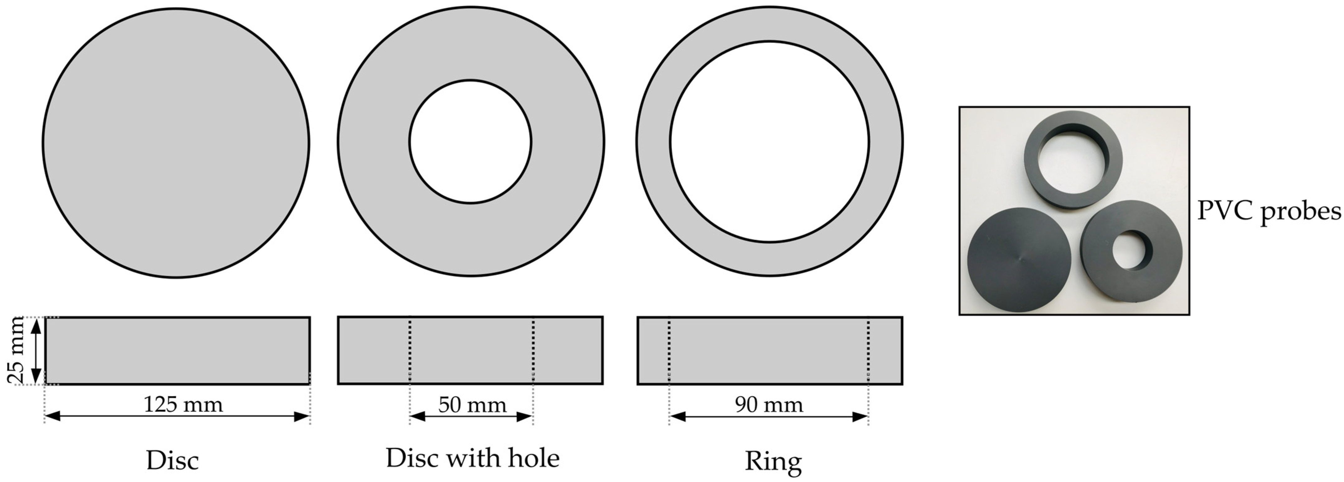
2.2. Sample Geometry

Sample geometries such as a disc, disc with a hole and ring are investigated in this study as shown in Figure 1. The outer probe diameter is fixed as 125 mm with a constant probe thickness of 25 mm. The inner diameter is varied from 0, 50 and 90 mm. These probe geometries are considered as the replacement geometries, for instance, a gear wheel in a real industrial application. The probes produced from plastic material (PVC) for cold experiments are also illustrated in Figure 1.

2.3. Experimental Setup with Measuring Techniques and Experimental Plan

In this study, three experimental setups are adopted as shown in Figure 2. In the utilized tubular suction wind tunnel with a diameter of 560 mm (Figure 2a), individual probes are examined. The plastic probes are fixed at the center of the tunnel inlet and the flow around the probes as well as the HTC on the probe surface are investigated within cold experiments. The cold experiment refers to the experiment in which the probes are not actually heated. Therefore, the probes for these experiments are of plastic material (PVC). Inside the model gas quenching chamber (Figure 2b) with chamber dimensions l × b × h = 970 × 650 × 1520 mm³, the flow field during quenching with batches is investigated by means of cold experiments. Plastic probes (PVC) are arranged in two layers and the flow behavior through and past the batches is examined. For the wind tunnel and the model chamber experiments, air at atmospheric pressure (1 atm) serves as the quenching fluid, where a ventilator controls the flow velocity. Figure 2c illustrates the Ipsen quenching plant with quenching chamber dimensions l × b × h = 625 × 435 × 420 mm³; here, the real quenching experiments with hot specimens are performed. The probe support frame for the batch has a dimension of 600 × 400 × 400 mm³. The experiments in the Ipsen plant are performed with the quenching gas N₂ with varied gas pressures. A maximum flow velocity (maximum ventilator power) is selected for all the quenching experiments, thus providing an average velocity of 13.4 m/s close to the inlet as measured at atmospheric conditions with air in a previous study [1].

Two-layered batches as depicted in Figure 3a are investigated with the Ipsen plant, where the probe-to-probe distance is fixed as 5 mm and the distance between the top and bottom layer is 35 mm. An additional space is provided below the second layer to accommodate the in situ temperature measurement/recording systems. Each probe within the batch is identified with a layer–row–column designation as shown in Figure 3b. For example, T-2-2 is identified as the probe from the top layer and positioned in the second row and second column. The temperature and cooling curves in some probes during batch quenching are measured in situ by means of thermocouples. Holes with a diameter of 1.1 mm (green markings in figure) in the specimen accommodate the thermocouples of diameter 1 mm (Figure 3c). The measurement locations T_core (core temperature), T_stag (staggered position temperature), and T_side (side/edge temperature) are at a depth of 12.5 mm, 16 mm, and 10 mm from the probe bottom surface. The thermocouples are held with support plates (Figure 3d). The temperature data are recorded by a data-logging system (Tpaq21/DATAPAQ) that is moving with the batch to the oven. More details of the experimental setups can be found in Refs. [1,2].

Different measurement techniques are adopted in this study to measure the flow velocity, convective heat transfer coefficient (HTC), and temperature of the probes during quenching. The pitot tube and 1D-CTA (constant temperature anemometry) probes shown in Figure 4a,b are adopted to measure the flow velocity. The HTC from the single-probe analysis is measured at different spatial positions of the probe surface by means of a glued-on film probe (DANTEC) (Figure 4c) [2,5,20]. A constant temperature of 100 °C is maintained in the film probe [21] by means of the CTA system. With the concept of a free jet calibration system, the wire and film probes are calibrated based on Equations (1)–(3) [3], valid in a range of 2.5 $\le$ r/D $\le$ 7.5, 2 $\le$ H/D $\le$ 12, and 2000 $\le$ Re $\le$ 400,000. The radial distance r is from the stagnation point, H is the distance between the plate and nozzle, D is the jet diameter (3.65 mm calibrator), Nu is the Nusselt number, Re is the jet Reynolds number, Pr is the Prandtl number, and $\lambda$ is the thermal conductivity of air. After calibrating the film probe on a perspex glass plate of 230 × 230 × 5 mm³, the film probe is carefully transferred to the probe surface and held on the surface by means of adhesive tape for measurement (Figure 4c).

$$\mathit{Nu}=\frac{\left[1-\frac{1.1D}{r}\right]}{\frac{r}{D}+\left[0.1\times \left[\frac{H}{D}-6\right]\right]}\times f\left(\mathit{Re}\right)\times {\mathit{Pr}}^{0.4}$$

(1)

$$f\left(\mathit{Re}\right)=2\times {\left[\mathit{Re}\times \left[1+0.005{\mathit{Re}}^{0.55}\right]\right]}^{0.5}$$

(2)

$$\mathit{HTC}=\frac{1-\frac{1.1D}{r}}{\frac{r}{D}+\left[0.1\times \left[\frac{H}{D}-6\right]\right]}\times f\left(\mathit{Re}\right)\times {\mathit{Pr}}^{0.4}\times \frac{\lambda }{D}$$

(3)

The 1D-CTA probe is implemented in the model chamber to measure the local flow field during the batch quenching. The batch is arranged in an inline or staggered fashion, where the 1D-CTA is fixed on the XY traversing stage. The flow field is measured; then, the probe is moved 10 mm and at each specific measurement point, the velocity is measured for 5 s with different frequencies as required. This XY positioning stage has a maximum movement range of 200 × 300 mm². The 1D-CTA measures continuously and a Python tool processes the data for obtaining the velocity contours.

During the heat treatment experiments (Figure 2c), the cooling curves are measured with a K-type thermocouple. The datalogger Datapaq-Tpaq21 [23] is used within the Ipsen plant for this purpose. The measurements are executed with a frequency of 3 Hz and a trigger temperature of 840 °C is initialized. The experimental plan of this study is concluded in

Table 1. Investigating parameters for suction wind tunnel and model chamber experiments.

Experimental Setup	Suction Wind Tunnel	Model Chamber
Probe	Disc	Disc, disc with hole, and ring
Material	Plastic (PVC)	Plastic (PVC)
Quenching fluid	Air at 1 atm	Air at 1 atm
Configuration	Single	Inline and staggered (Two layered)
Measurement	Flow velocity and HTC	Flow velocity/contour
Probe and measurement frequency	Film probe (100 Hz), 1D-CTA (500 Hz), pitot tube (1 Hz)	1D-CTA (1000 Hz)
Wire temperature (Twire)	100 °C	150 °C
Mean flow velocity (Vavg)	7.8, 9.8, and 12 m/s	2.5, 5.1, and 6.2 m/s
Distance between probes	Not applicable	5 mm
Distance between layers (supports) within the frame	Not applicable	50 mm

and

Table 2. Investigating parameters for quenching in Ipsen plant experiments.

Probes	Disc, disc with hole and ring
Material	42CrMo4 and 100Cr6
Quenching fluid	Nitrogen gas (N2)
Configuration	Inline/staggered—two layered
Measurement	Temperature
Furnace temperature (Tf)	850 °C
Gas pressure (P)	10 and 6 bar
Flow velocity (V)	13.4 m/s (2970 1/Min)
Furnace hold time (tf)	75 min
Measuring frequency	3 Hz
Distance between probes	5 mm
Distance between layers (supports) within the frame	35 mm

.

The heat-treated probes experience detailed hardness examinations. The sample hardness indentations for the probe geometries such as a disc, disc with a hole, and ring at the top and bottom sample surfaces can be observed in Figure 5. The local hardness has been measured in HRC by means of an automatic hardness testing machine (Hegewald & Peschke, Nossen, Germany).

3. Experimental Analysis

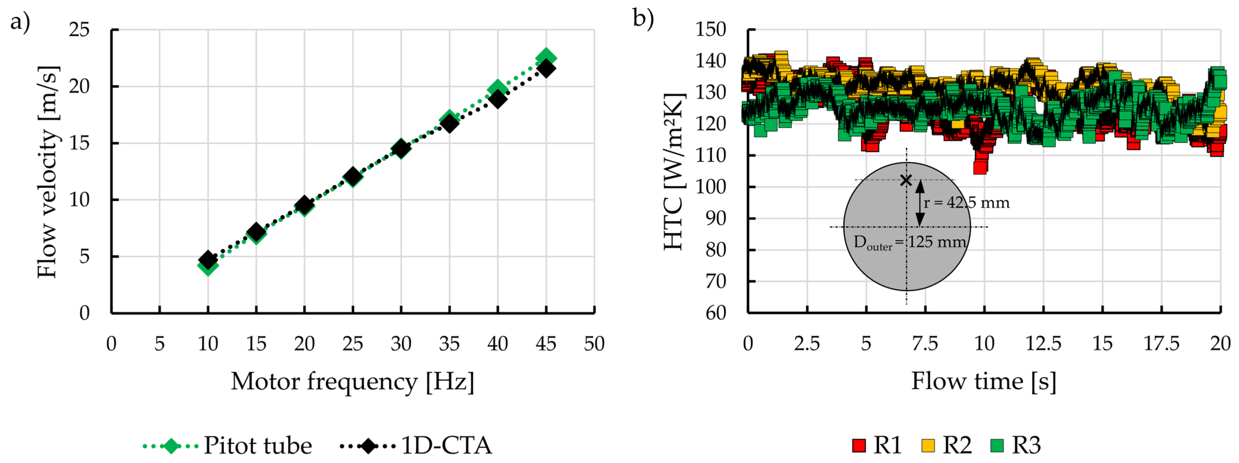
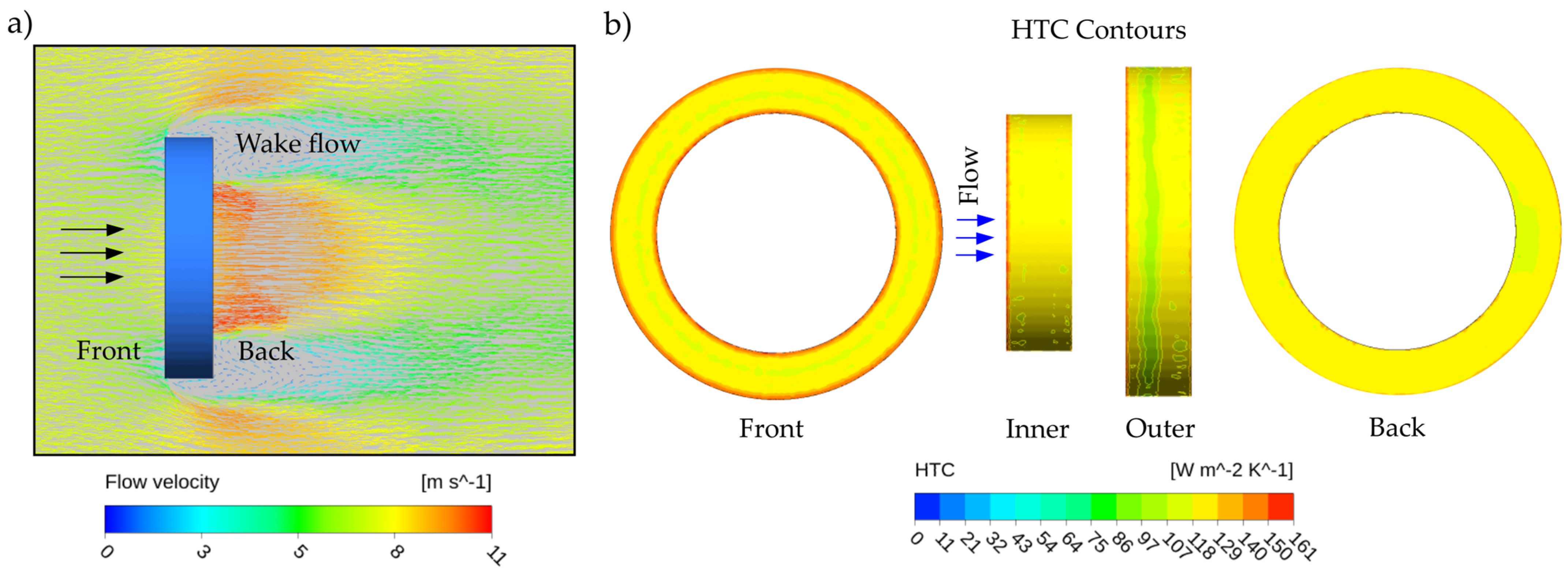
3.1. Determination of Flow Velocity and HTC in Wind Tunnel

Figure 6a shows the mean flow velocity at the center of the suction wind tunnel without any probe geometry and the motor frequency varies from 10 to 45 Hz. The measurements are carried out using pitot tubing (1 Hz) and 1D-CTA (500 Hz). The flow velocity almost linearly increases with the motor frequency. The two measurement techniques do not show much variation; however, a standard deviation of about 0.6 m/s is observed from 35 Hz onwards, which may be due to the increased turbulence.

The reproducibility of the HTC measurements within the wind tunnel has been verified with the disc probe. Therefore, the HTC measurements with the film probes at r = 42.5 mm (front side of disc probe) for a mean flow velocity of v = 7.8 m/s are consecutively measured three times for 20 s with a frequency of 100 Hz as depicted in Figure 6b. The results show that the measurements are repeatable with a standard deviation of 6.3 W/m²K.

Figure 7 shows the HTC measurements at two local positions at the disc for varying mean flow velocity with the parameters from Table 1. The radial position r = 42.5 mm normal to the flow field at the front of the probe and the local position at the circumference of the probe at half-thickness distance s = 12.5 mm from the front/back of the probe are selected for the HTC measurements. The HTC at the front of the probe especially near the probe edge is higher than at the circumferential position. From the stagnation point (r = 0), the flow deflects and accelerates towards the probe edge. This trend is also observed in [2,5] and the range of values (HTC) obtained is comparable. Moreover, the HTC increases with the flow velocity. This implies that the HTC is a function of probe geometry, local position and flow velocity.

3.2. Analysis of Flow Field within the Model Chamber

To investigate the influence of the flow field in batch quenching, experiments are performed with the quenching model chamber using the cold probes (non-heated) and with the process parameters from Table 1. Batch arrangements are constructed with discs, discs with a hole and ring samples. A sample batch arrangement with discs with a hole for an inline two-layered configuration can be seen in Figure 8b. This arrangement is similar to the one being investigated within heat treatment in the Ipsen plant. As the arrangement is symmetrical, the flow field for a measurement window of 200 × 300 mm² is investigated using the XY positioning stages and 1D-CTA (Figure 8c) and the flow measurements with batch samples are accomplished below the second layer (see Figure 8a,b).

An empty model chamber measurement is performed for three different gas flow rates based on ventilator frequencies 20, 30, and 40 Hz as shown in Figure 9a. The measurement plane is 130 mm above the top layer (compared to Figure 8b), considering this as the chamber inlet position resembling the Ipsen plant with a measurement sampling frequency of 1000 Hz. A higher measurement frequency is chosen to reduce the error [24]. The result shows that the maximum velocity (V_max) and average velocity (V_avg) increases with the flow rate resp. to ventilator frequency.

To investigate the influence of the batch arrangement on the flow field, three measurements are performed with the inline batch (two layered) of discs, discs with a hole and rings respectively, as seen in Figure 9b. The measurements are accomplished at a distance of 20 mm below the bottom layer (see Figure 8a,b) at a constant motor frequency of 30 Hz. It can be seen that the probe geometry within the batch has a significant impact on the flow field. The disc batch obtains a higher velocity in the gap area between the probes. This distribution is attributed due to the acceleration of the flow through the gaps between the probes. These higher and lower velocity fields indicate that the disc batch may have comparatively higher to lower HTC ranges during quenching. This can lead to uneven cooling within the probe. From these results, it can be expected that this accelerated flow through the gaps can increase the cooling effect on the following layers. Therefore, the bottom layer may cool faster than the top layer. Meanwhile, the disc with hole and ring batches do not have a very-high-velocity region as in the disc batch. This is because the flow splits into two streams, one part passing through the probe center and the second through the gap areas. As a result, the acceleration is comparatively lower than that of the disc batch. Comparing the disc with hole and ring batches, the disc with hole batch has a slightly accelerated region at the probe center and lower velocity fields below the probes. However, the batch with rings has a clear mixed trend, which indicates that the ring batch may possess uniform cooling action, and thereby a more uniform HTC distribution as well as quenching intensity is to be expected.

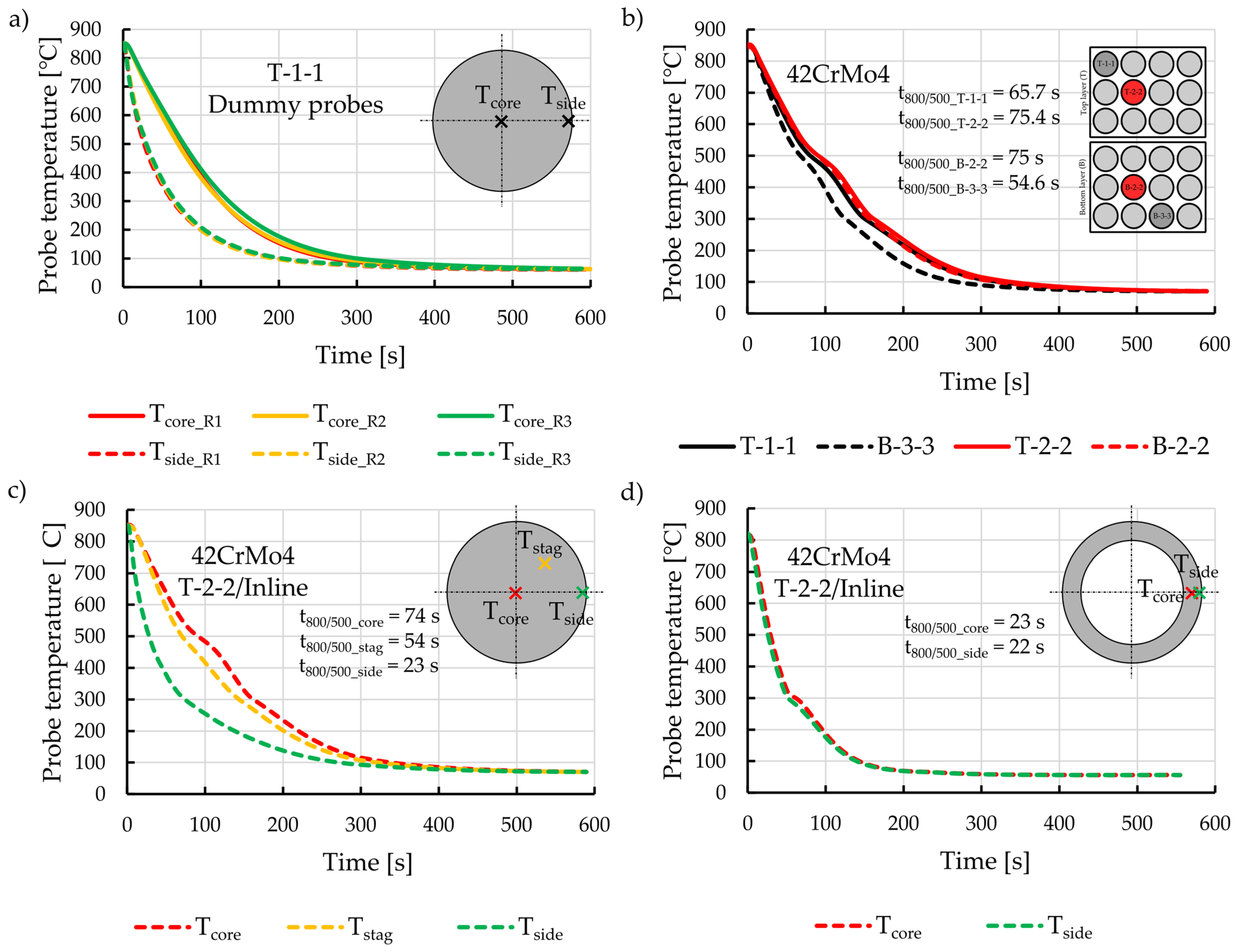
3.3. Quenching Trend within Batch and Probes

The temperature measurement reproducibility within heat treatment in the heat treatment facility (Ipsen plant) has been evaluated. Figure 10a depicts temperature measurement results from the core and side of the disc (austenitic) at position T-1-1 during 10-bar N₂ quenching with T_f = 850 °C and t_f = 75 min. The result shows that the measurements are reproducible with a maximum standard deviation of 19 °C.

Figure 10b depicts the 10 bar N₂ quenching trend within an inline disc batch of 42CrMo4 probes with T_f = 850 °C and t_f = 75 min. The outer and inner probes such as the T-1-1, T-2-2, B-2-2 and B-3-3 from the top and bottom layers are compared. The cooling curves depend on the probe location, i.e., even within a batch, different cooling intensities can be expected. In general, the outer probes cool faster than the inner probes in both layers. This is also expressed by the time t_800/500, which is the time required to quench a probe from 800 to 500 °C. The outer probes exhibit lower t_800/500. The outer probe from the bottom layer cools faster than the outer probe from the top layer. This is due to the accelerated flow from the top layer as discussed in Section 3.2 and Section 5.1.

In Figure 10c,d, the cooling trends for 42CrMo4 discs and rings during 10 bar N₂ quenching with T_f = 850 °C and t_f = 75 min are presented. Here, the discs show a higher cooling inhomogeneity, where the core is cooled slower than the side. Therefore, discs have a higher t_800/500 at the side, which decreases towards the inner core. This difference in cooling intensity can influence the microstructure constitution during quenching. Also, there are higher HTC resides at the edges of the discs, which is seen in the wind tunnel experiments (Section 3.1) and in CFD simulations (Section 5.1).

However, the ring probes have a more homogeneous cooling where a similar t_800/500 can be found at the side/edge as well as the core location. This implies that a homogeneous HTC distribution can be expected. In addition, the flow field analysis for the ring batch also showed an almost uniform flow field (Section 3.2). Therefore, a lower probe mass can lead to uniform quenching intensity within the probe volume.

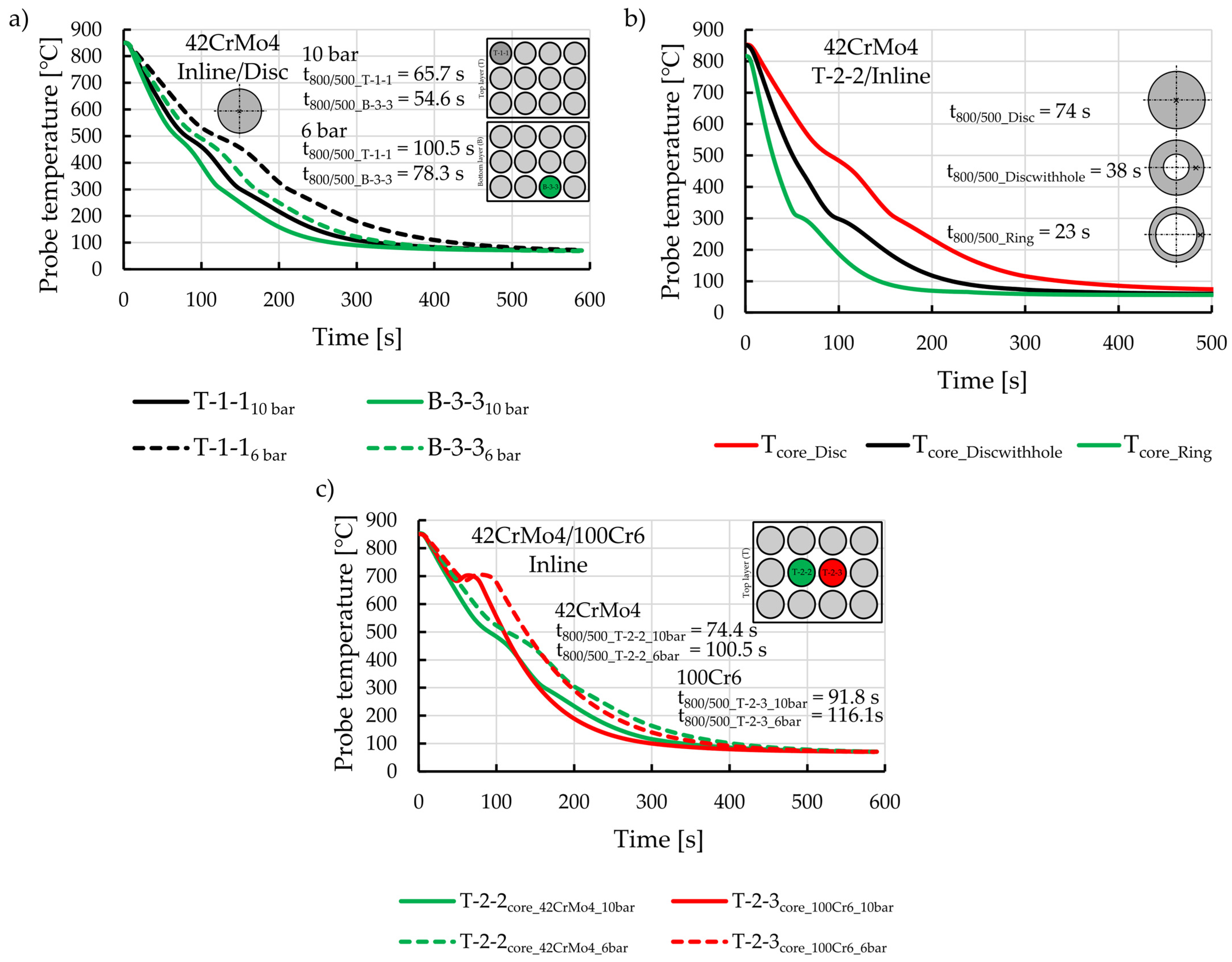
3.4. Influence of Gas Pressure, Probe Geometry, and Probe Material on Quenching

The influence of the gas pressure during N₂ quenching with T_f = 850 °C and t_f = 75 min is investigated. Therefore, the inline disc batch from 42CrMo4 is considered and the result is illustrated in Figure 11a. It can be seen that the 10 bar quenching is faster than the 6 bar quenching at the top and bottom layers, for which the 10 bar quenching has a smaller t_800/500 as observed in [1]. The increased gas pressure increases the gas density, and thereby the HTC. Therefore, in addition to the flow velocity, the increased gas pressure also contributes to the quenching intensity [1].

In Figure 11b, the quenching intensity for the different probe geometries is compared, considering 10 bar N₂ quenching of an inline batch at position T-2-2 with T_f = 850 °C and t_f = 75 min. The probe with lower mass cools down faster and has a lower t_800/500, indicating that the probe geometry/probe mass has a significant role in the quenching intensity.

To evaluate the influence of the probe materials on quenching, the 10 bar N₂ quenching is performed on 42CrMo4 and 100Cr6 probes at position T-2-2 and T-2-3 within an inline disc batch (T_f = 850 °C, t_f = 75 min), which are the directly comparable symmetrical positions as in Figure 11c. The result indicates that the material type also influences the cooling curve, where the 100Cr6 is cooled more slowly than the 42CrMo4. The thermal diffusivity of 100Cr6 is lower and more latent heat is released from 100Cr6 during material transformation. This implies that the material type should also be considered during batch quenching.

In order to compare all the heat treatment experiments (Ipsen plant) and to evaluate the batches, the minimum, maximum and average cooling rates from all the experiments are summarized in

Table 3. Minimum, maximum and average cooling rates for batch quenching (Ipsen plant experiments).

Sl. No	Probe	Configuration	Pressure (bar) Vavg = 13.4 m/s	Minimum Cooling Rate from Batch (°C/s)	Maximum Cooling Rate from Batch (°C/s)	Average Cooling Rate from Batch (°C/s)
1	Disc	Inline	10	4	5.49	4.52
2	Disc	Staggered	10	4.33	5.41	4.68
3	Disc	Inline	6	2.99	3.83	3.30
4	Disc with hole	Inline	10	7.32	9.09	8.05
5	Disc with hole	Staggered	10	8.47	9.52	8.96
6	Disc with hole	Inline	6	5.95	7.25	6.51
7	Ring	Inline	10	11.54	13.64	12.68
8	Ring	Staggered	10	11.76	14.49	12.89
9	Ring	Inline	6	7.94	10.99	9.55

. The batch with rings (lower probe mass) has a significantly higher cooling rate and this decreases towards the probe disc (with higher probe mass). The average cooling rate is higher for the staggered configuration from all the investigated batch cases as well as the cooling rate decreases with the lower gas pressure. In the staggered configuration, the accelerated flow through the gaps from the top layer contributes towards a higher HTC at the bottom layer and thereby the cooling rate.

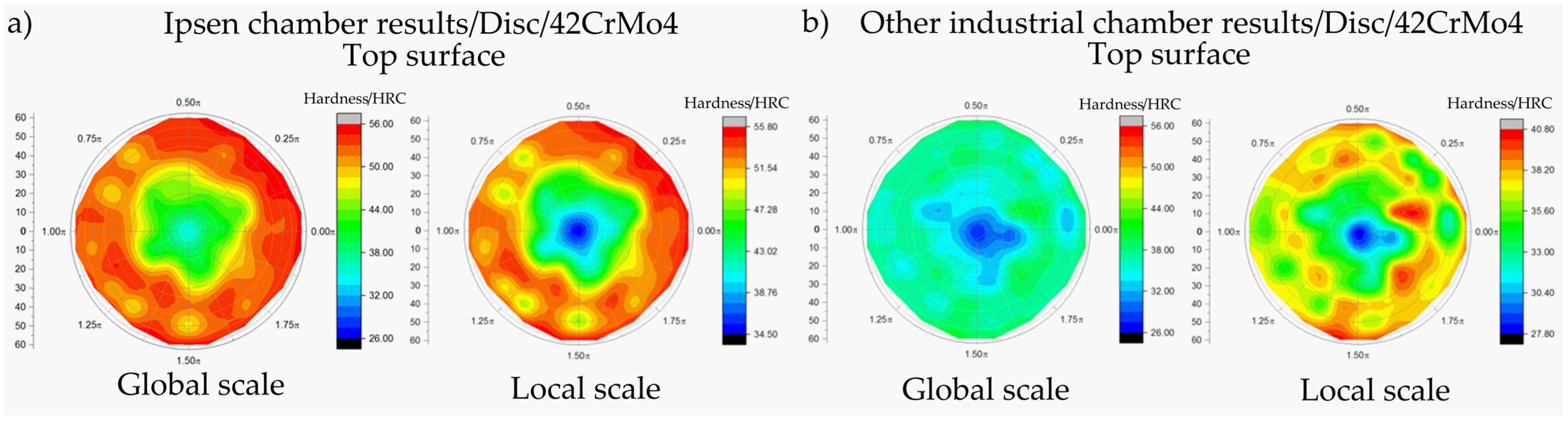
3.5. Influence of Quenching Parameters on Material Hardness

Selected hardness results are shown in Figure 12a,b for the discs and in Figure 12c,d for the rings, comparing 10 bar and 6 bar quenching. For easier comparability of the hardness values, the scaling of the hardness is between 20 and 65 HRC. The hardness correlates with the observed microstructures. The hardness differences between the top and bottom sides are minor. The hardness increases towards the edge of the sample. This behavior correlates with the increasing martensite content towards the edge. The hardness is lowest at the center of the samples in agreement with the results of the temperature investigations. The influence of the gas pressure indicates that with decreasing gas pressure, the cooling rate of the sample decreases and lower hardness is attained. The differences between the inline and the staggered arrangement are not significant. With decreasing probe volume/mass, the hardness distribution is more homogeneous within the probe, i.e., the hardness variation between the edge and the center of the probe is small. With decreasing probe volume (mass), the cooling rate increases so that the critical cooling rate is reached for larger volume areas of the probe. The results of the surface hardness can also be transferred to the hardness levels in the cross-sections. Thus, with increasing specimen volume, the differences between the edge and core increase (comparison of disc and ring samples in Figure 12). The differences between a gas pressure of 6 bar and 10 bar and the differences between 42CrMo4 and 100Cr6 are also confirmed.

4. Numerical Modeling (CFD, FEM) and Artificial Neural Networking (ANN)

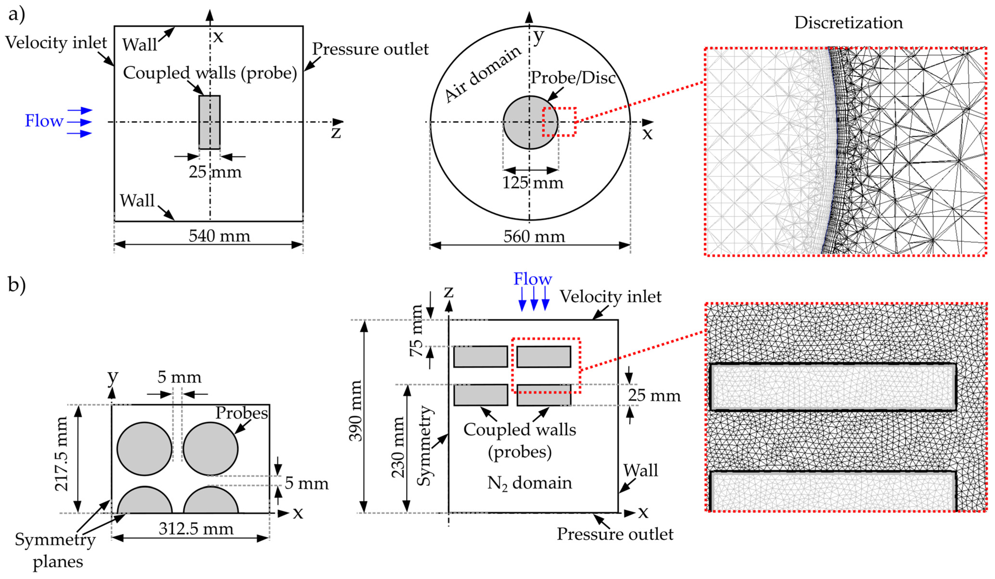
4.1. Computational Fluid Dynamics (CFD)

To perform the numerical simulations (CFD), the domain representing the wind tunnel and the furnace with batches (resembling the Ipsen batch) geometries is created and spatially discretized in ANSYS ICEM-CFD 19.2 [25] as depicted in Figure 13. Figure 13a shows the full 3D-computational domain and the corresponding discretization for the single-probe simulation. In this case, a velocity inlet and pressure outlet are implemented as well as the specimen surface being defined as a coupled wall for this conjugate heat transfer process. In addition, fine cells (prism layers) are provided in the boundary layer close to the probe surface for improving the results.

Figure 13b illustrates the computational domain together with the discretization for an inline batch consisting of discs. Here, only one quadrant is modeled due to the symmetry of the domain. A flow inlet and pressure outlet are modeled as in the single-probe simulation and the specimen surfaces are implemented as coupled walls. Correspondingly, different batches such as the inline and the staggered with different probe geometries are created for the numerical simulations. However, the simulations show that the results are mesh-dependent. Therefore, considering the single-probe wind tunnel experiments, a suitable first cell height near a wall for the single-probe simulation has been identified as 0.5 mm and for the batch quenching as 0.25 mm, provided for five layers. If the cell height close to a near-wall region is further reduced, the HTC is significantly overpredicted. The reliability of this selected near-wall cell height for batch quenching is again verified in Section 5.3 (Figure 21c). The single probe and the batch mesh have approximately 1 × 10⁶ and 3 × 10⁶ computational cells, respectively.

The HTC in gas quenching does not change significantly with time [1]. Therefore, the numerical simulations (CFD) are modeled as stationary. The probe material is 42CrMo4 in the simulation and the material properties required for simulation are taken from the supplier manual for 20 °C, i.e., the thermal conductivity of 42.6 W/(m·K), density of 7720 Kg/m³, and heat capacity of 470 J/(Kg·K). The gas properties of air at 1 bar and nitrogen N₂ at 10, 8 and 6 bar are adopted from [3] at 70 °C, since the average gas temperature during quenching has been measured as 70 °C. The stationary simulation is modeled in ANSYS Fluent 19.2 [26] and the pressure–velocity-coupling SIMPLE and the turbulence model kω-SST model have been adopted, as the kω-SST turbulence model provides a better combination for wall proximity and for the mean flow [27].

The CFD simulations with the single probes and the batches together with the simulation parameters are concluded in

Table 4. Parameters for single-probe CFD simulation.

Probes	Disc, Ring
Material	42CrMo4
Quenching fluid	Air
Pressure (bar)	1
Flow velocity (m/s)	7.8, 9.8, and 12
Probe temperature (Tprobe)	100 °C (373.15 K)
Air temperature (Tair)	18 °C (291.15 K)

and

Table 5. Parameters for CFD batch simulations.

Probes	Disc, disc with hole, and ring
Configuration	Inline and staggered (two layered)
Material	42CrMo4
Quenching fluid	Nitrogen gas (N2)
Pressure (bar)	6, 8 and 10
Flow velocity (m/s)	8, 10 and 13.4
Probe temperature (Tprobe)	850 °C (1123.15 K)
Gas temperature (TN2)	70 °C (343.15 K)

.

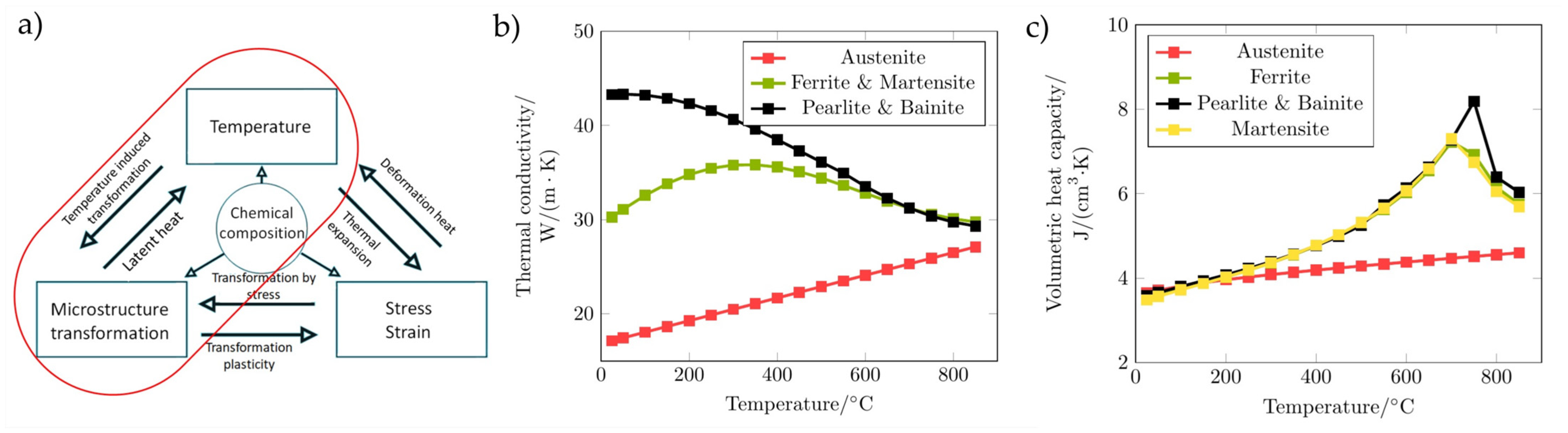
4.2. Finite Element Method (FEM)

By means of FEM computations, it is possible to map the development of the microstructure and hardness of the heat-treated probes depending on the boundary conditions, which are determined from the CFD simulations described above. The boundary conditions can vary depending on the local position. The calculation of the temperature evolution is based on the heat conduction equation (Equation (4)) [28]. The heat conduction equation enables the consideration of the thermal conductivity, the specific heat capacity, the density and transformation processes. The heat capacity and the density result in the volumetric heat capacity. In Equation (4), $\rho$ is the density, $c\left(\vartheta \right)$ and $\lambda \left(\vartheta \right)$ are the temperature-dependent specific heat capacity and thermal conductivity, $\vartheta$ is the temperature, $\dot{W}$ is the power density (energy released from phase transformation), $x$ is the position, and $t$ is the time.

$$\rho c\left(\vartheta \right)\frac{\partial \vartheta }{\partial t}=\mathit{div}\left[\lambda \left(\vartheta \right)\mathit{grad}\left(\vartheta \right)\right]+\dot{W}(\vartheta ,x,t)$$

(4)

The transformation processes are represented by isothermal time–temperature–transformation (TTT) diagrams, taking into account the latent heat. The relationships of the microstructure and hardness simulations are shown in Figure 14a based on [29,30]. It can be seen that there are interactions between the development of the temperature and the microstructure due to the latent heat release, the temperature-induced transformation, etc. This trend also illustrates the necessity to model the material characteristics as a function of temperature and microstructure. Furthermore, in addition to the development of the temperature and the microstructure, the FEM simulations also allow the stresses and strains arising from the heat treatment to be taken into account. Thus, it is possible to calculate residual stresses and the distortion of the components and illustrate the potential of simulations that take into account the microstructure transformations during heat treatments. The steel material parameters used for the numerical computations are calculated using JMatPro V7.0 as a function of the chemical composition. JMatPro is a tool for calculating the temperature-dependent material properties for a variety of technical alloys [31]. The material properties can be determined as a function of the various microstructural constituents, so-called “mixture material”. The microstructural constituents taken into account for the steels under investigation are austenite, ferrite/pearlite, bainite and martensite. In addition, transformation data, in particular isothermal TTT, can be generated using JMatPro. The calculated material data are compared with other characteristic values from databases, the literature, and experimental investigations (i.e., hardness, dilatometry, and calorimetry). Selected material data are shown as an example for 42CrMo4 (AISI4140) in Figure 14b,c.

The FEM simulation model has been solved using Deform-HT using 2D and 3D models. The consideration of transformation is implemented by using isothermal transformation data, i.e., input of start and end curves of transformations is required. The evolution of the microstructure is calculated based on the JMAK equation [30], see Equation (5), where the $\xi$ is the volumetric phase transformed, t is the time, and k and n are constants. By using an additivity rule [30,32] and the transfer to the geometry by meshing (FE), varying continuous cooling curves can be calculated. If the respective local volume fractions of the microstructural constituents are known, the local hardness (HV) can be calculated based on the mixing rule, see Equation (6), where V_M, V_B, V_P, V_F, and V_A are the respective volume fractions of microstructural constituents such as martensite, bainite, pearlite, ferrite, and austenite; the H_M, H_B, H_P, H_F, and H_A are the corresponding hardnesses. As seen in Equation (6), the mixing rule requires the input of the hardnesses of the individual microstructural constituents. The total sum of the volume fraction remains at 100% as in Equation (7). The hardnesses are determined using JMatPro (see

Table 6. Hardness values calculated from continuous cooling transformation (CCT) phase diagram data with JMatPro using optimization algorithms in Matlab (lower limit = 10 HRC assumed).

42CrMo4 (AISI4140)	Hardness/HRC
Austenite/Ferrite	10
Pearlite	20
Bainite	42
Martensite	60

) and/or experimentally. The hardness of individual microstructural constituents of the steel has been measured by means of Martens hardness and HV1/HV10, among others. The comparison of the calculated and experimentally determined hardness shows good agreement. It should be noted that numerical simulations should be validated, in particular if calculated material parameters or material parameters from the literature are used for the various material models. This can be performed in the area of the simulation of microstructural developments, for example, by means of dilatometry tests, the Jominy end quench test, or also thermally treated components in which the development of the temperature has been measured [29].

$$\xi =1-\mathit{exp}(-k·t^n)$$

(5)

$${\mathit{HV}}_{\mathit{total}}=\frac{H_M·V_M+H_B·V_B+H_P·V_P+H_F·V_F+H_A·V_A}{100\%}$$

(6)

$$V_M+V_B+V_P+V_F+V_A=100\%$$

(7)

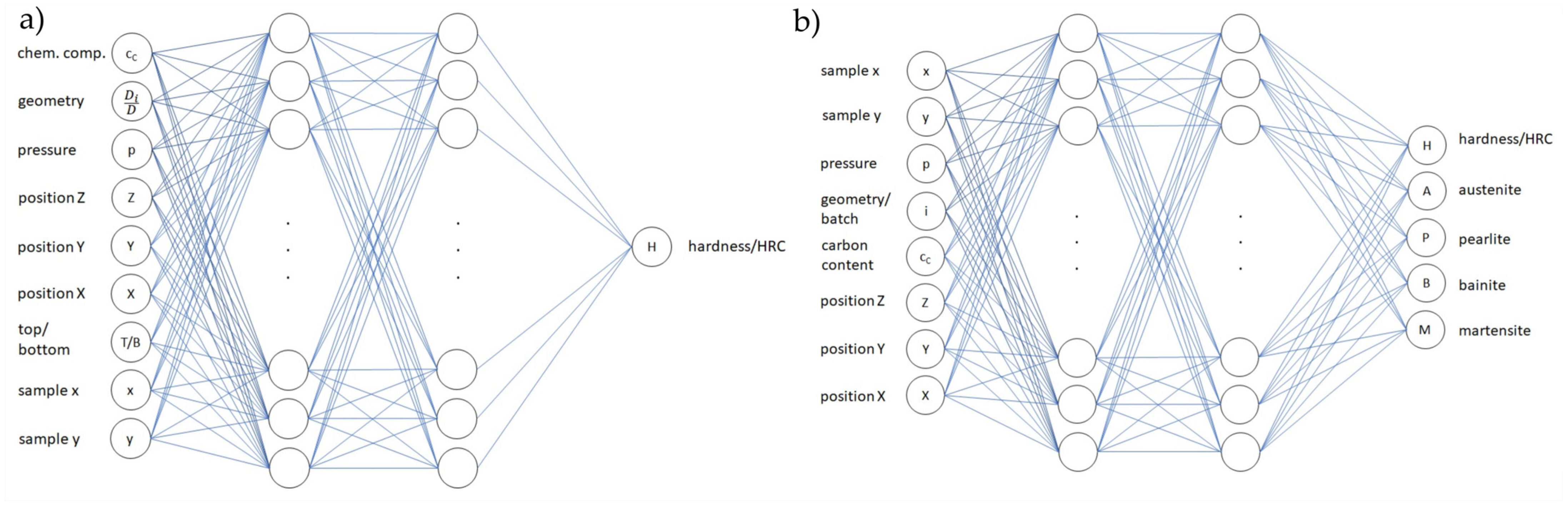
4.3. Artificial Neural Network (ANN)

The MATLAB (MATrix LABoratory) software package version R2016b (MathWorks company) is used to create and train the ANN (artificial neural network). The number of neurons and hidden layers as well as the transfer functions (logsig, tansig, purelin) and the training algorithms (Levenberg–Marquardt and Bayesian Regularization) can be varied. Inputs included various parameters such as chemical composition by carbon content, location within the batch, local coordinates x and y of the probe, front/back of the probe, geometry by using the quotient of the inner diameter and outer diameter of the metal probes (Di/D), quenching pressure and ventilator speed of the quenching process. The data sets were each split into 60% for training, 20% for validation and 20% as test data, i.e., the unseen data.

Since the measurement of hardness using HRC made it possible to perform a high number of hardness measurements and thus generate many measurement/data points, an ANN has been trained using the experimentally determined hardness measurement values as output. The structure of this ANN is shown schematically in Figure 15a. The input data used for training the ANN include 10,774 data points, i.e., approximately 56 samples each with a top/bottom. In total, 60% of the data have been used for training, 20% for validation, and 20% as test data, i.e., the unseen data.

The results of the FEM simulations, which are based on the CFD data (average surface HTC), were also transferred to an ANN (see Figure 24). The data used for this ANN have been modeled in 2D at the initial stage, so that the cross-section of the sample could be mapped rotationally and symmetrically. It should be noted that 3D modeling with the locally varying HTC around the plane of rotation will lead to a further improvement in the results. The schematic structure of the ANN is shown in Figure 15b. In addition to the hardness values, other output variables, such as the respective volume fractions, are calculated. The advantage of this method using CFD and FEM is that a large number of data points can be generated, where several parameter variations can be performed “virtually” and also within the specimens, “virtual” measurements can be performed experimentally at the hard-to-reach locations. The input data used for the training of the ANN are based on the FEM simulations and comprise about 12,000 data points. Again, 60% of the data were used for training, 20% for validation and 20% as test data, i.e., the unseen data.

5. Discussion of Simulation Results

5.1. Validation of Numerical Model (CFD) and Numerical Results

The numerical model (CFD) is validated with the experimental results based on the wind tunnel results. To accomplish this, the simulation case similar to the wind tunnel experiment in Section 3.1 with the disc is set up where the mean flow velocity V_avg = 7.8 m/s, the probe temperature T_probe = 100 °C and air temperature T_air = 18 °C with 42CrMo4 material.

Figure 16a shows the HTC distribution from the surfaces as a function of the distance along with the HTC contours. The HTC increases towards the edge of the probe as seen in the experiments (Section 3.1 and Section 3.4). The front and back edges have comparably higher HTC, whereas the stagnation zone has lower HTC. Towards the edge of the probe, the flow accelerates after deflecting from the stagnation region as shown in the velocity vector in Figure 16b. The accelerated flow towards the probe edge contributes to higher HTC. Moreover, behind the probe, a wake zone is seen as observed in [2]. The lower velocity at the stagnation region leads to a lower HTC region at the probe center; behind the probe, a more uniform HTC distribution is observed. The measurement results from the front and circumference locations are compared with the numerical results. The front HTC is in reasonable agreement (deviation of 6.5%) with the experimental result. However, the circumferential HTC has some deviation from the experiment. This may be due to the reason that, at the circumferential region, some recirculation is seen (Figure 16b), and thereby the film probe is not ideally capable of detecting this and is deviating from the calibration configuration. The obtained HTC ranges are comparable with the previous studies for the single-probe quenching in the 1 atm condition and higher HTC is observed at the probe edges and corners [2,5].

The influence of the flow velocity is investigated by varying the flow velocity to 7.8, 9.8 and 12 m/s as shown in Figure 16c for the disc probe. As observed earlier in the wind tunnel experiments (Section 3.1), the HTC increases with increased flow velocity and the probe edge possesses higher HTC.

To investigate the influence of the probe geometry, the ring probe is further simulated under the same conditions as with the disc. The results are depicted in Figure 17. The velocity vector in Figure 17a shows that the mean flow splits into two streams, one stream flowing through the probe center and the other through the probe outer surface. Two local wake flows are observed around the circumference region towards the probe rear surface. The HTC contours in Figure 17b illustrate that the front and back edges possess higher HTC and the surfaces with more or less a uniform HTC distribution. This trend points out that the cooling of rings may be homogeneous.

In the batch simulation (Table 5), the flow velocity at the inlet is taken as V = 13.4 m/s, which has been determined in previous research [1]. However, before proceeding to the series of batch simulations, a reverse engineering approach has been adopted to verify the reliability of the HTC computed by the batch simulation (CFD) with the near-wall cell sizes. For this purpose, the experimentally determined core temperature over time for the probe T-2-2 (42CrMo4) for the inline arrangement of disc, disc with hole, and ring batch quenching with T_probe = 850 °C during 10 bar N₂ gas quenching is compared to the core temperature evolution determined by the FEM model. This has been modeled based on the HTC values computed by the CFD batch simulation. The result is shown in Figure 21c (Section 5.3) and shows good agreement, confirming that the HTC computed by the CFD simulation can be reliably implemented into the FEM simulations.

From the series of batch simulations (Table 5), some representative results are presented in Figure 18. In Figure 18a,b, the HTC contours and velocity vectors from the inline disc and ring batches during 10 bar N₂ quenching with T_probe = 850 °C and V = 13.4 m/s are presented. Comparing the single-probe results (Figure 16a), the HTC distributions for the batches are asymmetric particularly for the discs. This is due to the complex flow fields emerging from the batch and from the flow acceleration through gaps and interactions as observed in the flow field analysis (Section 3.2). The flow acceleration through the gap between the discs and the flow splitting with the ring probes are clearly visible from the velocity vectors. Due to the flow acceleration (nozzle effect), the bottom probes exhibit a higher HTC than the top layer. This shows why the bottom probes cooled faster in the batch experiments (Figure 10b). With the ring batch, the top layer has more or less symmetrical behavior but the flow splitting and turbulent interactions towards the bottom layer leaves behind an asymmetric HTC distribution at the bottom layer. While comparing the maximum velocity from the batches, the disc batch possesses higher (maximum) velocity for the flow as observed in the flow field analysis (Section 3.2). Due to this higher flow velocity, the disc batch attained higher HTC. In Figure 18c, the HTC contours and velocity vectors from the staggered disc batch during 10 bar N₂ quenching with T_probe = 850 °C and V = 13.4 m/s are presented. Compared with the inline batch (Figure 18a), the bottom layer of the staggered batch possesses higher HTC. This is because the flow accelerated through the gap region from the top layer is directed to the probes at the bottom layer, and thereby the heat transfer is significantly improved. The HTC as well as the heat transfer performance are better for the staggered configuration as observed in the batch heat treatment experiments (Section 3.4, Table 3). In addition, the HTC distributions (top layer) obtained from the CFD simulations (Figure 18) can also be compared qualitatively with the hardness measurements from the probes, Figure 12a,b. The higher HTC regions at the disc probe result in improved hardness whereas for the rings, more or less uniform HTC is observed, and thereby uniform hardness.

The influence of the flow velocity and the gas pressure on the HTC within the batch quenching has been investigated. For this, the probe T-2-2 (42CrMo4) from the inline disc batch during N₂ quenching with T_probe = 850 °C is considered and the results are presented in Figure 19a,b. The higher flow velocity and the gas pressure have a positive impact on the HTC distribution. This means that in the gas quenching process, the gas pressure and the flow velocity can be considered as the main important process control parameters that determine the quenching intensity as observed in [1,2].

The minimum and maximum HTCs obtained from the numerical simulations of the batches are summarized in

Table 7. Minimum and maximum HTC from the CFD batch simulation for the batch arrangements from Table 5.

Sl. No	Probe	Configuration	Gas Pressure (Bar)	Flow Velocity (m/s)	Minimum HTC from Batch (W/m2K)	Maximum HTC from Batch (W/m2K)
1	Disc	Inline	10	13.4	357	2103
2	Disc	Staggered	10	13.4	393	2563
3	Disc	Inline	10	10	284	1670
4	Disc	Inline	10	8	240	1378
5	Disc	Inline	8	13.4	299	1749
6	Disc	Inline	6	13.4	210	1208
7	Disc with hole	Inline	10	13.4	279	1776
8	Disc with hole	Staggered	10	13.4	310	2016
9	Disc with hole	Inline	8	13.4	229	1481
10	Disc with hole	Inline	6	13.4	155	1037
11	Ring	Inline	10	13.4	318	1289
12	Ring	Staggered	10	13.4	307	1440
13	Ring	Inline	10	10	251	1013
14	Ring	Inline	10	8	210	910
15	Ring	Inline	8	13.4	264	1065
16	Ring	Inline	6	13.4	182	809

. The staggered configuration generally performs better, providing a higher HTC. By increasing either the gas pressure or the flow velocity, the minimum and maximum HTC range with the batch quenching can be adjusted. The HTC ranges obtained from this high-pressure quenching with N₂ in this study (Table 7) are comparable with a previous study [1], in which for a flow velocity of about 7 m/s with 10-bar N₂ quenching for batches with cylindrical probes, a maximum HTC of order 1000 W/m²K has been observed. Similar HTC ranges are also observed in [4,33]; however, the geometries are not directly comparable.

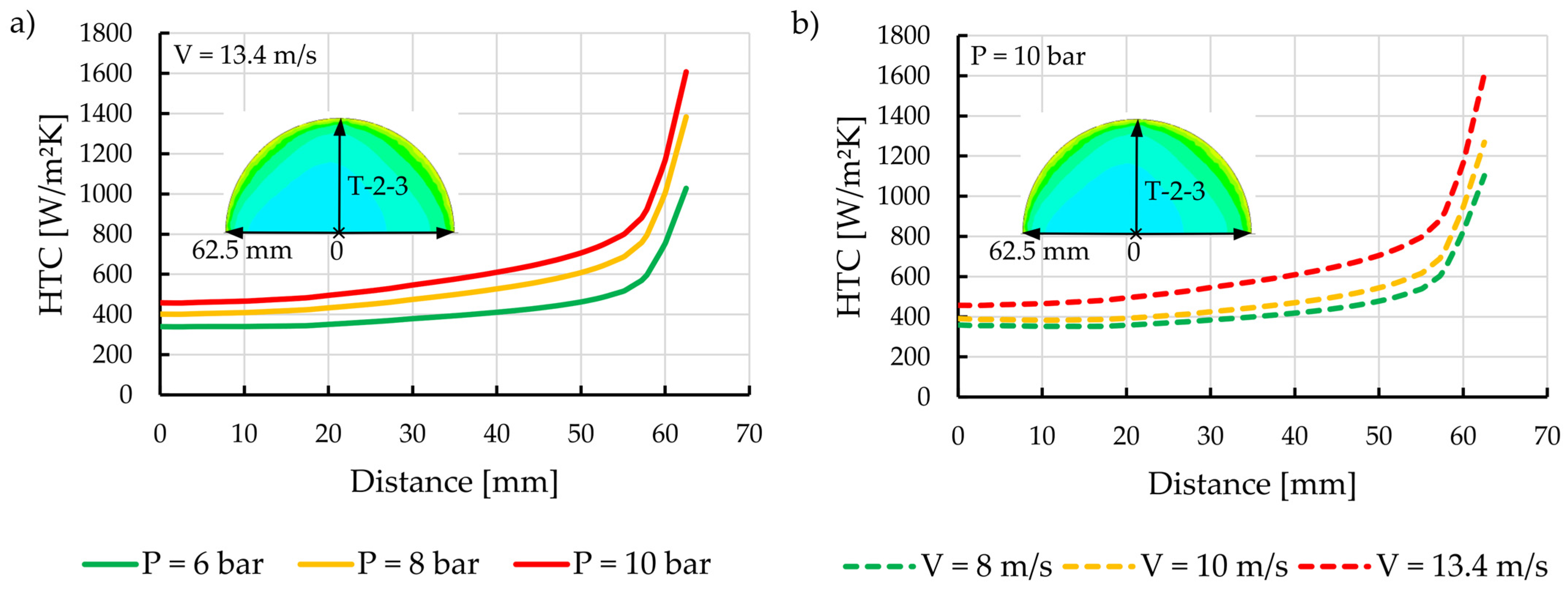
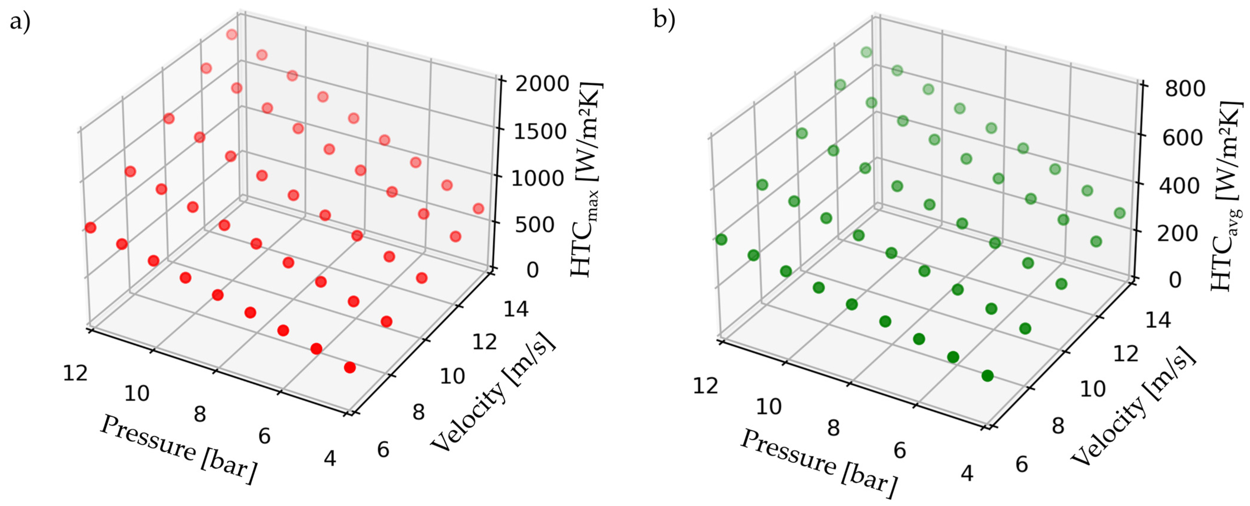
5.2. Correlation for HTC

The local HTC is a function of probe geometry, local position on the probe surface, flow velocity and gas pressure, i.e., HTC = f (geometry, radius, flow velocity, gas pressure). Typical HTC correlations are based on Re (Reynolds number) and Pr (Prandtl number), thus implying the relationship with flow velocity and gas pressure [1].

Therefore, in order to mathematically illustrate the effect of flow velocity and the gas pressure on the HTC for the N₂ gas quenching of inline disc batches (42CrMo4) with T_probe = 850 °C, a power law function is considered based on the effect of single parameters on HTC. As an example, the average surface HTC from the probe position T-2-2/T-2-3 over the radius at the probe top surface is selected from all the simulation results. The correlation for the maximum HTC (HTC_max) and average HTC (HTC_avg) over the radius is correlated by using a data fitting algorithm (python code/scipy.optimize.curve_fit based on non-linear least squares) and presented in Equations (8) and (9), where P is gas pressure in bar and V is mean flow velocity at the inlet in m/s. This correlation is developed for the velocity range 8 to 13.4 m/s and for the gas pressure range 6 to 10 bar for N₂ quenching at 850 °C. The correlations deviate by 4% from the simulation results for the 42CrMo4.

$${\mathit{HTC}}_{\mathit{max}}\left(T-2-3\right)=31.96\times P^{0.84}\times V^{0.77}$$

(8)

$${\mathit{HTC}}_{\mathit{avg}}(T-2-3)=18.59\times P^{0.72}\times V^{0.71}$$

(9)

Even though Equations (8) and (9) are determined for the above-mentioned velocity and gas pressure ranges only, an extrapolation to outside the range is to be briefly examined. Since the densities of nitrogen N₂ and air at ambient pressure are almost identical, the maximum HTC (HTC_max) with Equation (8) for a gas pressure of P = 1 bar and velocity of V = 7.8, 9.8 and 12 m/s (similar to the single-probe simulation; Section 3.1, Figure 7) is computed as 155.4, 185.2, and 216.5 W/(m²·K), which is in an acceptable range when compared with the single-disc CFD investigation (Figure 16c). Therefore, HTC values at velocities from 6 to 14 m/s and gas pressure from 4 to 12 bar are presented based on the correlations, Equations (8) and (9), in Figure 20a,b. The increasing trend of the HTC based on flow velocity and gas pressure can be observed.

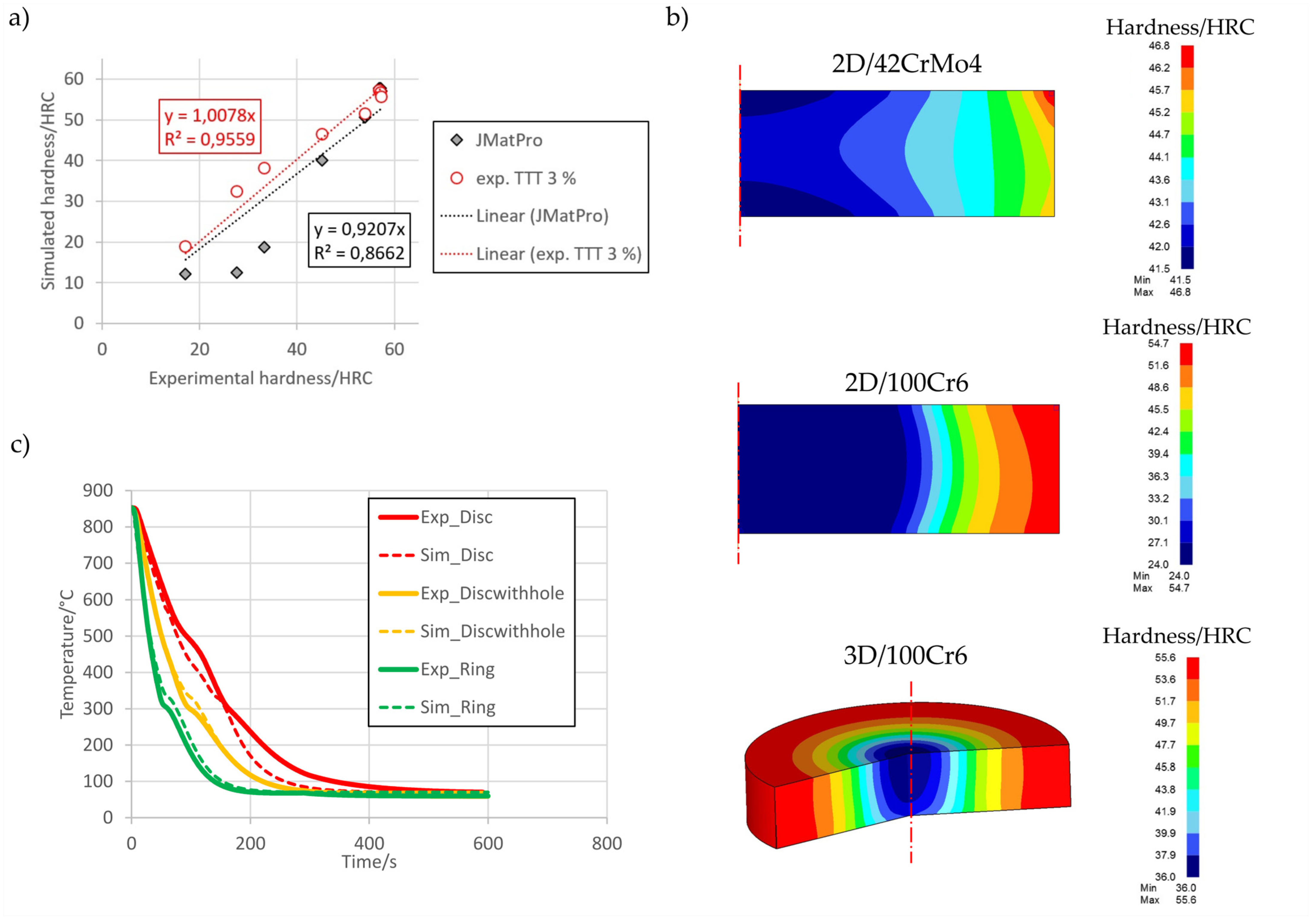
5.3. Results from FEM Modeling

The validation of the FEM simulations has been carried out on dilatometer tests, e.g., continuous cooling tests. The advantage is that the temperature is known and a homogeneous temperature field over the entire specimen can be assumed for simplicity. This allows the comparison of the resulting microstructural constituents and hardness as a function of the different cooling rates. The simulation results show good agreement with the experiments; see Figure 21a. For the further calculations, the material model has been adopted with the calculated JMatPro data, supplemented by the experimentally determined TTT (exp. TTT).

Based on the validation data, the transformation data (TTT) in particular exert a major influence on the simulation results of the microstructure and hardness development. In Figure 21a, the transformation data based on JMatPro for the 42CrMo4 illustrate a slightly higher deviation in the example shown. It should be noted that this may also be due to a deviation in the input data required for the JMatPro calculations (chemical composition, grain size, etc.). This trend illustrates that the transformation data from calculation tools, a database, or the literature can be used, but should always be checked with validation experiments, such as the dilatometer test presented here. For the further calculations, the material model with the experimentally determined isothermal TTT was used (exp. TTT).

The results obtained underline that the position of the specimens and the batch arrangement influence the local heat transfer coefficient (HTC) and thus the respective cooling behavior. The influence of the batch and the influence of the location positions are possible by considering the boundary conditions calculated by CFD in the FEM calculations. These local HTCs have been transferred element by element to the FEM boundary conditions. Selected results of the FEM simulations are shown in Figure 21b. The consideration of the heterogeneous local HTC affects the calculated hardness.

The respective temperature evolution from the FEM simulations from the sample core with boundary conditions based on the CFD data (surface HTC) is compared with the temperature evolution of the sample core from the heat treatment experiments (Ipsen) with T_f = 850 °C and 10 bar N₂ quenching for probe position T-2-2 (42CrMo4) in Figure 21c. Smaller deviations can be seen in the area of phase transformations, which can be attributed to slightly different latent heat released. The latent heat values taken into account in the FEM simulation are based on calculated material parameters from JMATPro. Moreover, constant material properties are considered in the CFD stationary simulations.

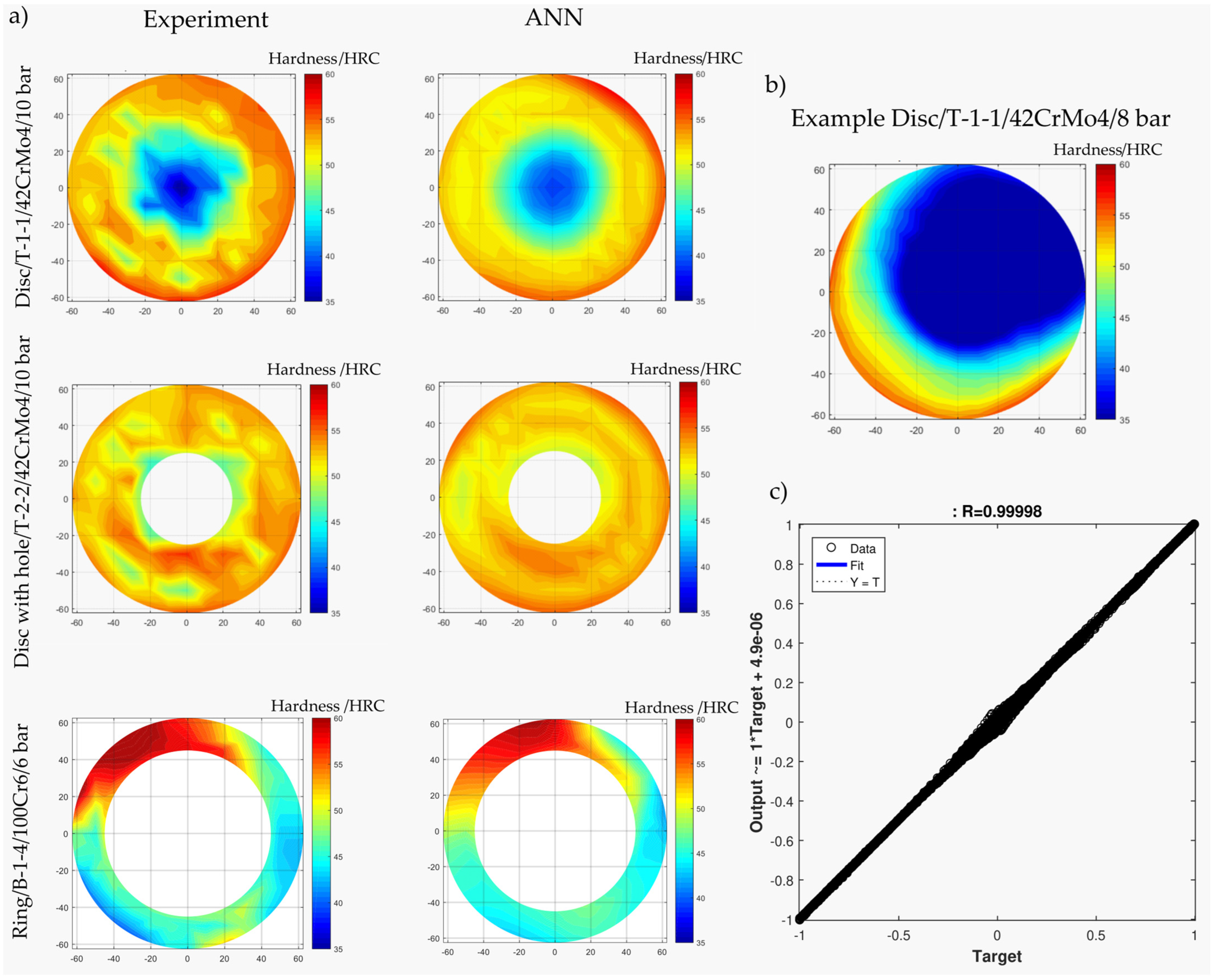
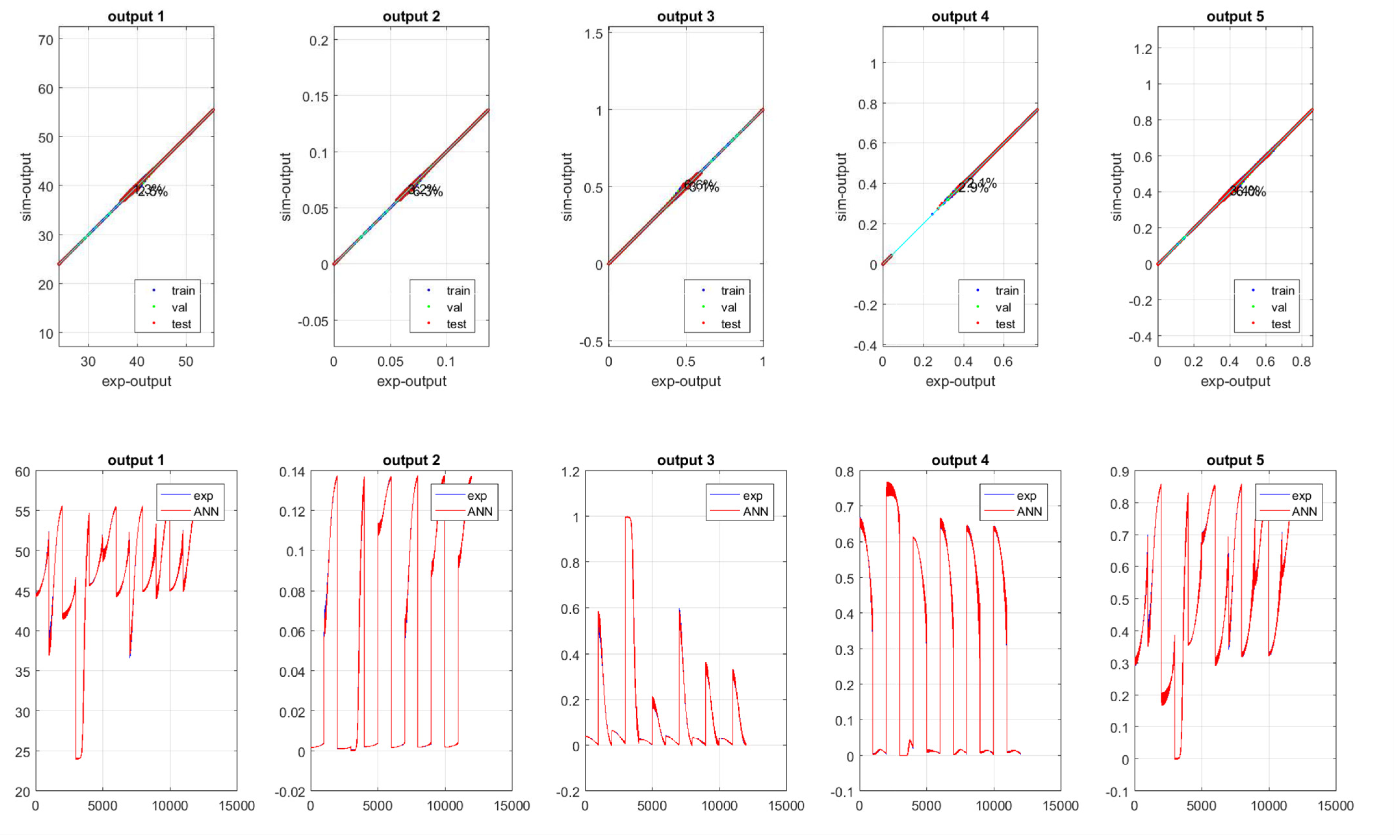
5.4. Results from ANN Modeling

Within the ANN modeling, 4410 different networks are varied by varying the number of neurons, the number of hidden layers, and the transfer function. The best network has been detected with two hidden layers with 16 neurons each (logsig 16, logsig16 and logsig 1). Levenberg–Marquardt backpropagation (trainlm) is used as the training algorithm. The maximum number of hidden layers has been limited to two and the number of neurons to 16 in order to limit the time required for training and validation. The results of the total output and the training, validation, and unseen data of the ANN are shown in Figure 22a through Figure 22b. Figure 22c shows the direct comparison of the respective hardness values of the experiments and the calculated hardness values of the ANN.

The regression lines show a good agreement between the experimental and ANN results. The regression value of the unseen data (see Figure 22b: test (red)) is R² = 0.947. Individual hardness values show larger deviations compared to the experimental values; see Figure 22b (98.2% deviation between simulated and experimental measured value). However, these deviations also indicate deviating experimental measurement data, measurement errors, or deviations in the material (e.g., segregation, etc.); see Figure 22d.

This measuring point has an experimentally determined hardness of approx. 15 HRC and leads to a deviation of 98.2% for the selected ANN in the test data (unseen). The ANN calculates a value of approximately 29.5 HRC for this point. This value generated by the ANN fits better into the results. The following figures show the experimentally determined hardness values in comparison with the calculated hardness of the ANN for selected examples with different geometries; see Figure 23a. The hardness within the selected experimental space can be mapped by the ANN.

The results of the calculations from the non-experimental parameter variations within the experimental space are shown in Figure 23b for a pressure of 8 bar. Such calculations outside the experimental space are also feasible; likewise, the most extrapolations should only be considered with great reservation, since larger deviations may occur. An extension of the ANN to other heat treatment parameters seems conceivable here.

Another ANN has been created and trained based on the FEM results, which takes into account the local HTC determined by the CFD simulation; compare Figure 21b. The results of the total output and the training, validation, and unseen data of the ANN are shown in Figure 23c and Figure 24. The outputs 1–5 are the hardness and volume fraction of microstructural constituents (Figure 15b). Also, 4410 different networks were varied while varying the number of neurons, the number of hidden layers, and the transfer function. The best network has been detected with two hidden layers with 16 neurons each (logsig 16 and purelin 5). Levenberg–Marquardt backpropagation (trainlm) is used as the training algorithm. The maximum number of hidden layers has been limited to two and the number of neurons to 16 in order to limit the time required for the training and validation. The regression lines show very good agreement between the FEM simulation and the ANN results. The regression value of the unseen data (see Figure 24: test (red)) is R² ≈ 1 for almost all the output variables.

This very good agreement is due to the fact that certain physical models are used for the numerical simulation, so that outliers, which can occur within the experimental data, do not occur. The maximum deviation for the generated ANN is 6.6%. However, the FEM simulation can deviate from the real experiments and additionally the FEM simulation requires validation.

Furthermore, it is possible to optimize the gas pressure and thus the gas consumption in the heat treatment process by means of the ANN. The developed ANN is able to create forecasts of the hardness depending on the process parameters. This is illustrated by the example of varying gas pressure. The ANN is used to set up a virtual test chamber, i.e., the gas pressure is varied between 6 bar and 12 bar in 0.1 bar steps. The user specifies a minimum hardness and it is checked regarding at which minimum gas pressure the required (targeted) minimum hardness is present in the component.

The ANN allows the calculation of hardness values as a function of pressure for different geometries and positions, so that it is possible to identify at which gas pressure the required minimum hardness is achieved. Figure 25b shows the calculated mean values as well as minimum and maximum values for the disc at position T-1-1 (top surface) of 42CrMo4. This optimization is possible not only for the individual geometries, but also for the complete batches.

The potential gas savings are approximated by the equation Equation (10) used for the gas consumption.

$$V_{\mathit{Gas}}\left(m^3\right)=V_{\mathit{Chamber}}\left(m^3\right)·p_{\mathit{Gas}}\left(\mathit{bar}\right)$$

(10)

At a gas pressure of 8 bar, a slightly different behavior of the sample is noticeable (Figure 25a), since the symmetry of the hardness deviates compared to the other samples. A deviating behavior is also noticeable in Figure 25b between 7 and 9 bar. This highlights a weakness of the ANN and indicates that validation tests are required to validate the results of the ANN. The gas pressure of 8 bar has not been included in the experiment plan. However, only two pressure variations (6 bar and 10 bar) have been tested experimentally. Thus, more grid points of the pressure (simulative or experimental) should be provided for training the grid. In future work, the optimization can also be extended with respect to the energy consumption of the motor of the ventilator, so that the optimal settings with respect to the gas and energy consumption can be attained. This demands the results with the variation of the ventilator speed either experimentally or simulative, for instance, by means of the CFD simulations.

The parameter variation of the gas pressure and ventilator speed cannot be directly transferred to other heat treatment furnace systems. This is due to the deviating chamber dimensions, different flow profile, flow velocity and/or also variations with the heating behavior. Different furnace systems even with identical process parameters can exhibit quantitatively deviating hardness results, even when qualitatively similar results are observed. One similar example is presented in Figure 26a,b. Another industrial heat treatment chamber larger than the Ipsen chamber (considered in this study) is used. This also confirms that somewhat similar cooling trends (qualitatively) are observed even if the chamber dimensions are deviating. This behavior implies that the cooling curves may be similar but with a shift in the temporal scale. For the application of the ANN, the ANN must be adapted for the particular furnace system or system type. Parameters that take these influences into account can be, for example, the respective chamber volume, the flow velocity, or the HTC. Further tests can be carried out with different quenching plants in order to accordingly extend the training data of the ANN to include the influence of different quenching plants (chamber dimension). In principle, this work has shown that the flow behavior and the local HTC can be represented by the CFD simulations and can be used for training the ANN. If corresponding CFD models are available for the different furnaces or chamber dimensions, it is possible to train the ANN for different chamber sizes.

6. Conclusions

The heterogeneous gas quenching process in the heat treatment of steel specimens has been analyzed based on the experiments, numerical simulations, and artificial intelligence schemes, where the influence of probe geometry, probe materials, flow velocity, gas pressure and batch configuration has been investigated.

Single-probe wind tunnel experiments reveal the heat transfer coefficient (HTC) as a function of local position, sample geometry, and flow velocity. The probe edge (side) possesses higher HTC as the flow velocity accelerates towards the probe edge. Experiments in a model quenching chamber (cold experiments) analyzing the flow field illustrate that the batch configuration and probe geometry significantly influencethe surrounding flow field and the flow below the top layer. A flow acceleration (nozzle effect) occurs through the probe holes and the gap area between the probes within the batch, which leads to increasing the quenching intensity of subsequent layers within the batch compared to the top layer. The disc batch generates higher flow velocity than the ring batch. The flow field for the ring batch does not have higher velocity peaks such as in the disc batch, resulting in a more uniform cooling process.

The experiments within an industrial heat treatment gas quenching process (Ipsen plant) reveal the significant areas of the quenching trend for batch quenching. The quenching intensity is a function of the probe location within the batch. Due to the flow acceleration through the gaps between the probes, the probes from the bottom layer cool down faster than the top layer. It is observed that the outer probes are generally faster than the inner probes. The flow velocity, gas pressure, probe geometry, probe material and batch configuration influence the quenching process. Increased flow velocity and the gas pressure improves the quenching intensity. The staggered configuration provides improved cooling rates compared to the inline configuration. The quenching intensity increases with lower probe mass and a batch with lower mass such as the rings possessing a uniform cooling trend within the batch.

The observed hardness values correlate with the observed temperature measurements and HTC investigations. A lower local HTC corresponds to a lower local cooling rate and local hardness. An increased probe volume or probe mass results in a lower cooling rate.

Numerical CFD models are developed and validated with experiments. The numerical simulations show that the HTC can be controlled with the flow velocity and the gas pressure. As observed in the experiments, the probe edges exhibit higher HTC from the accelerated flow towards the probe edge. However, a symmetric HTC distribution is observed for the single-probe quenching. In the case of a batch simulation with flow from the top to bottom, the bottom layer has improved HTC due to the flow acceleration through gaps or probe holes of the top layer. It is observed from the batch simulation that the HTC distribution with the batch is not symmetric as in the single-probe simulation. Improved HTC values are generally obtained with the staggered configuration. The HTC increases with the flow velocity and the gas pressure. From the simulation results, a correlation for the maximum and average HTC for the disc batch (42CrMo4) has been developed, which is able to predict the HTC for different flow velocity and gas pressure ranges.

Microstructural transformations and hardness in heterogeneous gas quenching can be depicted using FEM simulations. It is observed that JMATPro is a suitable tool for calculating the structure-dependent material parameters, which can be used for the FEM simulations. The transformation data in particular have a major influence on the simulation results of the microstructure and hardness development in heterogeneous gas quenching and should therefore be verified with experiments. The coupling of the CFD simulation data with the boundary conditions for the FEM led to a very consistent cooling process analysis. By varying the process parameters, it is possible to create a virtual test room and generate a variety of virtual measurement data (keyword: digital twin).

Various ANNs have been developed based on the experimental results as well as on the CFD and the FEM simulation results. By expanding the training database and using the CFD, FEM and ANN, the previous design can be improved compared to “trial and error” and/or table books. The possibilities of process optimization using the example of gas consumption have been presented. In future work, it is conceivable to implement a monitoring tool that directly indicates deviating process parameters/influencing variables during the heat treatment process and the effects on the heat treatment result. The developed ANN framework based on the experiments as well as the CFD/FEM simulations can be extended further to be used as a prediction tool for the heterogeneous gas quenching process.

This paper illustrates the ANN-derived prediction results for the high-pressure gas quenching process parameters, thereby enabling the heat treatment industries to achieve further process optimization in terms of energy consumption and resource utilization.

Future studies should consider the effect of variations in gas type, sample material and geometry to extend the applicability of the derived model. The introduction of physics-informed neural networks (PINNs) appears to be a promising tool for future investigations.

References

1. Schmidt, R.R. Zur Thermo-Fluid-Dynamik beim Hochdruckgasabschrecken: Experimentelle und Numerische Analyse der Hochdruckgasabschreckung Metallischer Bauteile zur Steigerung von Prozesshomogenität und-Intensität. Ph.D. Thesis, Fachbereich Produktionstechnik, Universität Bremen, Bremen, Germany, 2013. [Google Scholar]
2. Bucquet, T.; Fritsching, U. Evaluating Heat Transfer Conditions in Gas Cooling for Complex Specimen Geometries. HTM J. Heat Treat. Mater. 2014, 69, 148–154. [Google Scholar] [CrossRef]
3. Stephan, P.; Kabelac, S.; Kind, M.; Mewes, D.; Schaber, K.; Wetzel, T. VDI-Wärmeatlas (Fachlicher Träger VDI-Gesellschaft Verfahrenstechnik und Chemieingenieurwesen); Springer: Berlin/Heidelberg, Germany, 2018. [Google Scholar]
4. Jung, M.; Lee, S.-J.; Lee, W.-B.; Moon, K.I. Finite Element Simulation and Optimization of Gas-Quenching Process for Tool Steels. J. Mater. Eng. Perform. 2018, 27, 4355–4363. [Google Scholar] [CrossRef]
5. Bucquet, T. Flow Conditioning in Heat Treatment by Gas and Spray Quenching. Ph.D. Thesis, Produktionstechnik, Universität Bremen, Bremen, Germany, 2017. [Google Scholar]
6. Narayan, N.M.; Moqadam, S.I.; Ellendt, N.; Fritsching, U. Multiphase numerical modeling and investigation of heat transfer for quenching of spherical particles in liquid pool. Int. J. Therm. Sci. 2023, 186, 108016. [Google Scholar] [CrossRef]
7. Narayan, N.M.; Gopalkrishna, S.B.; Mehdi, B.; Ryll, S.; Specht, E.; Fritsching, U. Multiphase numerical modeling of boiling flow and heat transfer for liquid jet quenching of a moving metal plate. Int. J. Therm. Sci. 2023, 194, 108587. [Google Scholar] [CrossRef]
8. Ferrari, J.; Lior, N.; Slycke, J. An evaluation of gas quenching of steel rings by multiple-jet impingement. J. Mater. Process. Technol. 2003, 136, 190–201. [Google Scholar] [CrossRef]
9. Lior, N. The cooling process in gas quenching. J. Mater. Process. Technol. 2004, 155–156, 1881–1888. [Google Scholar] [CrossRef]
10. Elkatatny, I.; Blicblau, A.S.; Das, S.; Doyle, E.D. Numerical analysis and experimental validation of high pressure gas quenching. Int. J. Therm. Sci. 2003, 42, 417–423. [Google Scholar] [CrossRef]
11. Lior, N.; Papadopoulos, D. Gas-Cooling of Multiple Short Inline Disks in Flow along Their Axis. J. ASTM Int. 2008, 6, JAI101849. [Google Scholar] [CrossRef]
12. Wang, J.; Gu, J.; Shan, X.; Hao, X.; Chen, N.; Zhang, W. Numerical simulation of high pressure gas quenching of H13 steel. J. Mater. Process. Technol. 2008, 202, 188–194. [Google Scholar] [CrossRef]
13. Sugimoto, T.; Qin, M.; Watanabe, Y. Computational Study of Gas Quenching on Carburizing Hypoid Ring Gear. BHM Berg Hüttenmännische Monatshefte 2006, 151, 456–461. [Google Scholar] [CrossRef]
14. Narayan, N.M.; Landgraf, P.; Lampke, T.; Fritsching, U. Experimental and numerical investigation of heterogenous gas quenching for determining optimal heat treatment parameters. In Proceedings of the 27th IFHTSE Congress and European Conference on Heat Treatment, Salzburg, Austria, 5–8 September 2022; pp. 81–87. [Google Scholar]
15. Landgraf, P.M.; Narayan, N.M.; Fritsching, U.; Lampke, T. Development of a prognosis tool to predict heat treatment results for heterogeneous gas quenching of steels. In Proceedings of the 31st International Conference on Metallurgy and Materials, Brno, Czech Republic, 18–19 May 2022; pp. 395–401. [Google Scholar] [CrossRef]
16. Wróbel, J.; Kulawik, A.; Bokota, A. Artificial Neural Network to the Control of the Parameters of the Heat Treatment Process of Casting. Arch. Foundry Eng. 2015, 15, 119–124. [Google Scholar] [CrossRef]
17. Wróbel, J.; Kulawik, A. Calculations of the heat source parameters on the basis of temperature fields with the use of ANN. Neural Comput. Appl. 2018, 31, 7583–7593. [Google Scholar] [CrossRef]
18. Muñoz-Rodenas, J.; García-Sevilla, F.; Coello-Sobrino, J.; Martínez-Martínez, A.; Miguel-Eguía, V. Effectiveness of Machine-Learning and Deep-Learning Strategies for the Classification of Heat Treatments Applied to Low-Carbon Steels Based on Microstructural Analysis. Appl. Sci. 2023, 13, 3479. [Google Scholar] [CrossRef]
19. Chong, Z.S.; Wilcox, S.; Ward, J. The Use of Artificial Intelligence in the Modelling and Heat Treatment Parameters Identification for Alloy-Steel Re-Heating Process. In Proceedings of the Volume 1: 20th Biennial Conference on Mechanical Vibration and Noise, Parts A, B, and C, Long Beach, CA, USA, 24–28 September 2005. [Google Scholar]
20. Opel, L. Kalibration einer Oberflächensonde; Studienarbeit; Universität Bremen: Bremen, Germany, 2008. [Google Scholar]
21. Glue-on Filmprobe. Available online: https://www.dantecdynamics.com/components/hot-wire-and-hot-film-probes/miscellaneous-probes/ (accessed on 20 November 2023).
22. XY Positioning Stage. Available online: https://www.optosigma.com/ (accessed on 20 November 2023).
23. Datalogger. Available online: https://www.flukeprocessinstruments.com/ (accessed on 20 November 2023).
24. Tell, J. Entwicklung eines Strömungs-Messystemes zur Qualifizierung von Gas Abschreckprozessen. Diploma Thesis, Productionstechnik, Universität Bremen, Bremen, Germany, 2012. [Google Scholar]
25. ANSYS. ANSYS ICEM CFD User Manual; ANSYS: Canonsburg, PA, USA, 2012. [Google Scholar]
26. ANSYS. ANSYS Fluent User’s Guide; ANSYS: Canonsburg, PA, USA, 2018. [Google Scholar]
27. Kempf, A. Lecture Manuscript for Turbulence; University of Duisburg-Essen: Essen, Germany, 2015. [Google Scholar]
28. Baehr, H.D.; Stephan, K. Wärme- und Stoffübertragung; Springer: Berlin/Heidelberg, Germany, 2013. [Google Scholar]
29. Schulze, P.; Schmidl, E.; Halle, T.; Lampke, T. Simulation der Wärmebehandlung von Stahl unter Berücksichtigung der Gefügeentwicklung. In Proceedings of the Energy-Efficient Technologies in Production ICMC 2014, Chemitz, Germany, 7–11 July 2014. [Google Scholar]
30. DEFORM-3D v10.2, User’s manual, Columbus, Ohio. Available online: https://www.deform.com (accessed on 20 November 2023).
31. JMatPro. Available online: https://www.sentesoftware.co.uk/site-media (accessed on 17 March 2024).
32. Diemar, A. Simulation des Einsatzhärtens und Abschätzung der Dauerfestigkeit einsatzgehärteter Bauteile. Ph.D. Thesis, Bauhaus-Universität, Weimar, Germany, 2007. [Google Scholar]
33. Macchion, O.; Zahrai, S.; Bouwman, J.W. Heat transfer from typical loads within gas quenching furnace. J. Mater. Process. Technol. 2006, 172, 356–362. [Google Scholar] [CrossRef]
Figure 1. Sample geometries for investigation such as disc, disc with hole, and ring; plastic probes for cold experiments.
Dynamics 04 00023 g001
Figure 2. Experimental setup. (a) Suction wind tunnel for measuring HTC. (b) Model gas quenching chamber for investigating flow field with batches (cold experiments). (c) Two-chamber heat treatment plant (Ipsen) for quenching of batches.
Dynamics 04 00023 g002
Figure 3. (a) A two-layered inline batch from disc probes with measurement systems below the second layer for quenching in the Ipsen plant. (b) The probe designation considered in this work within the batch for Ipsen plant experiments. (c) The CAD diagram showing measurement locations within the probe volume for thermocouples; the thermocouple directed from the bottom to top surface. (d) The thermocouple supported by an additional support plate at the bottom surface of the probe to be quenched.
Dynamics 04 00023 g003
Figure 4. (a) The 1D-CTA probe for velocity measurement. (b) The pitot tube for velocity measurement. (c) The film probe (glue-on) from DANTEC [21] for determining the HTC. (d) XY positioning stages with the flow measuring probe [22] assembled inside the model chamber for analyzing the flow behavior past batches.
Dynamics 04 00023 g004
Figure 5. The pattern of the hardness measurements (indentations) for different probe geometries such as a disc, disc with a hole, and ring at the top and bottom probe surfaces.
Dynamics 04 00023 g005
Figure 6. (a) Flow velocity at wind tunnel center measured with pitot tube and 1D-CTA probe. (b) Measurement repeatability with wind tunnel for HTC at mean flow of 7.8 m/s (16 Hz).
Dynamics 04 00023 g006
Figure 7. HTC measurements for the disc probe at two local positions and for varying mean flow velocity (7.8, 9.8, and 12 m/s).
Dynamics 04 00023 g007
Figure 8. The flow field analysis within the model chamber. (a) The support frame for holding samples and the flow measurement system below the support frame with the xy positioning stage. (b) Sample two-layered inline discs with hole arrangement inside the model chamber. (c) The flow measurement window of 200 × 300 mm2.
Dynamics 04 00023 g008
Figure 9. (a) Flow field measurement for an empty model chamber at a distance of 130 mm (inlet position) above the top layer with varying flow rates resp. to motor frequency. (b) Flow field measurement at a distance of 20 mm below the bottom layer for inline two-layered batches with discs, discs with a hole and rings at a motor frequency of 30 Hz resp. to a volumetric flow rate of 3.48 m3/s.
Dynamics 04 00023 g009
Figure 10. (a) Measurement reproducibility for 10 bar N2 quenching measured at the austenitic probe (1.4301/disc) with Tf = 850 °C and tf = 75 min. (b) The quenching trend within an inline disc batch during 10 bar N2 quenching with Tf = 850 °C and tf = 75 min. (c) Quenching intensity during 10 bar N2 quenching within a disc probe (42CrMo4) with Tf = 850 °C and tf = 75 min at probe position T-2-2. (d) Quenching intensity during 10 bar N2 quenching within a ring probe (42CrMo4) with Tf = 850 °C and tf = 75 min at probe position T-2-2.
Dynamics 04 00023 g010
Figure 11. (a) Influence of gas pressure on sample cooling within inline disc batch configuration (42CrMo4); N2 quenching with Tf = 850 °C and tf = 75 min. (b) Influence of specimen geometry on t800/500 for inline batch (42CrMo4) during 10 bar N2 quenching with Tf = 850 °C and tf = 75 min. (c) Influence of specimen material on quenching for inline disc batch (42CrMo4) during N2 quenching with Tf = 850 °C and tf = 75 min.
Dynamics 04 00023 g011
Figure 12. HRC–hardness of heat-treated specimen at top and bottom surfaces. (a) Disc at position T-1-1 (42CrMo4—10 bar). (b) Disc at position T-1-1 (42CrMo4—6 bar). (c) Ring at position T-1-1 (42CrMo4—10 bar). (d) Ring at position T-2-3 (100Cr6—10 bar).
Dynamics 04 00023 g012
Figure 13. Computational domain and spatial discretization for (a) single-probe CFD simulation; (b) disc batch CFD simulation.
Dynamics 04 00023 g013
Figure 14. (a) Complex interactions in heat treatment simulation using FEM, taking into account microstructural transformation, adapted from [29,30]. (b,c) Example of selected material data for 42CrMo4 from JMatPro®: thermal conductivity and volumetric heat capacity.
Dynamics 04 00023 g014
Figure 15. (a) An example of the structure, input, and output parameters of the ANN, which has been created and trained based on the experimentally determined hardness values. (b) An example of the structure, input and output parameters of the ANN created and trained on the basis of the hardness values determined by CFD and FEM simulations.
Dynamics 04 00023 g015
Figure 16. (a) Validation of numerical model with experiment, HTC for disc probe with Vavg = 7.8 m/s and Tprobe = 100 °C, and corresponding HTC contours [14]. (b) Velocity vector for simulation with Vavg = 7.8 m/s and Tprobe = 100 °C for disc probe [14]. (c) Influence of flow velocity on HTC with Tprobe = 100 °C for disc probe.
Dynamics 04 00023 g016
Figure 17. Simulation results for the ring with Vavg = 7.8 m/s and Tprobe = 100 °C. (a) The velocity vector; (b) HTC contours.
Dynamics 04 00023 g017
Figure 18. (a) HTC contours and velocity vectors during N2 quenching with Tprobe = 850 °C (42CrMo4), P = 10 bar and Vavg = 13.4 m/s. (a) Inline disc batch. (b) Inline ring batch. (c) Staggered disc batch.
Dynamics 04 00023 g018
Figure 19. Influence of (a) gas pressure and (b) flow velocity during inline batch N2 quenching with Tprobe = 850 °C (42CrMo4).
Dynamics 04 00023 g019
Figure 20. Impact of flow velocity and gas pressure on (a) HTCmax and (b) HTCavg based on correlations developed for disc batch (T-2-2/T-2-3) for 42CrMo4 with Tprobe = 850 °C during N2 quenching.
Dynamics 04 00023 g020
Figure 21. (a) Comparison of simulated hardness values based on different transformation data with experimentally determined hardness values. (b) Examples of selected FEM results (2D and 3D representation) for Tprobe = 850 °C and P = 10 bar. (c) Comparison of experimentally (Exp) determined cooling curve from sample core with simulated (Sim) cooling curve (FEM) based on the CFD boundary conditions (HTC) for disc, disc with hole, and ring specimen geometries during 10-bar quenching from Tf = 850 °C.
Dynamics 04 00023 g021
Figure 22. (a) Regression total output ANN with target variable. (b) Differentiation between training, validation and test data. (c) Hardness values of experiment and ANN. (d) Deviating measured values marked by red arrow.
Dynamics 04 00023 g022
Figure 23. (a) Hardness determined experimentally and from ANN for probes’ disc, disc with hole, and ring. (b) Example of calculated hardness distribution in HRC for disc at position T-1-1 (42CrMo4) at gas quenching pressure of 8 bar. (c) Regression total output ANN with target value based on ANN/FEM results.
Dynamics 04 00023 g023
Figure 24. (Top) Differentiation between training, validation, and test data for outputs; (Bottom) output values of the experiment and ANN; outputs 1–5 are the hardness and volume fraction for austenite, pearlite, bainite and martensite.
Dynamics 04 00023 g024
Figure 25. (a) The variation of the gas pressure on the example disc T-1-1 (top surface) from 42CrMo4; the 8-bar deviate forms the resulting image. (b) The variation of the mean values calculated by the ANN as well as the maxima and minima and optimum at the required minimum hardness (for example, 40 HRC requires quenching with min. of 10.25-bar gas pressure); the deviation at 8 bar is also observed here.
Dynamics 04 00023 g025
Figure 26. Comparison of hardness profiles from (a) Ipsen batch heat treatment experiment for disc batch and (b) other industrial chambers for disc batch with 10 bar N2 quenching; global scale (global maximum hardness for hardness legend) and local scale (local maximum hardness for hardness legend) illustrated for qualitative comparison.
Dynamics 04 00023 g026