Abstract
This study investigates mixed convection flow over a vertical thin needle with variable surface heat, mass, and microbial flux, incorporating the influence of gyrotactic microorganisms. The governing partial differential equations are transformed into ordinary differential equations using appropriate similarity transformations and then solved numerically by employing MATLAB’s Bvp4c solver. The primary focus lies in examining the influence of various dimensionless parameters, including the mixed convection parameter, power-law index, buoyancy parameters, bioconvection parameters, and needle size parameters, on the velocity, temperature, concentration, and microbe profiles. The results indicate that these parameters significantly affect the surface (wall) temperature, fluid concentration, and motile microbe concentration, as well as the corresponding velocity, temperature, concentration, and microorganism profiles. The findings provide insights into the intricate dynamics of mixed convection flow with bioconvection and have potential applications in diverse fields such as biomedicine and engineering.
1. Introduction
Researchers have devoted increasing attention to studying mixed convection in recent years due to its significant role in numerous technological and industrial applications. Mixed convection, which combines both forced and free convection, occurs when fluid flow is influenced by both external mechanical forces (such as pumps or fans) and buoyancy forces arising from temperature differences within the fluid. This phenomenon is crucial in many systems where heat transfer efficiency plays a key role in operational performance. Examples include heat exchangers operating in low-velocity environments, solar collectors exposed to wind currents, and emergency cooling systems for nuclear reactors. In these scenarios, controlling and optimizing the heat transfer process are essential for safety and efficiency. Mixed convection is often observed in environmental processes, such as atmospheric boundary layer flows, and industrial systems, like cooling technologies used in reactors and electronics. The growing interest in mixed convection is largely driven by its significance in numerous practical engineering applications, as demonstrated by various studies.
Nasir et al. [1] examined stagnation-point flow and heat transfer over a permeable quadratically stretching or shrinking sheet, emphasizing the importance of mixed convection in optimizing fluid flow and heat transfer around complex surfaces. This study is particularly relevant for manufacturing processes such as material extrusion and coating. Aly and Raizah [2] explored mixed convection in an inclined nanofluid-filled cavity saturated with a partially layered porous medium, shedding light on how mixed convection in porous structures can enhance thermal efficiency in systems like solar collectors and insulation technologies. Similarly, Rashid et al. [3] conducted a numerical investigation of magnetohydrodynamic hybrid nanofluid flow over a stretching surface, focusing on the impact of mixed convection and strong suction in improving heat transfer efficiency. Their study is crucial for advanced cooling systems and magnetic field control applications, such as electronics and magnetic resonance technologies. These studies collectively demonstrate the broad applicability of mixed convection in enhancing heat transfer and fluid flow performance across diverse engineering systems.
Numerous researchers, such as Raju et al. [4] and Ahmad et al. [5], have focused on studying mixed convection over various types of surfaces to understand the interaction between forced convection, driven by external forces, and natural convection, which is buoyancy-induced. The primary factor that governs this interaction is heat flux—the rate at which heat energy transfers across a surface. In mixed convection flows, managing heat flux is vital as it directly influences temperature distribution within the fluid and along solid boundaries. Heat flux dictates the overall efficiency of heat exchange in applications such as HVAC systems, geothermal energy extraction, and electronics cooling. The analysis of heat flux is particularly important in boundary layer studies, where the fluid’s temperature and velocity profiles change rapidly near solid surfaces. In these regions, the complex interplay between buoyancy and mechanical forces can lead to intricate heat transfer patterns that are challenging to predict. By understanding and controlling heat flux, engineers can develop more efficient thermal systems that optimize heat dissipation or retention, depending on the requirements of the specific application. Heat flux and mixed convection studies have shown their importance in various manufacturing processes, especially where uniform or non-uniform heat distribution affects product quality and efficiency. For instance, Ahmed et al. [6] recently investigated mixed convective Williamson fluid flow with variable thermal conductivity, providing insights into how changes in material properties affect heat transfer. Similarly, Everts et al. [7] examined forced convective flow through a horizontal tube with constant surface heat flux, offering valuable information for designing more efficient heat exchanger systems.
Beyond conventional heat transfer studies, bioconvection introduces additional complexity by involving self-propelled microorganisms that actively influence flow behaviour. Bioconvection in fluid dynamics refers to the phenomenon where self-propelled microorganisms, such as algae and bacteria, react with oxygen gradients (oxytaxis), rotation (gyrotaxis), or gravity. Motile bacteria swim upwards in the system due to their greater density compared to the surrounding liquid. This behaviour results in the development of diverse flow patterns, as extensively documented in studies conducted by Khan et al. [8], Saleem et al. [9], Mahdy et al. [10], and others. Researchers have also investigated nanofluid bioconvective flow around various geometric configurations. Gyrotactic bacteria play a crucial role in bioconvection by coordinating group movements that substantially impact ecological dynamics. Their navigational proficiency in locating nutrient-abundant areas plays a role in the transportation of nutrients, affecting the spatial arrangement of microorganisms in aquatic habitats. The bioconvection patterns that are created also contribute to the biological pump by enabling the upward movement of organic materials and nutrients. Moreover, the ability of gyrotactic microorganisms to respond to light gradients improves their capacity to perceive and understand their surroundings. In addition to ecological ramifications, examining these microorganisms offers a significant understanding of thermo-bioconvection, microbial augmentation, bio-microsystems, biofuels, and other bioengineering systems.
Several studies have explored the impact of gyrotactic microorganisms on mixed convective nanofluid flows across various geometries. Sudhagar et al. [11] investigated how gyrotactic microorganisms influence mixed convective nanofluid flow past a vertical cylinder, emphasizing their role in modifying heat transfer characteristics. Mallikarjuna et al. [12] extended this study by studying mixed bioconvection flow around a vertical slender cylinder, highlighting the intricate dynamics introduced by gyrotactic microorganisms in nanofluids. Rashad and Nabwey [13] further analyzed the gyrotactic mixed bioconvection flow of nanofluids around a circular cylinder with convective boundary conditions, providing insights into boundary layer behaviour. Mahdy [14] examined the unsteady mixed bioconvection of Eyring–Powell nanofluid containing motile gyrotactic microorganisms near a stretching surface, contributing to understanding complex flow behaviour in bioconvective systems.
Similarly, Waqas et al. [15] investigated magneto-Burgers nanofluid flow with motile microorganisms near a stretching cylinder or plate, focusing on stratified flows and variable thermal conductivity. Most recently, Bilal et al. [16] conducted a comparative study on the heat transfer characteristics of Carreau nanofluids containing gyrotactic microorganisms, providing new insights into the role of fluid rheology and microorganism behaviour in optimizing thermal systems. Alharbi et al. [17] investigated the importance of gyrotactic microorganisms in a tangent hyperbolic nanofluid flowing across a thin surface. Alam et al. [18] studied gyrotactic microbial flow under thermal radiative conditions over a dual-stretched surface. In recent studies, Khan et al. [19] and Yasmin [20] investigated hydromagnetic bioconvection flow with nanofluid over stretching surfaces. The effect of Stefan blowing and gyrotactic bacteria on bio-nano convective flow past a needle is reported by Beg et al. [21]. These studies collectively demonstrate the significance of incorporating gyrotactic microorganisms in enhancing nanofluid heat transfer performance in various industrial applications.
Building on the role of gyrotactic microorganisms in fluid dynamics, researchers have also focused on the unique flow characteristics surrounding a thin needle, which has significant applications in biomedical and engineering fields, including cancer treatment and transdermal medicine delivery. Experimental research on momentum and heat transfer by analyzing slender needle flow is essential. This phenomenon arises due to the movement of the needle, which causes disturbances in the flow of the free stream. Thus, this topic is vital for hot anemometers used to measure wind velocity, transportation systems, geothermal power generation, fibre technology, lubrication, aerospace, wire coating, metal spinning, micro/nanoscale equipment, and underground nuclear waste disposal. Thin needles have paraboloids of revolution geometry and are thinner than boundary layer thickness. Grosan and Pop [22] were the first to study nanoparticles’ effect on thin needle flow. Soid et al. [23] applied this to a needle in a nanofluid. Hayat et al. [24] studied nano-liquid flow where a thin needle near a stagnation point changed surface heat flux. Ali et al. [25] studied mixed convective nanofluid flow over a needle. Salleh et al. [26] examined how a heat source and a chemical reaction affect nanofluid flow around a thin needle in a stability analysis. Waini et al. [27] studied hybrid nanofluid flow through a thin needle.
So far, research on free or mixed convection boundary layer flow over vertical thin needles has primarily focused on stationary needles in a viscous, incompressible fluid. Previous studies have largely examined heat and mass transfer under isothermal or non-isothermal conditions, considering constant and variable wall heat flux. However, the analysis presented here addresses a critical gap in the recent literature by analyzing the influence of gyrotactic microorganisms on mixed convection flow over a thin needle under variable surface heat, mass, and microbial flux conditions. This framework is distinct due to its integration of bioconvection dynamics, particularly the complex interactions between mixed convection and microbial motility, using the Darcy model and introducing new similarity transformations and dimensionless quantities. The present study assists the existing literature in responding to the following questions:
- How do variable surface fluxes influence the heat and mass transfer characteristics in mixed bioconvection flow around vertical thin needles?
- How do the values of the mixed convection parameter influence flow profiles and describe the transition from forced convection to mixed convection behaviour with variations in velocity, temperature, concentration, and microorganism distribution?
- How can the motility rate, heat and mass transfer rates, and flow rate be influenced by different emerging parameters such as mixed convection and buoyancy parameters?
- How do different bioconvection parameters, such as Peclet and Bioconvection Lewis numbers, influence the overall efficiency of heat and mass transfer?
- How do variations in needle size affect the flow dynamics and heat transfer characteristics in mixed bioconvection around vertical thin needles?
- How do transient effects impact the flow behaviour and heat transfer characteristics when transitioning from isothermal to non-isothermal conditions?
In addressing the research question of how mixed convection parameters influence flow profiles and the transition from forced convection to mixed convection behaviour, this study aims to utilize the Darcy model to explore the behaviour of gyrotactic microorganisms around thin needles. This analysis encompasses various needle sizes and both isothermal and non-isothermal conditions. It also examines how different bioconvection parameters impact the flow profile and transition dynamics. The Darcy model is advantageous for fluid flow analysis as it simplifies the complex interactions of microorganisms and fluid dynamics, making it easier to implement and interpret than more complicated models. Additionally, this study introduces new dimensionless quantities and similarity transformations for simulation, enhancing its novelty and uniqueness. Including variable surface heat flux in the boundary conditions is crucial, as it directly impacts heat transfer efficiency and affects the behaviour of motile microorganisms around the needle. By examining these interactions with the Darcy model, the study aims to provide valuable insights into heat, mass, and motile microbe flux dynamics over thin needles. The findings have potential applications across various industries, including food and pharmaceuticals, chemical processing equipment, fuel cell technology, and enhanced oil recovery.
The remainder of this manuscript is structured as follows: Section 2 details the mathematical model and governing equations for the mixed convection flow around a thin needle, while Section 3 describes the numerical methods used to solve these equations. Section 4 presents the results and an in-depth discussion of the findings, and finally, Section 5 provides conclusions and suggests potential avenues for future research.
2. Model Formulation
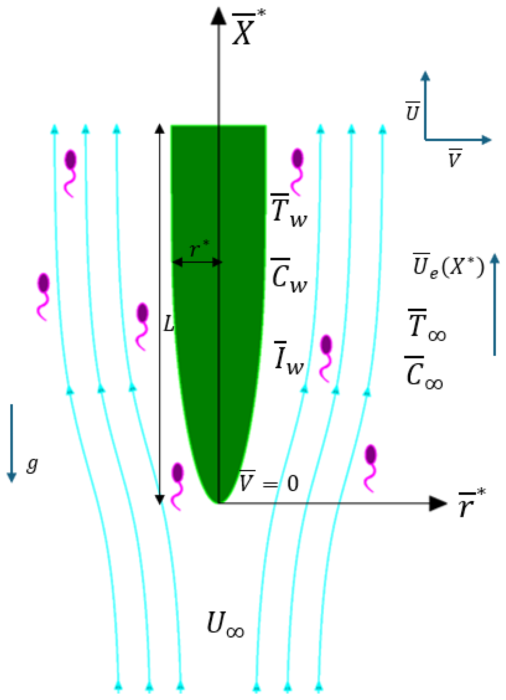
Following the Introduction Section, this section outlines the mathematical model governing the mixed convection flow around a vertical thin needle with gyrotactic microorganisms. This study examines the 2-D laminar flow of a fluid surrounding a vertical thin needle. A needle is deemed thin when its thickness is not greater than the boundary layer that forms over it. The flow is influenced by variations in heat, mass, and the movement of microorganisms. Additionally, the presence of gyrotactic bacteria is taken into account. Figure 1 provides a visual representation of the computational domain and the system’s configuration. A vertical, thin needle defined by a radius is displayed alongside the flow model with system coordinates; where the − axis is measured from the leading edge of the needle, and the axial and radial coordinates and correspond to and , respectively. Variable mainstream velocity is considered to be subject to the variable heat flux , mass flux , and motile microbial flux .

Figure 1.
Flow diagram and graphical system.
In the Darcy model, the fluid flow through porous media is described focusing on the relationship between pressure gradients and fluid velocity. In the context of mixed convection flows around vertical thin needles, it simplifies analysis by assuming that flow is primarily governed by viscous forces rather than inertial effects. The model establishes a linear relationship between flow velocity and pressure gradient, allowing for the incorporation of buoyancy forces , which are significant in systems involving gyrotactic microorganisms. The Boussinesq approximation facilitates the analysis of buoyancy-driven flows by postulating that density variations are negligible except for their influence on the buoyancy force, which is considered variable otherwise. This assumption enables a more accurate formulation of the governing equations, rendering it particularly advantageous in the context of mixed convection flows around vertical thin needles. Under these assumptions along with the physical phenomena and Boussinesq approximations, the governing dimensional equations in cylindrical coordinates are as follows:
The corresponding boundary conditions are as follows:
Here, are the dimensional temperature, concentration, and volume fraction of motile microorganisms, respectively. is the permeability of the porous medium, is the fluid viscosity, is the density of the fluid, g is the acceleration due to gravity, is the thermal expansion coefficient, is the effective thermal diffusivity of the porous medium, is the thermal conductivity of the fluid, is the solute diffusivity, and is the diffusivity of the microorganism.
The formulation of the microorganism equation above integrates fluid dynamics with microbial behaviour, using parameters such as the chemotaxis constant, , and microbial cell speed, , to describe how microorganisms move and proliferate in response to their environment. The cell swimming speed indicates how quickly microorganisms can navigate through the fluid, impacting their ability to respond to environmental changes. Meanwhile, the microorganism diffusivity, , accounts for the random movement of microorganisms, which is essential for modelling their dispersion in the fluid.
The dimensional governing Equations (1)–(5), subject to boundary conditions (6) and (7), are nondimensionalized by following Beg et al. [21] and by incorporating characteristic length scale and velocity scale as listed below:
For a vertical thin needle, L is the length of the needle, and is the reference free-stream velocity.
The stream function, ψ, is defined as follows:
Using (8, 9), the resulting transformed equations are as follows:
The boundary conditions are as follows:
To better aid in interpreting the dimensionless parameters governing mixed bioconvection around a thin vertical needle, Table 1 summarizes the key dimensionless Pi-groups and their physical significance within the context of this study.

Table 1.
Defining dimensionless parameters.
Similarity transformations are now as follows:
Setting , the relationship explains the body’s shape and size with its surface assumed by , where is a cylinder, is a paraboloid (blunt-nosed shape), and is a cone.
Next, the transformations of ordinary differential equations are as follows:
The modified boundary conditions are as follows:
The definitions of surface temperature , surface fluid concentration and surface motile microorganism concentration are as follows:
Finally, using nondimensional and similarity transformations,
3. Numerical Method
To solve the governing equations developed in Section 2, this section presents the numerical approach adopted for analyzing mixed bioconvection around a vertical thin needle, utilizing MATLAB’s bvp4c solver and Maple’s dsolve algorithm.
In solving boundary value problems (BVPs) using MATLAB’s bvp4c function, the first step involves defining the system of ordinary differential equations (ODEs) representing the problem. Equation (7)–(10) can be rearranged as follows:
The MATLAB bvp4c function works based on the following workflow for solving boundary value problems for ordinary differential equations (ODEs):
- Function Structure: The syntax for bvp4c is sol = bvp4c(odefun, bcfun, solinit).
- ○
- odefun: A function that defines the system of ordinary differential equations. It should accept the independent variable (typically denoted as ) and a vector of dependent variables (denoted as ) and return the derivatives of .
- ○
- bcfun: A function that specifies the boundary conditions. It returns the residuals for the boundary conditions, ensuring they are satisfied at the endpoints of the interval.
- ○
- solinit: An initial guess for the solution structure, which is crucial for the convergence of the numerical method.
- Initial Solution Guess: solinit is an essential aspect of using bvp4c. Providing a good initial guess helps the solver converge to the correct solution.
- Transforming to First-Order Equations: Since bvp4c requires the governing equations to be expressed as a system of first-order ODEs, any higher-order equations must be rewritten accordingly. For this, let and
Then, the differential equations of the first-order are as follows:
The boundary conditions are defined by as the left boundary and as the right boundary.
- 4.
- Mesh Selection and Error Control: bvp4c automatically generates a mesh (grid of points) to evaluate the solution. It adapts the mesh based on the behaviour of the solution, refining it in regions where rapid changes occur. Error control is managed by analyzing the residuals of the continuous solution, allowing the solver to adjust the mesh and ensure that the solution is within a specified tolerance.
- 5.
- Output Structure: The output sol is a structure containing the solution information, including the mesh points and the corresponding values of the dependent variables. The solution can be evaluated at any point in the interval using the deval function, which interpolates the solution.
To validate the findings, the differential equations are once again solved numerically using Maple’s algorithm. Here is a detailed explanation of how the Maple algorithm operates in this context:
- Symbolic vs. Numerical Solutions: The dsolve command in Maple can provide both symbolic and numerical solutions. In the case of symbolic solutions, Maple attempts to find an exact expression for the solution of the differential equations.
- Defining the Problem: To use dsolve, users must first define the differential equations along with any initial or boundary conditions. The equations can be entered in a format that Maple recognizes, and the boundary conditions can be applied directly within the dsolve command.
- Setting boundary conditions: In the present study, the asymptotic boundary conditions are specified by setting the similarity variable to a value of 5. This adjustment allows for the analysis of the behaviour of the solution as it approaches the boundary limits. The similarity variable is often used to reduce the number of independent variables in the equations, simplifying the problem.
- Solving the Equations: After defining the equations and boundary conditions, the dsolve command processes the input and generates the solution. If a symbolic solution is feasible, Maple will provide it in a closed form; otherwise, it may offer a numerical approximation.
- Output and Interpretation: The output from dsolve includes the solution(s) to the differential equations, which can be further analyzed or visualized.
This comparison serves to validate the results and ensure consistency across different computational approaches. The outcomes for both situations are presented in Table 2, which demonstrates strong concordance and precision in numerical computations.
Table 2.
Comparison results of when .
An error analysis is performed to assess the additional accuracy of the obtained findings from the MATLAB Bvp4c and Maple schemes, and the results are appended in Table 3. The small error percentage shows that the method is reasonably accurate in this particular problem.
Table 3.
Error percentage.
To perform error analysis between MATLAB Bvp4c and Maple scheme, absolute and relative errors were calculated using the following formulas:
The percentage error is then calculated, expressing the relative error as a percentage, which is often easier to interpret and compare.
These above formulas allow for quantifying the error between the two methods, facilitating the comparison and validation of numerical results.
4. Analysis and Interpretation of the Outcome
This section provides an analysis of the numerical results obtained from the governing equations, with a focus on the impact of key parameters on flow characteristics, heat transfer, and microorganism distribution around the vertical thin needle.
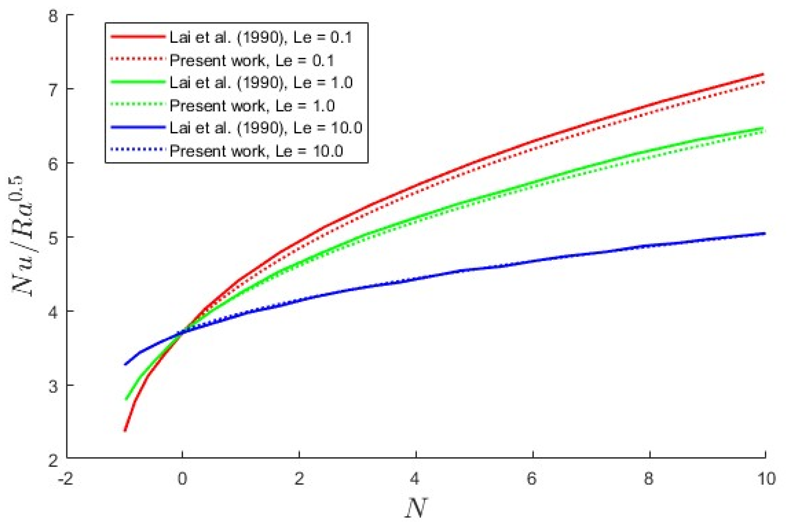
Before presenting the results, the numerical methodology employed in this study has been validated by comparing the results with canonical data reported by Lai et al. [28] on coupled heat and mass transfer in porous media. Specifically, Figure 2 presents a comparison of the Nusselt number (Nu) as a function of the buoyancy ratio (N) for three different Lewis numbers: Le = 0.1, 1.0, and 10.0. The results from the present numerical solution, obtained using MATLAB’s bvp4c solver, show excellent agreement with the benchmark data, capturing the trends and magnitudes across the entire range of N. This comparison demonstrates the capability of the current solver to handle coupled thermal and concentration gradients in porous media with high accuracy. The close alignment of results validates the robustness and reliability of our numerical approach and reinforces its applicability to the complex mixed convection flow considered in this study.

Figure 2.
The comparison of heat transfer results of Lai et al. [28] as a function of the buoyancy ratio for the cylinder.
4.1. Analysis of Velocity Profile
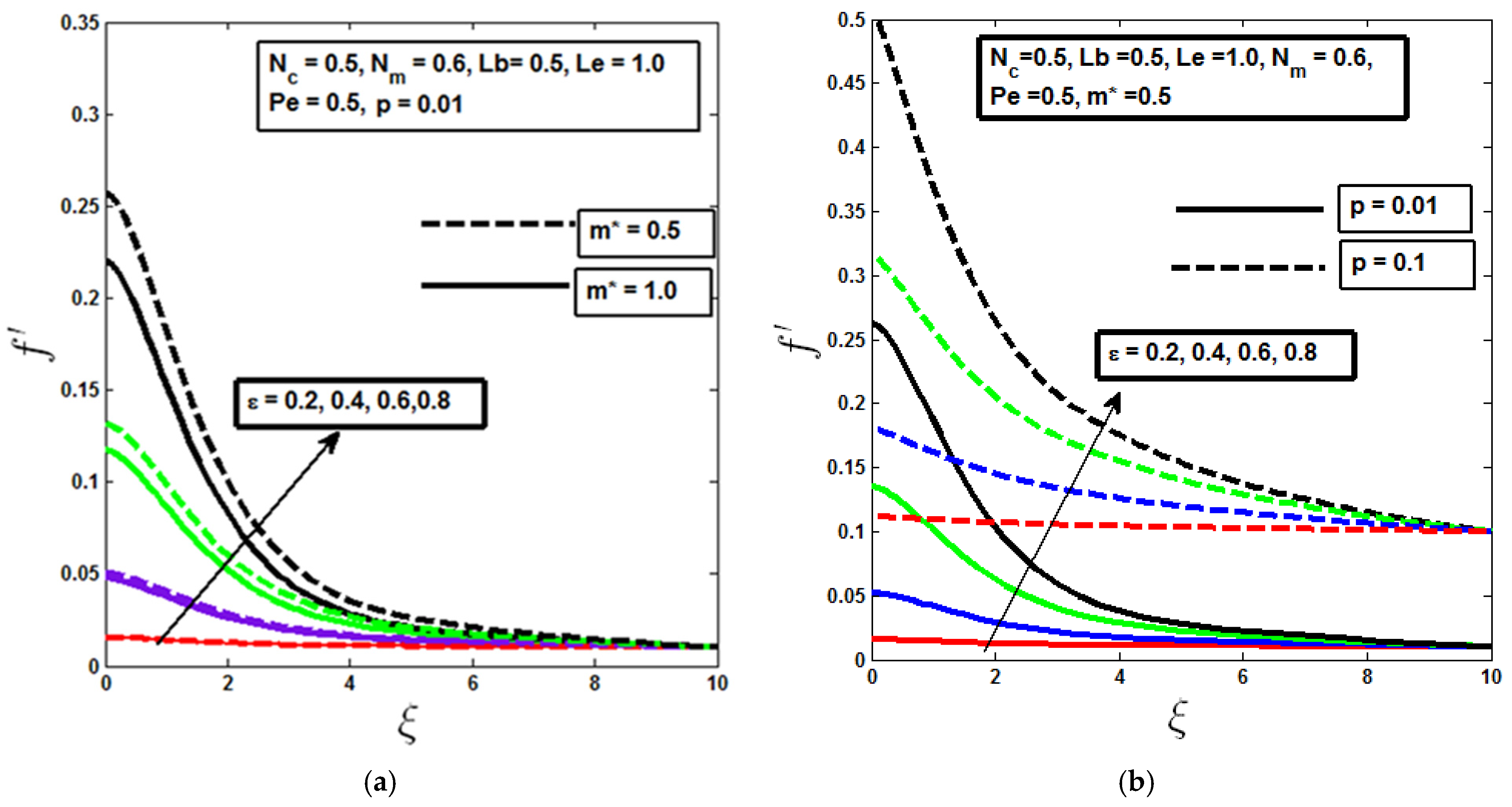
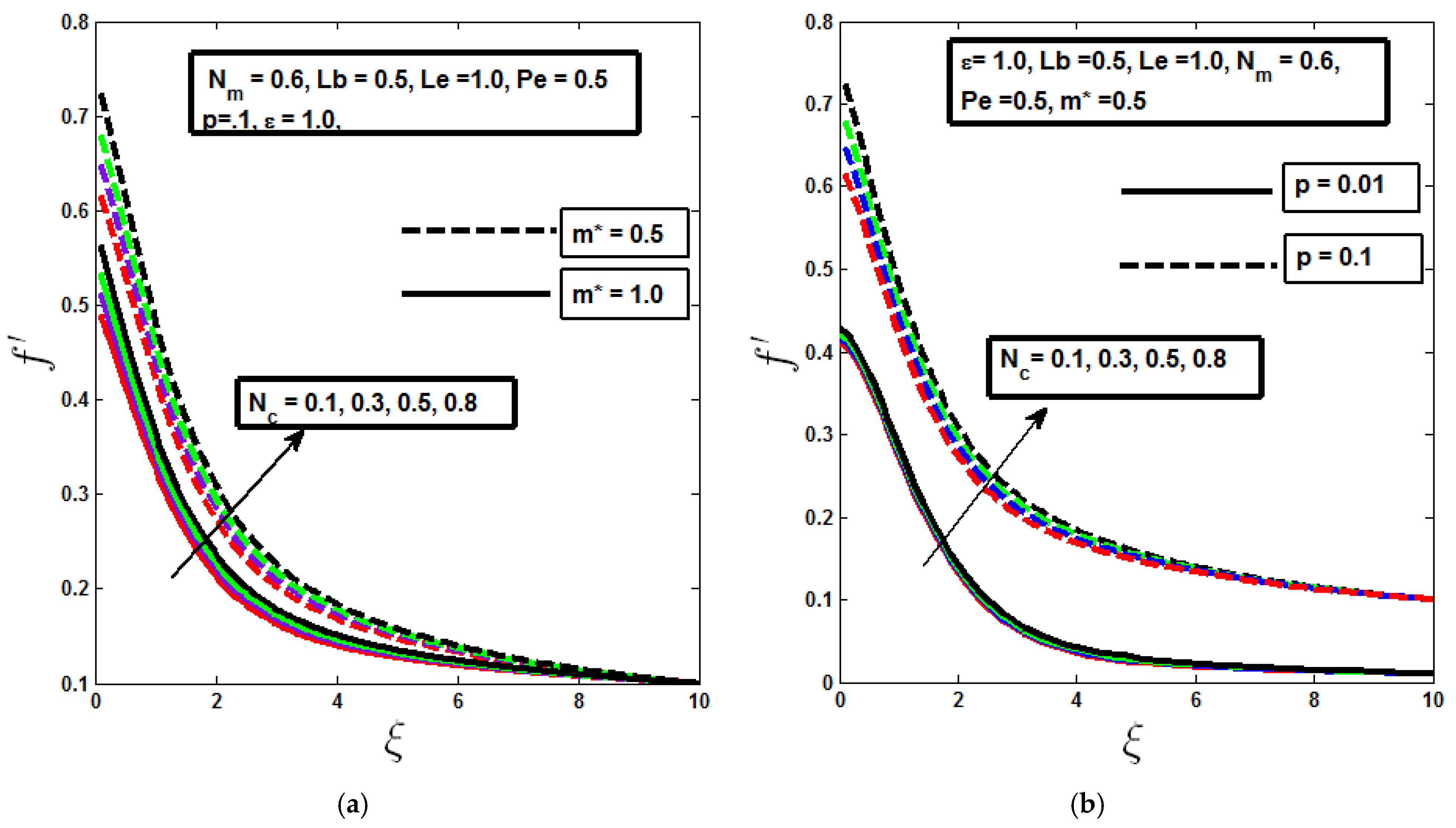
Figure 3 and Figure 4 show the distribution of the velocity profile for various values of the buoyancy parameter and the mixed convection parameter . In both isothermal (m* = 0.5) and non-isothermal (m* = 1.0) needle scenarios, as shown in Figure 3a and Figure 4a, and across different needle sizes, as depicted in Figure 3b and Figure 4b, the velocity profile increases as the values of and rise. This increase is driven by the buoyant forces that enhance fluid motion. When the mixed convection parameter is closer to zero, it indicates that the flow is primarily dominated by forced convection, where external forces, such as a pump or an imposed velocity, mainly drive the fluid motion. In this regime, the effects of buoyancy are minimal, and the velocity profiles reflect the influence of these external forces. As the mixed convection parameter increases, it signifies a transition towards a combined free and forced convection regime. In this context, buoyancy forces begin to play a more significant role, enhancing the overall fluid motion and leading to more pronounced velocity profiles.

Figure 3.
Change in velocity profile with mixed convection parameter for (a) different m* values and (b) varied needle diameters. [different color lines indicate change of from 0.2 to 0.8, along the arrow].

Figure 4.
Buoyancy parameter fluctuates with velocity distribution for (a) varying m* values and (b) various needle diameters. [different color lines indicate change of from 0.1 to 0.8, along the arrow].
The velocity boundary layer becomes thicker when using an isothermal needle compared to a non-isothermal one, and increasing the needle thickness further improves the velocity profile. This enhanced flow profile is due to momentum diffusion, facilitated by the needle’s larger contact area with the fluid. On the other hand, as the needle size decreases, a lesser proportion of its surface interacts with the fluid particles, leading to restricted fluid flow due to the frictional forces acting on the needle surface. In practical applications, this insight is particularly useful in fields such as chemical processing or biomedical engineering, where controlling fluid flow around needles or similar structures is crucial. For example, optimizing needle size and the buoyancy effects can enhance the efficiency of processes like drug delivery or heat exchangers, where precise control overflow profiles are necessary for optimal performance.
4.2. Analysis of Temperature Profile
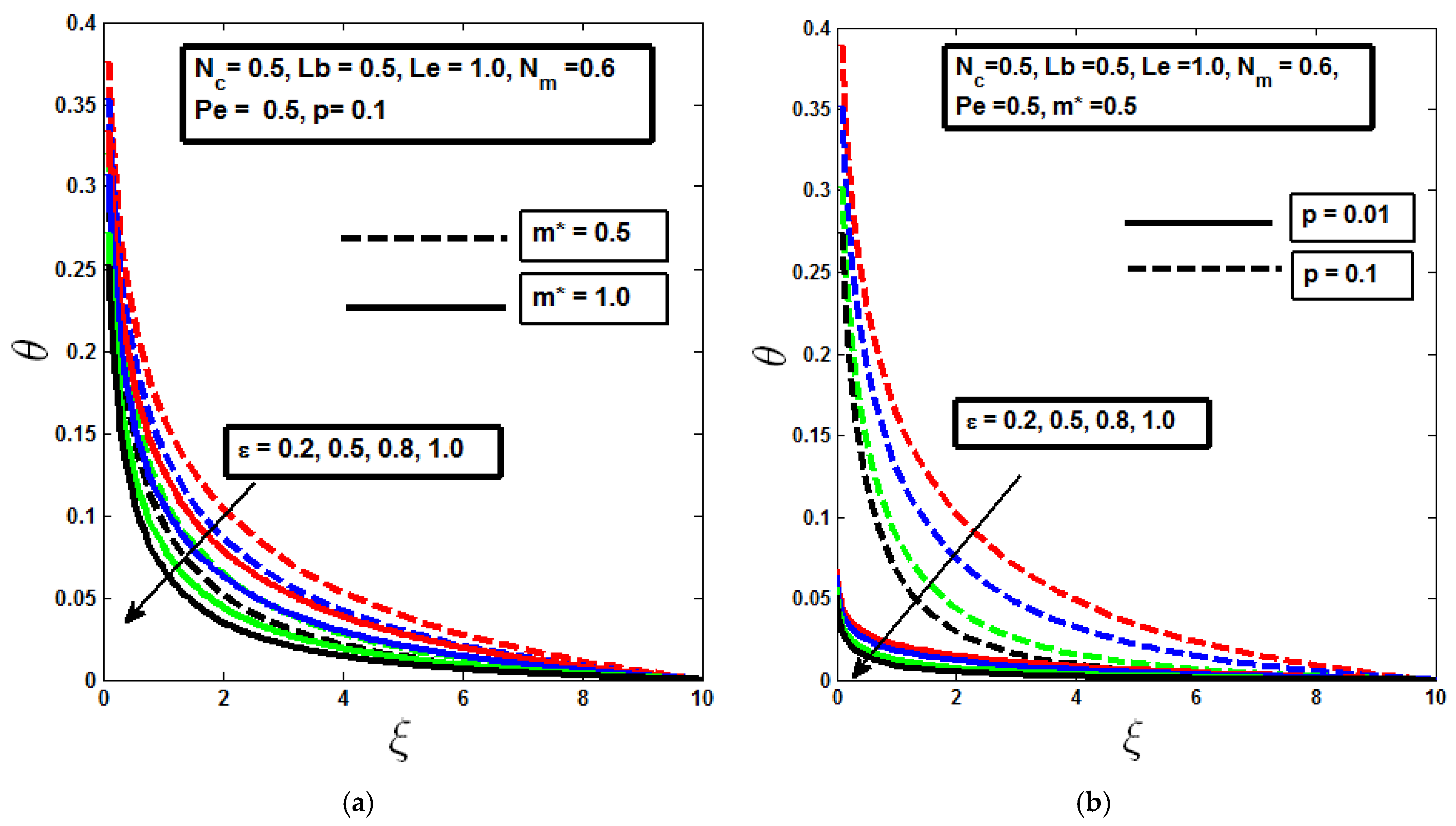
A decrease in the temperature profile with an increase in the mixed convection parameter and buoyancy parameter is observed in Figure 5a and Figure 6a, particularly for the non-isothermal needle (m* = 1.0), reflecting the complex interplay between forced and buoyant flows. As the mixed convection parameter increases, the influence of buoyancy forces becomes more significant, promoting upward flow that enhances cooling effects around the needle. This contrasts with the velocity profile, which may exhibit different dynamics due to the competing effects of momentum and thermal diffusion. When the needle thickness increases, it results in a thicker thermal boundary layer, which means that heat has a greater distance to diffuse before reaching the bulk fluid. This leads to lowering the temperature at the needle’s surface, as illustrated in Figure 5b and Figure 6b. The thicker boundary layer not only reduces the temperature gradient at the surface but also contributes to enhanced heat retention in the fluid immediately adjacent to the needle.

Figure 5.
Effect of mixed convection parameter on temperature profile for (a) different values of m* and (b) different needle sizes. [different color lines indicate change of from 0.2 to 1.0, along the arrow].

Figure 6.
Effect of buoyancy parameter on temperature profile for (a) different values of m* and (b) different needle sizes. [different color lines indicate change of from 0.2 to 0.8, along the arrow].
Furthermore, the interplay between momentum and thermal diffusion plays a crucial role in this context. A higher rate of momentum diffusion, driven by increased fluid flow, can impede the ability of heat to diffuse away from the needle surface, causing the cooling effect observed in the boundary layer. As a result, the thermal boundary layer becomes cooler and thinner, as supported by reference [15]. This phenomenon emphasizes the importance of considering both thermal and fluid dynamic factors when analyzing heat transfer processes in systems involving mixed convection, particularly when optimizing conditions for applications such as cooling or heating in biomedical and industrial settings.
In practical terms, this understanding is crucial in industries where precise thermal management is needed, such as designing cooling systems for microelectronics or biomedical applications where controlled temperature profiles around needles are critical. By optimizing the mixed convection parameter and needle geometry, engineers can effectively manage heat transfer to maintain optimal operating conditions or enhance the performance of thermal systems.
4.3. Analysis of Concentration Profile
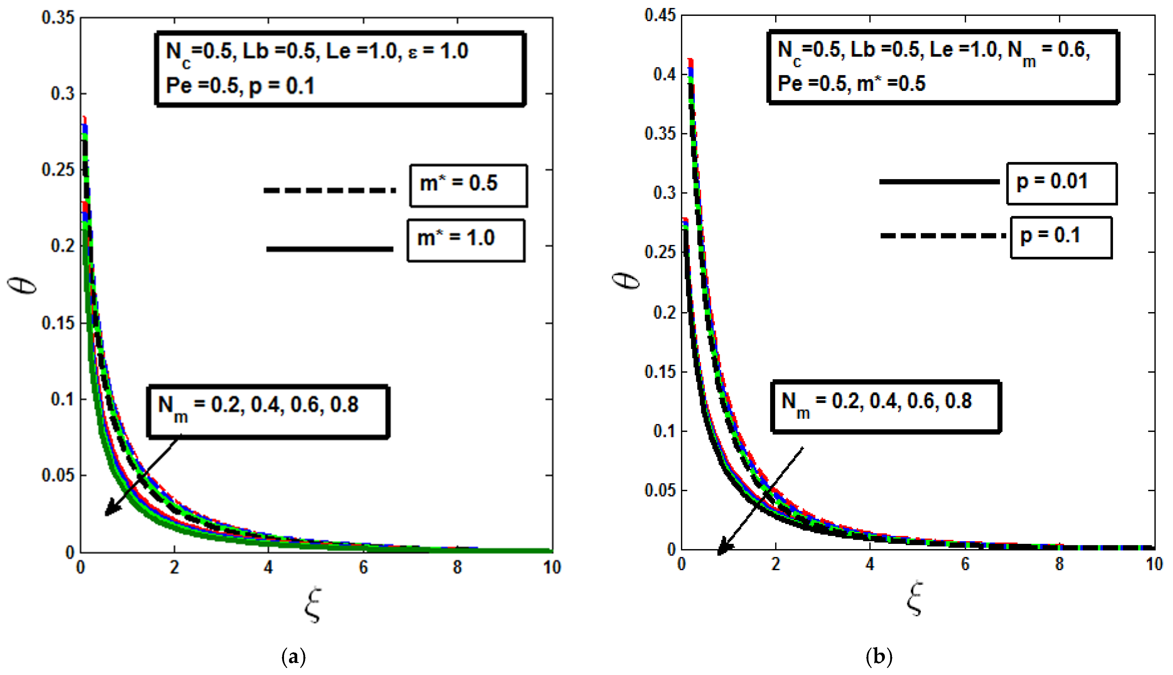
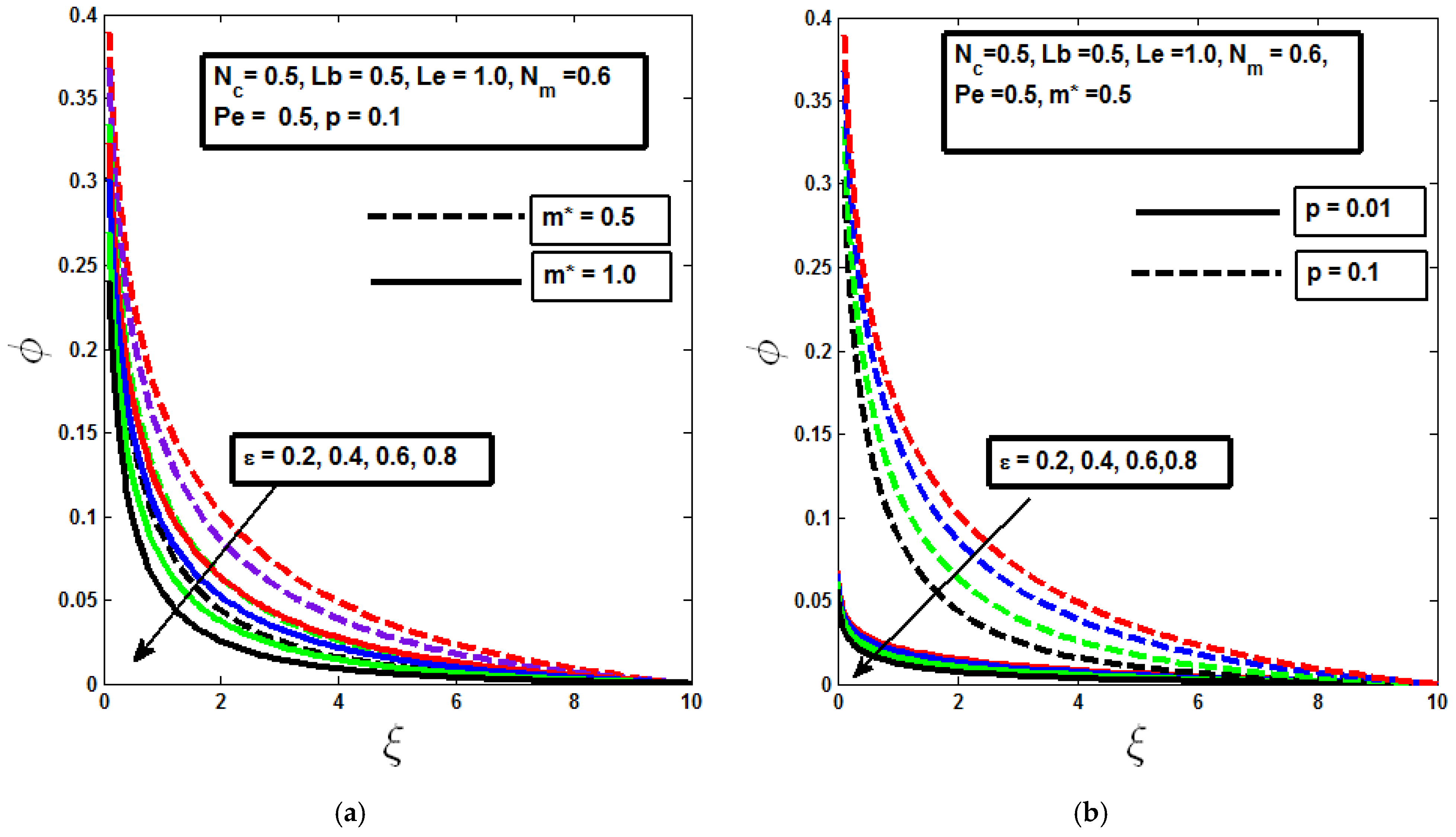
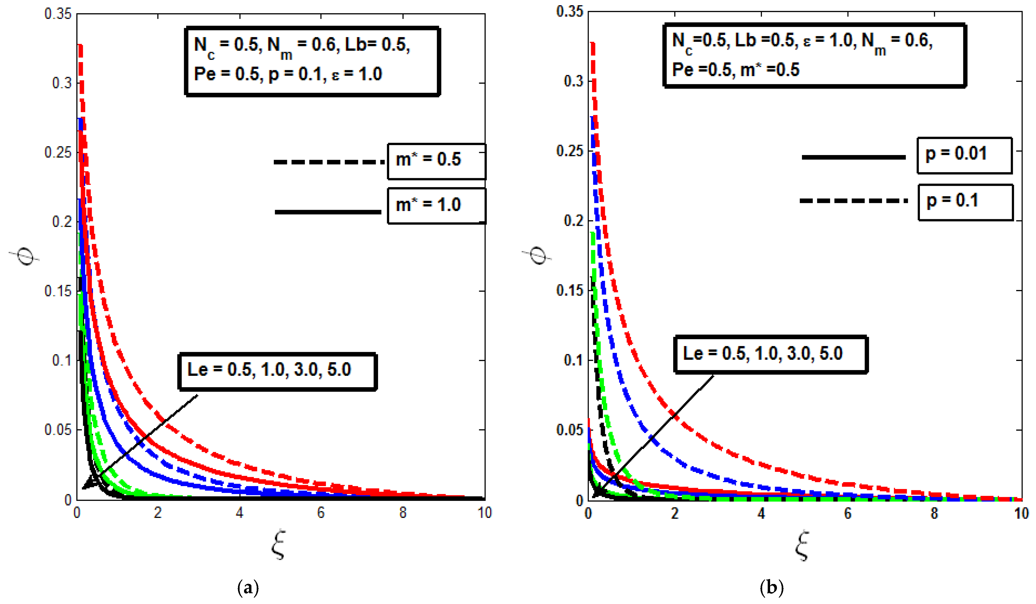
A decrease in the concentration profile with increasing mixed convection and Lewis number is observed in Figure 7a and Figure 8a, particularly in the non-isothermal case (m* = 1), which has important physical implications for heat and mass transfer dynamics around the slender needle. The Lewis number, the ratio of thermal diffusivity to mass diffusivity, indicates the relative rates of heat and mass transport. A higher suggests that heat diffuses more rapidly than mass, which alters the concentration distribution of the microorganisms in the vicinity of the needle. In the context of the non-isothermal needle, where temperature gradients are present, this enhanced thermal diffusivity leads to more effective heat transfer, creating a steeper temperature gradient that influences the movement of microorganisms. As increases, the concentration boundary layer becomes thinner, indicating that mass transfer is becoming more efficient relative to heat transfer. This results in a more pronounced reduction in the concentration profile, as shown in Figure 7b, due to the slender nature of the needle, which exacerbates the effects of heat on the mass distribution.

Figure 7.
Concentration profile with variation in mixed convection parameter for (a) different values of m* and (b) different needle sizes. [different color lines indicate change of from 0.2 to 0.8, along the arrow].

Figure 8.
Concentration profile with variation in Lewis parameter for (a) different values of m* and (b) different needle sizes. [different color lines indicate change of from 0.5 to 5.0, along the arrow].
Overall, the diminishing boundary layer thickness for both isothermal and non-isothermal configurations, illustrated in Figure 8b, underscores the interplay between heat and mass transfer processes. This phenomenon highlights the importance of carefully considering the Lewis number in the design and analysis of systems involving microbial transport, as it significantly impacts the concentration of microorganisms near the heat source, ultimately influencing their behaviour and distribution in fluid environments. In practical applications, such as in the design of biosensors or microfluidic devices, understanding how the Lewis number and needle geometry affect microbial flow is essential. For instance, in scenarios where the precise control of microbial concentration is required, optimizing the needle’s slenderness and adjusting the Lewis number can be vital in achieving desired outcomes in processes involving heat and mass transfer.
4.4. Analysis of Microorganism Profile
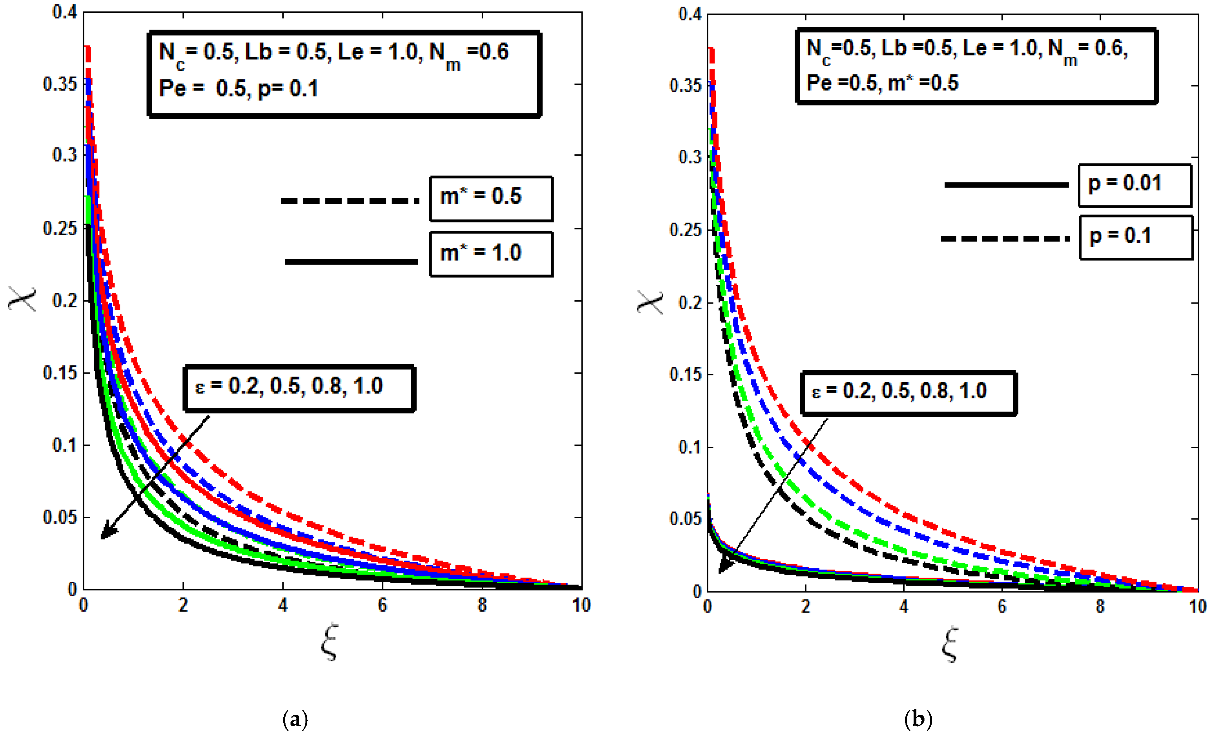
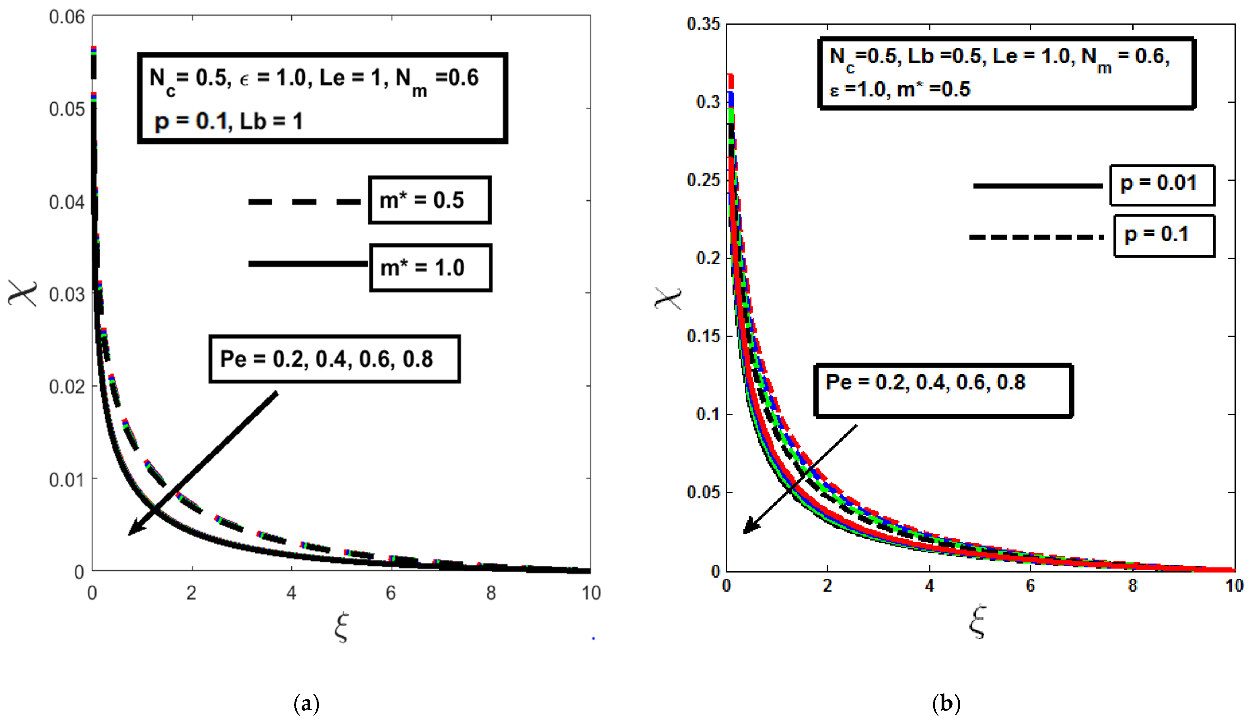
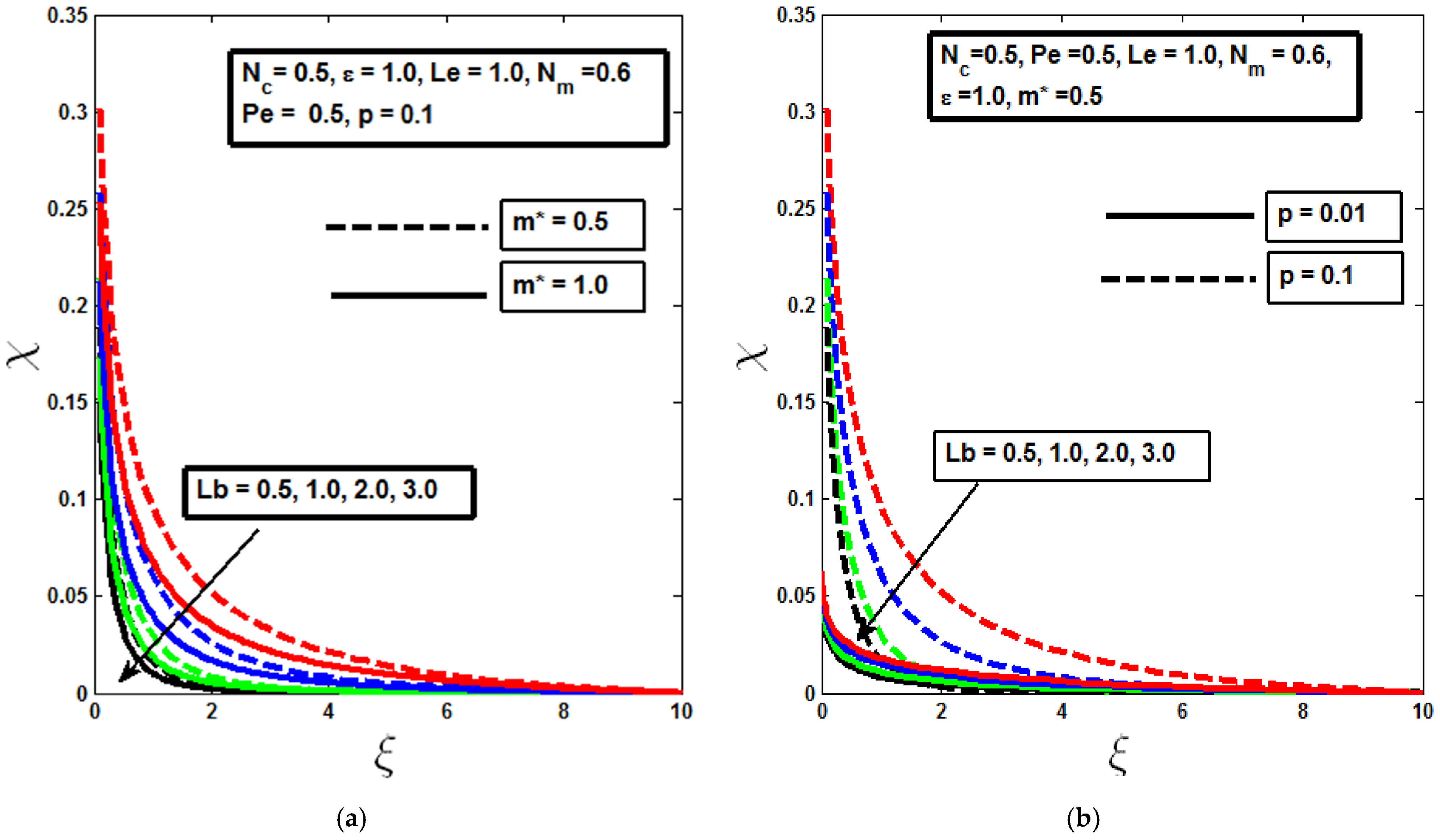
The results depicted in Figure 9, Figure 10 and Figure 11 highlight the complex interactions between various dimensionless parameters and the behaviour of motile microorganisms around the vertical thin needle. In Figure 9a, Figure 10a and Figure 11a, as the mixed convection parameter, Bioconvection Lewis number, and Bioconvection Peclet number increase, the observed reduction in microorganism profiles indicates that enhanced fluid mobility significantly affects microbial distribution. The increase in these parameters facilitates a more vigorous fluid flow, effectively redistributing motile microorganisms, and leading to a thinning of the microbial layer. This thinning effect is consistent across both isothermal (m* = 0.5) and non-isothermal (m* = 1.0) conditions, suggesting that the underlying dynamics are robust across different thermal scenarios.

Figure 9.
Microorganism profile with variation in mixed convection parameter for (a) different values of m* and (b) different needle sizes. [different color lines indicate change of from 0.2 to 1.0, along the arrow].

Figure 10.
Microorganism profile with variation in Bioconvection Peclet number for (a) different values of m* and (b) different needle sizes. [different color lines indicate change of from 0.2 to 0.8, along the arrow].
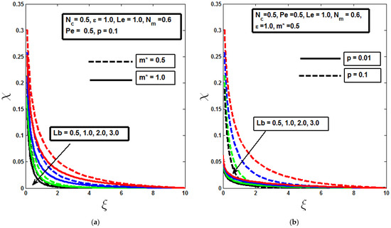
Figure 11.
Microorganism profile with variation Bioconvection Lewis parameter for (a) different values of m* and (b) different needle sizes. [different color lines indicate change of from 0.5 to 3.0, along the arrow].
Moreover, Figure 9b, Figure 10b and Figure 11b demonstrate that reducing the diameter of the needle further contributes to a thinner boundary layer in the microorganism profile. A smaller needle size increases the surrounding fluid’s velocity, which enhances motile microorganisms’ transport. This accelerated transport results in a diminished boundary layer thickness, as microorganisms are swept away more efficiently by the flow, reducing their local concentration near the needle surface. This practical insight is particularly relevant in applications where controlling the thickness of microbial layers is critical, such as in bioengineering processes or designing efficient cooling systems where microbial presence must be minimized.
4.5. Analysis of Surface Heat, Concentration, and Motile Microorganism Density
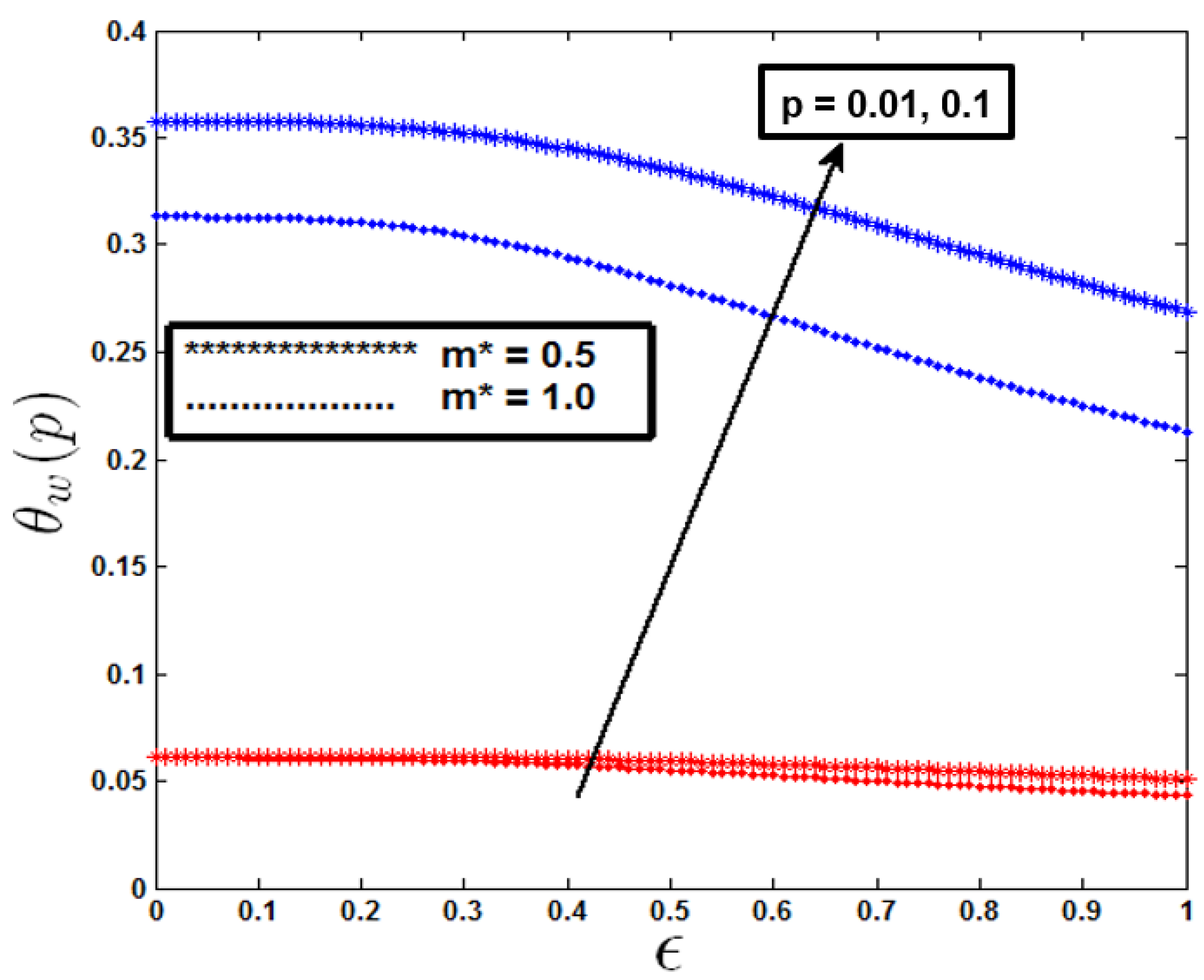
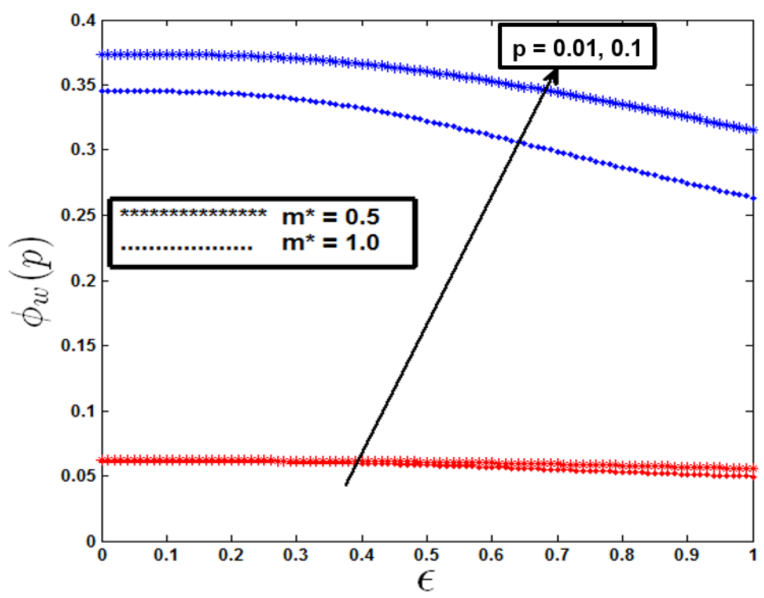
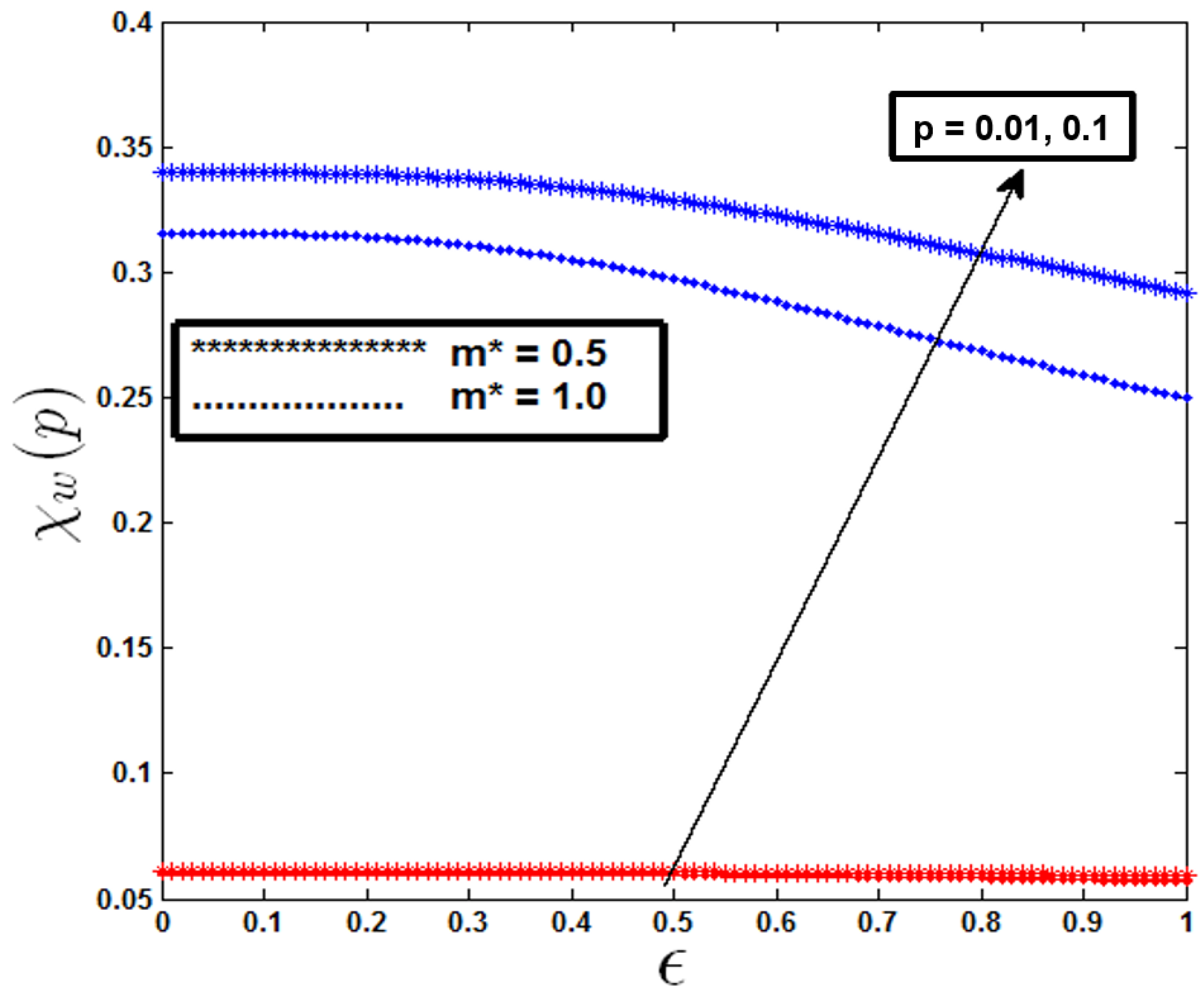
The observations presented in Figure 12, Figure 13 and Figure 14 illustrate the significant impact of the mixed convection parameter on surface temperature, fluid concentration, and motile microbe density. As increases, the corresponding decrease in surface temperature reflects the enhanced cooling effect driven by a combination of forced and buoyant flows. This cooling is more pronounced in non-isothermal conditions, where the temperature gradient around the needle intensifies, facilitating greater heat transfer away from the surface. The reduction in fluid concentration and motile microbe density, along with the drop in surface temperature, highlights the interconnected nature of thermal and microbial dynamics. As the mixed convection parameter increases, the enhanced fluid motion not only transports heat away from the surface but also disrupts the local concentration of motile microorganisms. This leads to a more effective dispersion of microbes into the bulk fluid, resulting in a lower density of microorganisms near the needle.

Figure 12.
Variation in surface temperature with mixed convection parameter . [red and blue refer to p = 0.01 and 0.1, respectively].

Figure 13.
Variation in surface fluid concentration with mixed convection parameter . [red and blue refer to p = 0.01 and 0.1, respectively].

Figure 14.
Variation in surface motile microorganism concentration with mixed convection parameter . [red and blue refers to p = 0.01 and 0.1, respectively].
The use of a slender needle further exacerbates this effect. Slender geometry increases the surface area-to-volume ratio, promoting more effective heat transfer and consequently lowering wall temperatures. Additionally, the reduced diameter accelerates the flow velocity around the needle, enhancing the transport of both heat and microorganisms. This results in an even greater dilution of motile microorganisms in the fluid, as they are swept away from the needle surface more efficiently. This understanding is vital for optimizing operations where temperature and concentration control are critical, such as biomedical devices or chemical reactors. For example, by modifying the mixed convection parameter and needle geometry, these systems can be fine-tuned to accomplish desired outcomes, such as increasing the efficiency of cooling mechanisms or improving the precision of microbial growth control in bioreactors.
5. Conclusions
This study provides a theoretical and numerical investigation of mixed convection flow around a vertical thin needle, integrating the dynamics of gyrotactic microorganisms under variable surface heat, mass, and microbial flux conditions. The analysis highlights the significant influence of dimensionless parameters such as mixed convection, buoyancy, and Bioconvection Lewis and Peclet numbers on velocity, temperature, concentration, and microorganism profiles. The findings reveal that increasing the mixed convection parameter enhances velocity profiles while reducing temperature, concentration, and microorganism profiles. Similarly, buoyancy parameters increase fluid velocity while suppressing the temperature gradient. It also demonstrates that slender needle geometries amplify fluid motion and heat transfer efficiency, leading to reduced thermal and microbial boundary layer thickness. These results have practical implications for optimizing heat and mass transfer processes in applications ranging from biomedical devices to industrial cooling systems. Furthermore, the study underscores the critical role of gyrotactic microorganisms in bioconvective systems, which can be leveraged to enhance fluid transport and nutrient mixing in bioengineering applications.
Future research should focus on the experimental validation of these findings to further establish their applicability in real-world scenarios. Additionally, extending the current framework to include unsteady flows, non-Newtonian fluids, or anisotropic porous media could provide deeper insights. Practical applications may also be influenced by factors such as turbulence transition and surface roughness. These factors may alter microorganism behaviour, increase energy losses, and modify buoyancy and drag forces. A comprehensive understanding of these effects is essential for optimizing the performance of systems utilizing mixed convection flows around thin needles.
Author Contributions
Conceptualization, N.I.N. and M.A.H.; methodology, N.I.N.; software, N.I.N.; validation, M.A.H.; formal analysis, N.I.N.; investigation, N.I.N.; resources, N.I.N.; data curation, M.A.H.; writing—original draft preparation, N.I.N.; writing—review and editing, M.A.H.; visualization, N.I.N.; supervision, M.A.H. project administration, M.A.H. funding acquisition, M.A.H. All authors have read and agreed to the published version of the manuscript.
Funding
This research received no external funding.
Data Availability Statement
The raw data supporting the conclusions of this article will be made available by the authors on request.
Conflicts of Interest
The authors declare no conflict of interest.
References
- Nasir, N.A.A.M.; Ishak, A.; Pop, I. Stagnation-point flow and heat transfer past a permeable quadratically stretching/shrinking sheet. Chin. J. Phys. 2017, 55, 2081–2091. [Google Scholar] [CrossRef]
- Aly, A.M.; Raizah, Z.A.S. Mixed convection in an inclined nanofluid filled-cavity saturated with a partially layered porous medium. J. Therm. Sci. Eng. Appl. 2019, 11, 041002. [Google Scholar] [CrossRef]
- Rashid, A.; Ayaz, M.; Islam, S. Numerical investigation of the magnetohydrodynamic hybrid nanofluid flow over a stretching surface with mixed convection: A case of strong suction. Adv. Mech. Eng. 2023, 15, 16878132231179616. [Google Scholar] [CrossRef]
- Raju, B.H.S.; Nath, D.; Pati, S.; Baranyi, L. Analysis of mixed convective heat transfer from a sphere with an aligned magnetic field. Int. J. Heat Mass Transf. 2020, 162, 120342. [Google Scholar] [CrossRef]
- Ahmad, U.; Ashraf, M.; Abbas, A.; Rashad, A.M.; Nabwey, H.A. Mixed convection flow along a curved surface in the presence of exothermic catalytic chemical reaction. Sci. Rep. 2021, 11, 12907. [Google Scholar] [CrossRef] [PubMed]
- Ahmed, K.; Akbar, T.; Ahmed, I.; Muhammad, T.; Amjad, M. Mixed convective MHD flow of Williamson fluid over a nonlinear stretching curved surface with variable thermal conductivity and activation energy. Numer. Heat Transf. Part A Appl. 2023, 85, 942–957. [Google Scholar] [CrossRef]
- Everts, M.; Mahdavi, M.; Meyer, J.P.; Sharifpur, M. Development of the hydrodynamic and thermal boundary layers of forced convective laminar flow through a horizontal tube with a constant heat flux. Int. J. Therm. Sci. 2023, 186, 108098. [Google Scholar] [CrossRef]
- Khan, W.A.; Rashad, A.M.; Abdou, M.M.M.; Tlili, I. Natural bioconvection flow of a nanofluid containing gyrotactic microorganisms about a truncated cone. Eur. J. Mech.-B/Fluids 2019, 75, 133–142. [Google Scholar] [CrossRef]
- Saleem, S.; Rafiq, H.; Al-Qahtani, A.; El-Aziz, M.A.; Malik, M.Y.; Animasaun, I.L. Magneto Jeffrey nanofluid bioconvection over a rotating vertical cone due to gyrotactic microorganism. Math. Probl. Eng. 2019, 2019, 3478037. [Google Scholar] [CrossRef]
- Mahdy, A.; Nabwey, H.A. Microorganisms time-mixed convection nanofluid flow by the stagnation domain of an impulsively rotating sphere due to Newtonian heating. Results Phys. 2020, 19, 103347. [Google Scholar] [CrossRef]
- Sudhagar, P.; Kameswaran, P.K.; Kumar, B.R. Gyrotactic microorganism effects on mixed convective nanofluid flow past a vertical cylinder. J. Therm. Sci. Eng. Appl. 2019, 11, 041018. [Google Scholar] [CrossRef]
- Mallikarjuna, B.; Rashad, A.M.; Chamkha, A.; Abdou, M.M.M. Mixed bioconvection flow of a nanofluid containing gyrotactic microorganisms past a vertical slender cylinder. Front. Heat Mass Transf. (FHMT) 2018, 10, 1–8. [Google Scholar] [CrossRef]
- Rashad, A.M.; Nabwey, H.A. Gyrotactic mixed bioconvection flow of a nanofluid past a circular cylinder with convective boundary condition. J. Taiwan Inst. Chem. Eng. 2019, 99, 9–17. [Google Scholar] [CrossRef]
- Mahdy, A. Unsteady Mixed Bioconvection Flow of Eyring–Powell Nanofluid with Motile Gyrotactic Microorganisms Past Stretching Surface. BioNanoScience 2021, 11, 295–305. [Google Scholar] [CrossRef]
- Waqas, H.; Manzoor, U.; Shah, Z.; Arif, M.; Shutaywi, M. Magneto-burgers nanofluid stratified flow with swimming motile microorganisms and dual variables conductivity configured by a stretching cylinder/plate. Math. Probl. Eng. 2021, 2021, 8817435. [Google Scholar] [CrossRef]
- Bilal, S.; Rehman, K.U.; Shatanawi, W.; Shflot, A.S.; Malik, M.Y. Heat Transfer Analysis of Carreau Nanofluid Flow with Gyrotactic Microorganisms: A Comparative Study. Case Stud. Therm. Eng. 2024, 60, 104617. [Google Scholar] [CrossRef]
- Alharbi, K.A.M.; Bilal, M.; Ali, A.; Eldin, S.M.; Alburaikan, A.; Khalifa, H.A.E.W. Significance of gyrotactic microorganisms on the MHD tangent hyperbolic nanofluid flow across an elastic slender surface: Numerical analysis. Nanotechnol. Rev. 2023, 12, 20230106. [Google Scholar] [CrossRef]
- Alam, M.M.; Arshad, M.; Alharbi, F.M.; Hassan, A.; Haider, Q.; Al-Essa, L.A.; Eldin, S.M.; Saeed, A.M.; Galal, A.M. Comparative dynamics of mixed convection heat transfer under thermal radiation effect with porous medium flow over dual stretched surface. Sci. Rep. 2023, 13, 12827. [Google Scholar] [CrossRef]
- Khan, Z.; Thabet, E.N.; Habib, S.; Abd-Alla, A.M.; Bayones, F.S.; Alharbi, F.M.; Alwabli, A.S. Numerical study of hydromagnetic bioconvection flow of micropolar nanofluid past an inclined stretching sheet in a porous medium with gyrotactic microorganism. J. Comput. Sci. 2024, 78, 102256. [Google Scholar] [CrossRef]
- Yasmin, H. Numerical investigation of heat and mass transfer study on MHD rotatory hybrid nanofluid flow over a stretching sheet with gyrotactic microorganisms. Ain Shams Eng. J. 2024, 15, 102918. [Google Scholar] [CrossRef]
- Beg, O.A.; Zohra, F.T.; Uddin, M.J.; Ismail, A.I.M.; Sathasivam, S. Energy conservation of nanofluids from a biomagnetic needle in the presence of Stefan blowing: Lie symmetry and numerical simulation. Case Stud. Therm. Eng. 2021, 24, 100861. [Google Scholar]
- Grosan, T.; Pop, I. Forced convection boundary layer flow past non-isothermal thin needles in nanofluids. J. Heat Transfer. 2011, 133, 054503. [Google Scholar] [CrossRef]
- Soid, S.K.; Ishak, A.; Pop, I. Boundary layer flow past a continuously moving thin needle in a nanofluid. Appl. Therm. Eng. 2017, 114, 58–64. [Google Scholar] [CrossRef]
- Hayat, T.; Khan, M.I.; Farooq, M.; Yasmeen, T.; Alsaedi, A. Water-carbon nanofluid flow with variable heat flux by a thin needle. J. Mol. Liq. 2016, 224, 786–791. [Google Scholar] [CrossRef]
- Ali, B.; Jubair, S.; Al-Essa, L.A.; Mahmood, Z.; Al-Bossly, A.; Alduais, F.S. Boundary layer and heat transfer analysis of mixed convective nanofluid flow capturing the aspects of nanoparticles over a needle. Mater. Today Commun. 2023, 35, 106253. [Google Scholar] [CrossRef]
- Salleh, S.N.A.; Bachok, N.; Arifin, N.M.; Ali, F.M. Influence of Soret and Dufour on forced convection flow towards a moving thin needle considering Buongiorno’s nanofluid model. Alex. Eng. J. 2020, 59, 3897–3906. [Google Scholar] [CrossRef]
- Waini, I.; Ishak, A.; Pop, I. Hybrid nanofluid flow past a permeable moving thin needle. Mathematics 2020, 8, 612. [Google Scholar] [CrossRef]
- Lai, F.C.; Choi, C.Y.; Kulacki, F.A. Coupled heat and mass transfer by natural convection from slender bodies of revolution in porous media. Int. Commun. Heat Mass Transf. 1990, 17, 609–620. [Google Scholar] [CrossRef]
Disclaimer/Publisher’s Note: The statements, opinions and data contained in all publications are solely those of the individual author(s) and contributor(s) and not of MDPI and/or the editor(s). MDPI and/or the editor(s) disclaim responsibility for any injury to people or property resulting from any ideas, methods, instructions or products referred to in the content. |
© 2025 by the authors. Licensee MDPI, Basel, Switzerland. This article is an open access article distributed under the terms and conditions of the Creative Commons Attribution (CC BY) license (https://creativecommons.org/licenses/by/4.0/).