Longitudinal Dispersion and Hyporheic Exchange of Neutrally Buoyant Microplastics in the Presence of Waves and Currents

Abstract

An experimental study was conducted to identify the behaviour of neutrally buoyant microplastics (specific density, 0.94) in different hydrodynamic conditions while focusing on combined wave–current conditions and the mixing across the hyporheic zone. For in-water-column microplastics, it was observed that the streamwise dispersion of neutrally buoyant microplastics is comparable to solute dye in both slow open-channel flow conditions and combined wave–current conditions. However, for in-bed microplastics, when compared to soluble tracers, the longer timespans associated with the hyporheic exchange process allowed the density effects to enhance the vertical exchange when compared to solutes.

1. Introduction

Plastic debris with size less than 5 mm diameter are generally defined as “microplastics” [1,2]. These particles originate from various sources, including the direct manufacture of microbeads used in personal hygiene products [3,4,5,6] or from the breakdown of larger structures through physical contact, wear and tear, and weathering, such as car tyres [7], road markings, and synthetic plastic fibres in modern textiles. While conventional wastewater treatment practices often eliminate most microbeads, persistent microfiber plastics remain unfiltered, facilitating their undetected infiltration into marine environments [6]. Approximately 10% of produced plastics enter the oceans [8], contributing to an estimated 80–85% of marine litter. Within this litter, there is an estimated 5.25 trillion plastic particles (0.27 tons) in the ocean, with 92% of these being microplastics by number and 13% by weight [9], in addition to the plastics on the seabed [10] and beaches [11]. Recent studies have also found microplastics in the remotest of regions, including six of the deepest ecosystems on Earth as well as within sea ice in the Arctic [12]. Microplastics can attract various toxins and hydrophobic compounds [13] and accumulate in organisms [14], leading to the deterioration of aquaculture environments [15]. The presence of microplastics in food webs can cause adverse health effects [16].

Despite the significant amount of microplastics being swept into waterbodies, there is currently extremely limited literature available on the movement of microplastics in ponds, wetlands, and coastal areas under the influence of waves. Understanding the means of transport and removal of microplastics in benthic regions is beneficial in planning effective waste management systems, which helps mitigate the harmful impacts on human health and the diverse ecosystems. The mixing and spreading of soluble pollutants in various waterbodies can be explained relative to the hydrodynamics of water if the addition of pollutants does not alter the properties of water, such as the density and the viscosity [17]. However, the solute transport processes in complex hydrodynamic conditions as well as across the hyporheic zone is not fully understood, and the extra complexities introduced when microplastic mixing is being considered, with the added buoyancy effects [18], remain unknown. It is difficult to determine the movements of matter close to neutral buoyancy, as denser microplastics tend to sink, and lighter microplastics tend to wash ashore regularly [19]. There are similarities that govern the transport mechanisms of solutes and fine sediments in fluvial systems through means of diffusion and dispersion [20]. As such, it is possible that neutrally buoyant microplastics could mimic solute transport in natural environments. Polyethylene, one of the neutrally buoyant microplastics, with a specific density of 0.91–0.97 [21], exists abundantly in the natural environment.

In recent years, the methodology for the quantification of environmental microplastic contamination has been restricted due to a lack of methods sensitive enough to quantify the data. Commonly applied techniques included separating microplastics via density separation and identification via spectroscopy, from which the obtained data could provide a lower estimation of small microplastics due to the visual step in the process [22]. An alternative method that utilises the solute Nile red dye to increase the detection of small microplastic particles through fluorescence microscopy and image analysis software was presented by Erni-Cassola et al. [23]. This method was found to be inexpensive, employing readily available equipment, and can be semi-automated for high-throughput sample analysis without altering the material properties of microplastics such as the density. The method involves artificially staining the microplastics through chemically impregnating them with dye. This protocol has proven to be effective in the quantification of small polyethylene, polypropylene, polystyrene, and nylon-6 particles. The Nile red dye used by Erni-Cassola et al. [23] to stain their range of microplastics exhibited a fluorescence signature similar to that of Rhodamine WT solution, a commonly used fluorescent dye in tracer studies [24]. Rhodamine WT is a soluble dye in water, and if it is found to mimic the movement of microplastics in experimental lab conditions, then it could be used to further study microplastic movement in various natural environments [24]. This is significant, as Rhodamine WT has been used as a surrogate hazardous agent in multiple other studies due to its low environmental impact and ease of traceability [25]. The approach of chemically impregnating microplastics with Nile red dye has been used in laboratory settings, and it has been observed that the longitudinal dispersion properties of neutrally buoyant microplastics is comparable to solute Rhodamine WT dye in open-channel flow conditions with bare beds [24] as well as open-channel flows with submerged vegetation [26]. When microplastics with different densities were tested for their longitudinal dispersion properties, it was observed that the density started to dominate when the critical velocity was less than 0.1 m/s [27].

The aim of this study was to investigate the mixing properties of neutrally buoyant microplastics when the flow velocities are smaller than 0.1 m/s, allowing the density of the microplastics to affect the processes. Longitudinal mixing and mixing across the hyporheic zone were studied for slow open-channel flow conditions, which replicate ponds and wetlands, and waves propagating on slow background currents, which replicate wind and swell waves on slow tidal currents. Microplastic dispersion in combined wave–current conditions has not been studied in full, and the mixing across the hyporheic zone is a slow process that will allow the density of microplastics to dominate.

2. Theoretical Background

2.1. Longitudinal Dispersion Coefficient

The diffusion flux, i.e., the mass transport rate per a unit width per unit time $\dot{\left(M\right)}$ in the streamwise direction $\left(x\right)$, of an open channel is given by Equation (1):

$$\dot{M}=-hD{\displaystyle \frac{\partial \overline{C}}{\partial x}}$$

(1)

where $h$ is the water depth, and $\overline{C}$ is the depth averaged mean concentration. This is a depth-averaged model based on Fick’s first law [28]. $D$ is called the coefficient of longitudinal dispersion, denoting a bulk transport coefficient depending on the diffusive property of the velocity distribution of the flow. The magnitude of $D$ is a function of the flow properties. For an infinitely wide open-channel flow with a logarithmic velocity profile, the longitudinal dispersion coefficient $\left(D\right)$ is given by Equation (2):

$$D=5.93 h{u}_{\ast }$$

(2)

where $u_{\ast }$ is the friction velocity. The friction velocity is defined as shown in Equation (3):

$$u_{\ast }=\sqrt{{\displaystyle \frac{{\tau }_0}{\rho }}}$$

(3)

where ${\tau }_0$ is the bed shear stress of the channel, and $\rho$ is the fluid density.

The longitudinal dispersion coefficient can be experimentally calculated by measuring how a tracer cloud disperses when it travels downstream along a flow. Using measurement devices, the concentration time series of the tracer could be measured in several locations along the flow. The temporal variance of the concentration time series increases along the streamwise direction, and the rate of change of the variance can be converted into the longitudinal dispersion coefficient using Equation (4) [29,30]:

$$D={\displaystyle \frac{1}{2}}{\displaystyle \frac{d}{dt}}\left[{\stackrel{̿}{u}}^2{\sigma }_t^2\right]={\displaystyle \frac{{\stackrel{̿}{u}}^2}{2}}{\displaystyle \frac{{\sigma }_{t\left(x_2\right)}^2-{\sigma }_{t\left(x_1\right)}^2}{t_2-t_1}}$$

(4)

where ${\sigma }_t^2$ is the temporal variance of the tracer concentration time series measured at two different locations along the flow, and $\stackrel{̿}{u}$ is the average flow velocity. $t_1$ and $t_2$ denote the timesteps when the centroid of the solute cloud passes each location. In the laboratory, the average flow velocity can be estimated based on the time taken by the solute cloud to travel between two locations, which are located apart by a known distance.

2.2. Mixing in Porous Sediments across the Hyporheic Zone

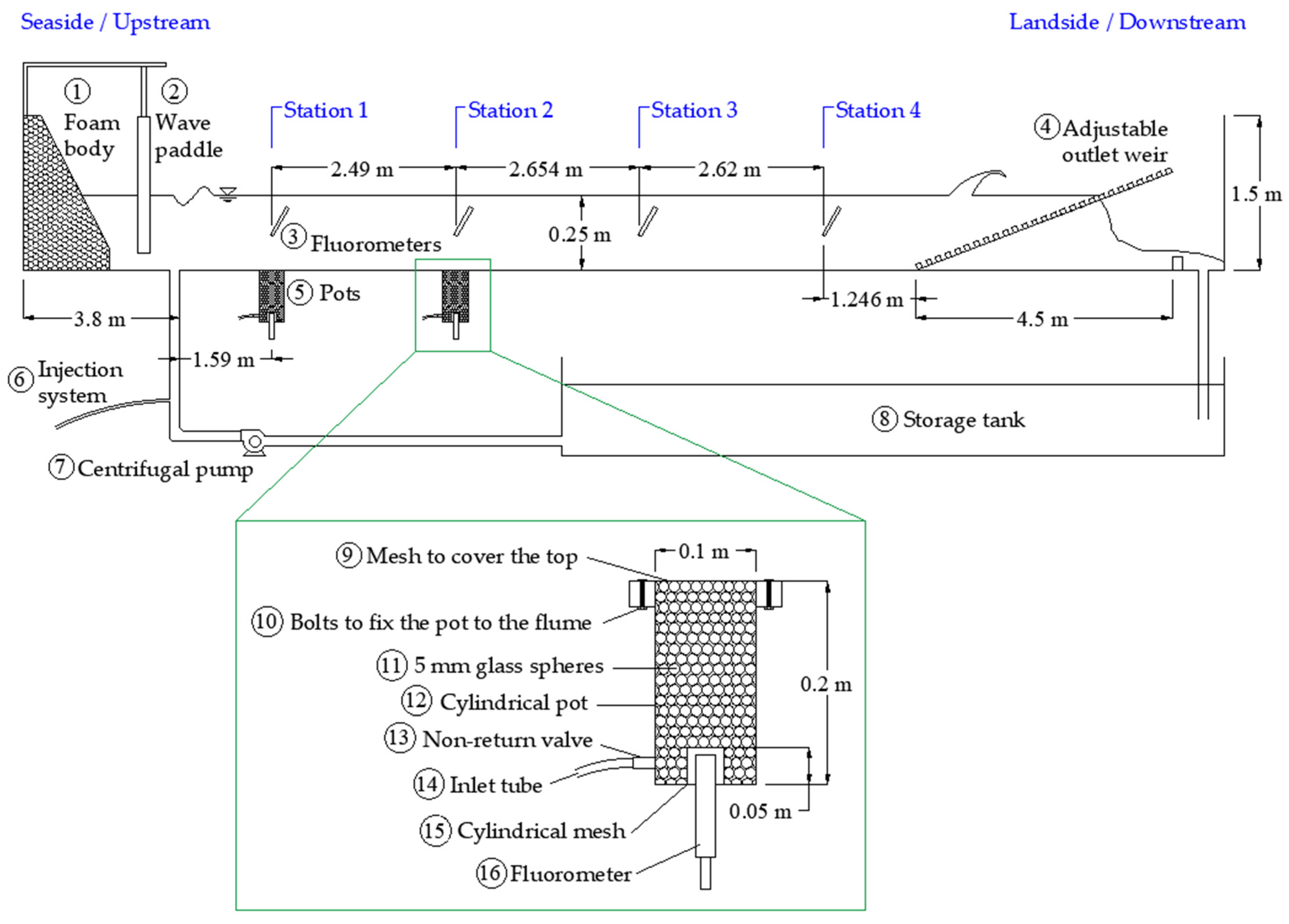
The mixing of solute beneath waterbodies was studied as two sub-sections: the movement of solute across the sediment–water interface and the movement of solute in bed. Studies about both processes use the same theoretical framework: Fick’s second law [28] in one dimension [31], which is shown in Equation (5):

$${\displaystyle \frac{\partial C}{\partial t}}=D_m{\displaystyle \frac{{\partial }^{2}C}{\partial z^2}}$$

(5)

where $D_m$ is the vertical mixing coefficient inside the bed.

By using a modified erosimeter, Chandler et al. (2016) [31] established two scaling relationships for interface exchange and in-bed mixing. The scaling relationship for interface exchange is given by Equation (6), and the in-bed mixing coefficient is shown in Equation (7):

$${\displaystyle \frac{D_e}{D_m^{\prime }}}=3.38\times {10}^{11}{d}_g^{2.1}{u}_{\ast }^{1.55}$$

(6)

$$D_m=1.19\times {10}^6{d}_g^{2.22}{u}_{\ast }^{3.11}{e}^{55z}$$

(7)

where $D_e$ is the effective interface exchange coefficient, $D_m^{\prime }$ is the molecular diffusion coefficient in sediment pore water, and $d_g$ is the geometric mean particle diameter of the bed sediment.

3. Methodology

3.1. Types of Tracers, Instrumentation, and Calibration

The solute dispersion was modelled using soluble Rhodamine WT dye, and the concentration was measured through its fluorescence as a proxy by using Cyclops-7 fluorometers (from Turner Designs, San Jose, CA, USA). To allow tracking microplastics using the same fluorometers, the microplastics (polyethylene: product number 434272 by Sigma-Aldrich, Burlington, MA, USA; particle size: 34–50 μm; density: 0.94 g/mL at 25 °C) were chemically impregnated with Nile red dye to add fluorescent properties.

The methodology of chemically impregnating microplastics with Nile red dye followed the work by Erni-Cassola et al. [23] and Cook et al. [24]. Before attaching the fluorometers in the flume setup, the fluorometers were calibrated to link the output voltages with the solute and microplastic concentrations. This was performed by submerging the fluorometers in four different solutions with known concentrations (0, 10, 20, and 40 PPB for Rhodamine WT and 0, 0.05, 0.10, and 0.20 g/L for microplastics) following the guidelines given by Turner Designs.

The experiments were carried out in a 20 m long, 0.34 m wide, and 1.5 m deep flume made of fibre-reinforced plastic. The flow was generated using a centrifugal pump, and the waves were created using a piston wave paddle (from HR Wallingford, Oxfordshire, UK). The definition of wave properties and the operation of the wave paddle was controlled through the HR Merlin software (from HR Wallingford, Oxfordshire, UK). The water depth was kept constant at 0.25 m. In the downstream end of the flume, an energy-dissipating weir with a 1:5 slope was installed. The weir had a series of holes in it to facilitate changing the flow rate while maintaining a constant water depth. The experimental setup is shown in Figure 1.

3.2. Longitudinal Dispersion Measurements

The soluble tracer sample was prepared using Rhodamine WT with a concentration of 100,000 PPB. The buoyant microplastic sample was prepared using polyethylene with a concentration of 20 g/L. The microplastic sample was stirred continuously until the injection was carried out to keep them suspended. To quantify longitudinal mixing along the flume, the tracers were injected to the inlet pipe for four seconds using a peristaltic pump with a flow rate of 40 mL/min. This signal was sent to the pump via an Arduino IDE, and the data collection was started 20 s before the injection was initiated to estimate the background concentration. The injection point was chosen in the inlet pipe so that the cross-sectional mixing was achievable by the time the tracer cloud entered the flume. The concentrations were measured using four fluorometers positioned in four stations along the flume, as shown in Figure 1. The fluorometers were mounted in mid-water depth with an inclination of 30 degrees to ensure additional clearance space and to reduce the formation of air bubbles around the sensor. The fluorometers were connected to a data acquisition device (USB-6009 by National Instruments, Austin, TX, USA) that logged the output voltages once every second and saved the data on the hard disk through a LABVIEW graphical user interface. The experiments were carried out until the tracers passed through the flume and the fluorometer readings returned to values closer to the initial readings.

3.3. Measuring Mixing across the Hyporheic Zone

To quantify mixing across the hyporheic zone, the hyporheic zone was modelled using cylindrical pots attached to the bottom of the flume. The pots were manufactured in the laboratory using PVC pipes, and the dimensions are shown in Figure 1. A closer view of a single pot is also shown in Figure 1. The pots were attached below the fluorometers in the same four stations as shown in Figure 1. The reason for using two pots along the flume was to obtain a repetition for each test condition. A fluorometer was attached to the bottom of each pot, and a cylindrically shaped mesh was fixed around the fluorometer, as shown in Figure 1. The size of the holes in the cylindrical mesh was chosen to be smaller than 5 mm (which is the size of glass spheres) to create a clear area around the fluorometer with no interruption from glass spheres, facilitating accurate concentration readings. The pots were filled with glass spheres up to the top, and the top surface was covered with a lid made by a stainless-steel mesh (with hole diameters slightly less than 5 mm) to keep the glass spheres in place without being washed away by the flow.

The centrifugal pump, which created the slow open-channel flow, was switched on, and the waterflow was left running for about an hour until a steady state was achieved. When the water depth became consistent at 0.25 m for the given flow rate, the feeding process of the tracers to the pots was initiated. A rubber tube that runs through a non-return valve was attached to the bottom of the pot, as shown in Figure 1, to feed the tracers to the pot. The tracers were fed into the pot through this inlet tube, which ran through a peristaltic pump with a capacity of 180 mL/min. These peristaltic pumps were powered by an AC–DC converter unit. The starting signal was passed to the power supply using Arduino IDE, and the peristaltic pumps were run continuously for 25 min until the pots were homogeneously filled with tracers. The duration 25 min was selected after a trial-and-error process, and this duration consisted of a safety margin so that it was possible to assume that the tracer concentration inside the pot was homogeneous throughout its volume (in the initial trials when the duration was less, spikes could be noticed in the final concentration curves, denoting that horizontal cross-sectional mixing was not achieved inside the pot). Since the fluorescence (hence the output voltage) from fluorometers was sensitive to the temperature, the tracers were prepared on the previous day and kept in the laboratory so that the sample reached room temperature overnight. During this study, two types of tracers were compared: solute dye and buoyant microplastics. For modelling solute dye, the pots were filled with a solution of Rhodamine WT of 40 PPB. For testing buoyant microplastics, the mixture was prepared with fluorescence-impregnated polyethylene in water, which had a concentration of 2 g/L, and the mixture was stirred continuously using an electric stirrer while the pots were filled.

The wave generation began five seconds before the data collection was started. The voltages produced by the fluorometers attached to the bottom of the pots were logged by a data acquisition device (USB-6009 by National Instruments, Austin, TX, USA) using a LABVIEW graphical user interface. The frequency of the data collection was adjusted to 0.1 Hz in order to facilitate logging the voltages for an extended period of time. The data collection was started at the same time when the peristatic pumps stopped feeding Rhodamine WT to the pots (25 min after the initial signal was sent). The starting command for data collection was manually given to LABVIEW; hence, there was a human error associated with the process. However, the error was less than a second, while the time taken for the solute to mix across the hyporheic zone was in minutes and hours, making it possible to ignore this error. During each test, the concentration inside the pots gradually decreased with time, and the data collection was continued until the reading from Cyclops-7 in each pot became less than 0.1 V.

3.4. Test Conditions

Testing hyporheic exchange is a moderately time-consuming task, and therefore, only four hydrodynamic conditions were tested due to time limitations. The open-channel flow conditions with flow rates of 5 L/s and 7 L/s were chosen to represent the flow velocities associated with ponds and wetlands. The flow rates 5 L/s and 7 L/s produced depth-averaged flow velocities of 0.059 m/s and 0.082 m/s respectively, which are in the lower end of the velocity range associated with wetlands, that is, 0.0185–0.385 m/s [32]. Longitudinal mixing is predominant in the presence of a background current; hence, even for the tested wave conditions, a background current of 5 L/s was maintained, which resembles a wave front propagating on a tidal current. In coastal environments where microplastics are abundant [33], combined wave–current conditions can occur [34]. An input wave height of 0.1 m was chosen so that the wave height was large relative to the water depth and would have an impact on the mixing in the pots. The wave period was altered to obtain two wave-steepness values, of which the smaller value resembled wind waves, while the higher value represented swell waves. The test matrix is shown in

Table 1. The tested hydrodynamic conditions.

Flow Rate (Q) (L/s)	Hydrodynamic Condition	Depth-Averaged Velocity ($\stackrel{̿}{\mathit{u}}$) (m/s)	Input Wave Height (H) (m)	Input Wave Period (T) (s)	Input Wave Steepness (S) (%)
5	Unidirectional flow	0.059	N/A	N/A	N/A
5	Wave–current combined	0.059	0.1	1.79	3.77%
5	Wave–current combined	0.059	0.1	1.13	6.53%
7	Unidirectional flow	0.082	N/A	N/A	N/A

.

4. Results and Discussion

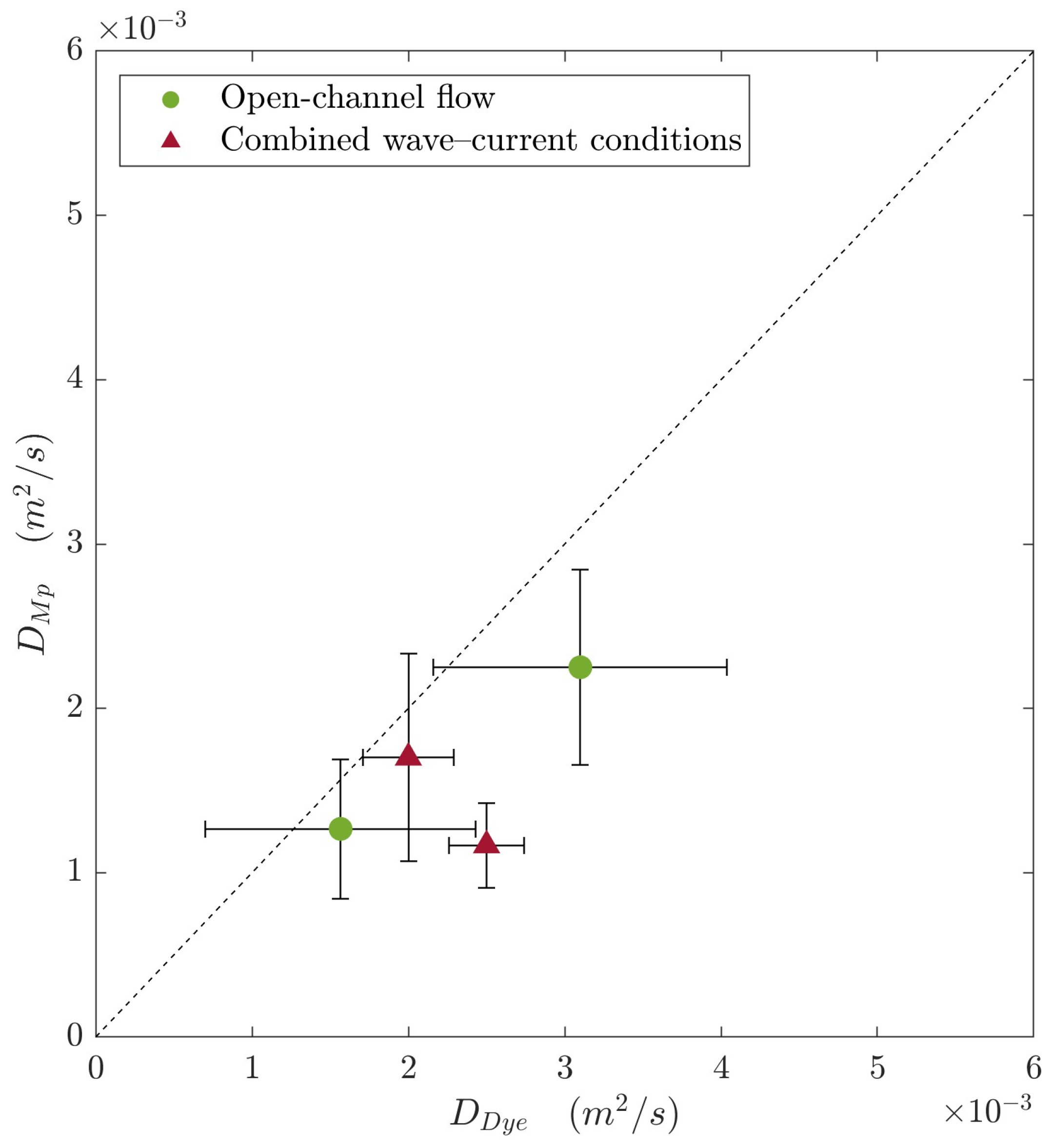
4.1. Longitudinal Dispersion

When the tracer cloud moved downstream along the flume, the concentration time series created by the cloud was measured by four fluorometers located in fixed positions along the flume. Figure 2 presents a typical concentration time series diagram, measured using a series of fluorometers along the flow. For all tested experimental conditions, it was observed that the concentration time series of the microplastic tracer consisted of more noise. This is attributed to the discrete nature of suspended microplastic particles compared to the solute dye. Consequently, the moving average was calculated for the tracer time series to reduce the noise of the raw data before carrying out further analysis. This was performed for both the dye and microplastics for consistency even though the raw data for dye have less noise.

The longitudinal dispersion coefficients were calculated based on the rate of change of variance of the tracer clouds travelling downstream along the flume using Equation (4). Since the measurements were collected at four stations, the rate of change of variance was calculated by plotting the best-fit line for all four stations. The calculated longitudinal dispersion coefficients are summarized in

Table 2. Longitudinal dispersion coefficients.

Flow Rate ($\mathit{Q}$) (L/s)	Hydrodynamic Condition	Input Wave Steepness (S) (%)	Longitudinal Dispersion Coefficients (D) (m2/s) × 10−2
				Solute	Microplastics
5	Unidirectional flow	N/A	Repeat 1	0.17	0.15
			Repeat 2	0.20	0.13
			Repeat 3	0.10	0.10
			Average	0.16	0.13
5	Wave–current combined	3.77%	Repeat 1	0.18	0.18
			Repeat 2	0.21	0.16
			Repeat 3	0.21	-
			Average	0.20	0.17
5	Wave–current combined	6.53%	Repeat 1	0.24	0.12
			Repeat 2	0.26	0.11
			Repeat 3	-	0.12
			Average	0.25	0.12
7	Unidirectional flow	N/A	Repeat 1	0.32	0.20
			Repeat 2	0.25	0.25
			Repeat 3	0.36	-
			Average	0.31	0.23

, and they are visualized in Figure 3.

According to the observations, the longitudinal dispersion coefficients calculated from the buoyant microplastics is almost comparable to the longitudinal dispersion calculated from the solute dye. This observation for slow open-channel flow compliments the previous findings on microplastic dispersion in open-channel flows [24], and the tested slow open-channel flow conditions here are on the lower end of the range for previously studied channel flow velocities. If observed closely, the dispersion coefficients calculated from microplastic tracer is slightly lower than that of the solute dye for both hydrodynamic conditions: slow open-channel flows and combined wave–current conditions. Since the variability between repeat tests is also high, more evidence is needed to obtain a solid conclusion on this observation.

Since the polyethylene particles have a specific density of 0.94, which is slightly less than water, the expectation is that the microplastics will float and gather towards the water surface without being dispersed along the flow, especially for the very slow open-channel flow configurations, as the flow is not strong enough to force advection on the particles. Therefore, it is important to observe that the buoyant polyethylene is dispersing in a rather comparable manner to a solute dye even in a slow pond or wetland setting. It was also expected that the oscillatory motion induced by the waves would prevent the microplastics from floating in the slow background current, making the dispersion coefficients of combined wave–current flow of microplastics more comparable to solute dye than in the scenarios with slow open-channel flows. From the limited experimental data, a significant enhancement due to the wave action was not noted.

This is important due to two main reasons. Firstly, polyethylene is one of the most common microplastic type found in the environment, and this observation can be useful in water treatment practices. Secondly, the dispersion of solute in ponds and wetlands is governed by hydrodynamic processes of water if the solute acts as a passive tracer, which does not alter the properties of the fluid. Knowing that the effects due to the buoyancy in microplastics in water are negligible allows using established hydrodynamic models to predict polyethylene dispersion in water without taking its material properties into account, which simplifies computational procedures.

The longitudinal dispersion of microplastic tracer is about half of that measured by the solute tracer for combined wave–current conditions with the higher wave steepness (6.53%). In the literature, the effect of oscillatory motion on microplastic dispersion has not yet been studied in detail, and the limited experimental data from this study suggest that the oscillatory wave motion might push the microplastics towards the top of the water column due to the slightly lower density of polyethylene microplastics, causing them to mix in the vertical direction and reducing their dispersion in the longitudinal direction. It is recommended to measure concentrations in several vertical locations across the water column in future studies to check this phenomenon.

One major limitation of these experimental findings is the limited length of the flume in which the tests were carried out. The testing domain was about 7.5 m, which is considerably smaller compared to the natural ponds and wetlands. It would be fascinating to test whether the polyethylene particles start to float due to their lower density when the pathway is long and when the flow velocity is slow. Experimenting with microplastics in the natural waterways will cause an environmental hazard, and therefore, further testing on slow flow velocities in longer laboratory flumes will be useful in drawing a concrete conclusion on this topic. For an example, because the motion of a microplastic particle in a marine environment is driven by physical forces—the weight, buoyancy, and drag [35]—a simple calculation shows that an average flow velocity of 0.01 m/s (a corresponding flow rate of 0.85 L/s) will require a testing domain of at least 14.3 m of length in order to showcase the effects due to the floatation of polyethylene particles for a water depth of 0.25 m at 25 °C, assuming the effect on the upward movement of polyethylene particles due to turbulence is minimal. Hence, these experimental findings should be carefully applied for average dispersion over longer stretches with still to very slow flow velocities such as wastewater treatment ponds and constructed wetlands. Also, these experimental findings will not be applicable straightaway when evaluating the streamwise dispersal properties of various other microplastic particle types with different specific densities.

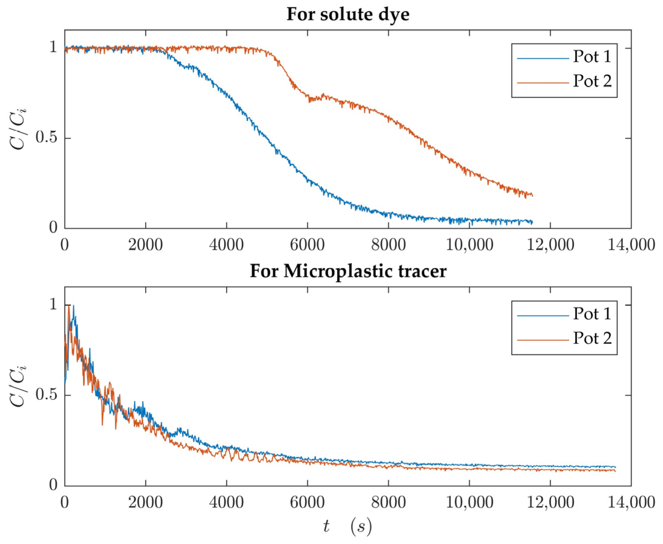
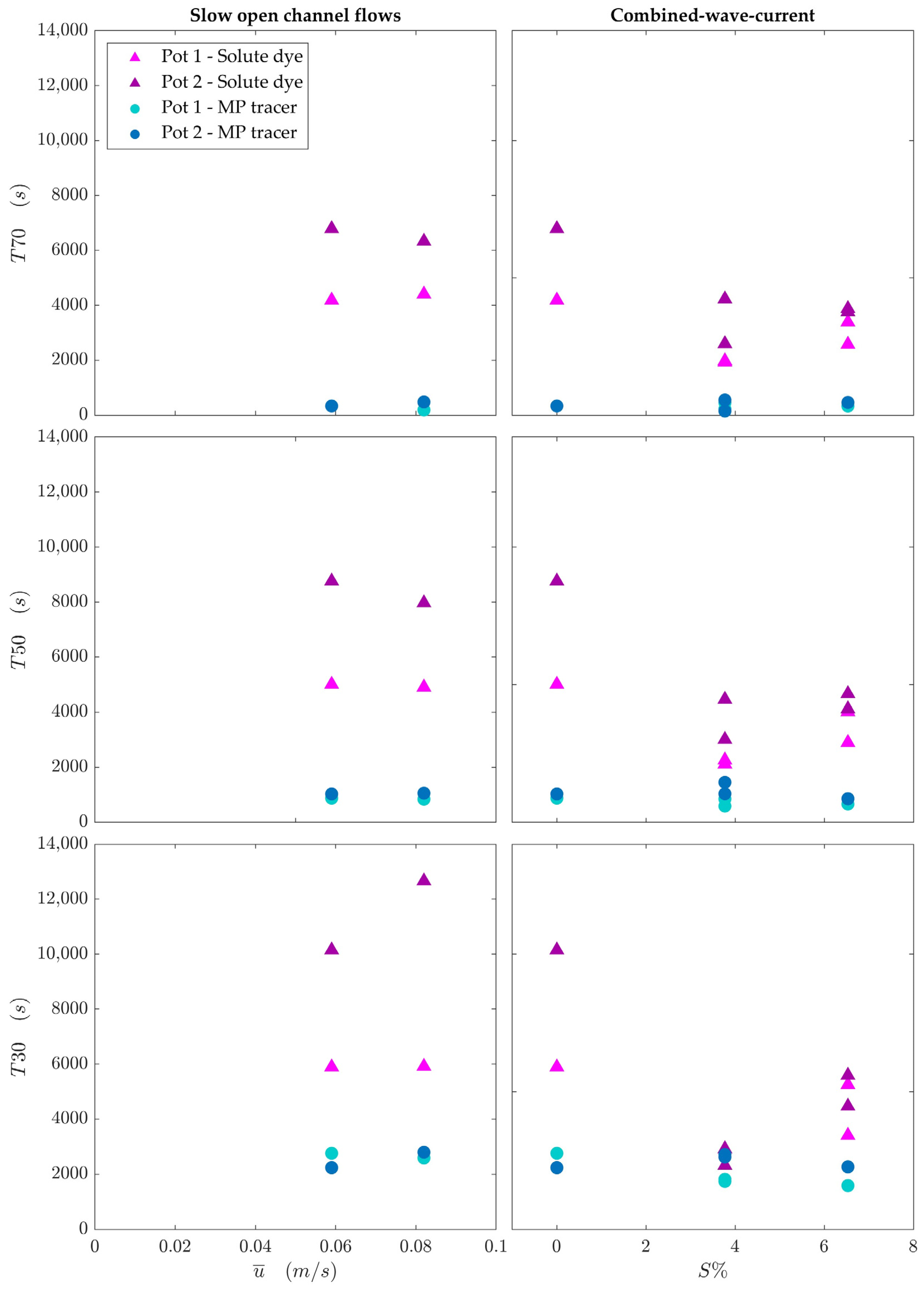
4.2. Mixing across the Hyporheic Zone

For the hyporheic exchange tests, the tracer concentrations inside the pots were at their highest in the beginning, and then, the concentrations decreased with time. Examples of the dimensionless concentration curves obtained using the solute dye and the microplastic tracer for slow open-channel flows and combined wave–current conditions are shown in Figure 4 and Figure 5. Similar to the longitudinal dispersion curves, the microplastic tracer concentration curves consist of more scatter.

The solute dye concentration remained constant in the beginning of the experiment before starting to drop, while the microplastic concentration started dropping at the beginning of the test. The time lag for the solute concentration’s decrease can be explained by the location of the fluorometer. The fluorometer was located 150 mm deep in the riverbed, and in the beginning of the experiment, the solute concentration was homogeneous throughout the pot. In the beginning of the test, the solute at the top started mixing with the upper part of the water column, and it took a significant time for this dilution process to reach the location of the fluorometer. Hence, the concentration curves for solute dye follow Fick’s second law.

When it comes to polyethylene microplastics, it is evident that the concentration started to decrease from the beginning. This can be explained by the low specific density of polyethylene, meaning that the polyethylene tracer particles started to float inside the pot, making the concentration decrease around the fluorometer located in the bottom of the pot. The microplastic tracer particles that floated in the pot could easily exit through the top eventually and enter the water flow above. The vertical transport of microplastic tracer through the porous sediment bed was also restrained by the trapping of microplastics around the glass spheres (replicating bed sediments); hence, the rate of change of microplastic tracer concentration decreased with time. While solute mixing across the hyporheic zone was governed by the diffusion process of solute dye inside the bed and the effects due to the hydrodynamics in the upper waterbody, the mixing of polyethylene microplastics across the hyporheic zone was governed by buoyancy and entrapping in addition to the aforementioned solute diffusion processes and the effects from the hydrodynamics above the bed.

To compare the different concentration curves with each other, the time taken to reach 70%, 50%, and 30% of the initial concentration inside the pots (T70, T50, and T30) was identified from the concentration time series, and the results are plotted in Figure 6. The diagrams on the left side of the matrix are for the slow open-channel flow conditions (without waves), and the diagrams on the right show waves with different magnitudes of steepness propagating on a background current of 0.059 m/s. In the same diagram, the T70, T50, and T30 values calculated for the current-only condition (without waves) are also plotted as a wave condition with zero wave steepness to demonstrate the effect due to the addition of waves. Two colour intensities are used for the two pots to differentiate the behaviour of the two pots.

The T70, T50, and T30 values calculated using the solute dye for pot 2 are always higher than that of pot 1. Pot 1, which was located closer to the inlet, tended to empty faster due to the increased turbulence caused by the inflow. When the T70, T50, and T30 values obtained using the microplastic tracer are considered, all these values are considerably smaller compared to those obtained using solute dye. This is attributed to the higher speed of the microplastic tracers than the solute dye when leaving the pots. Also, the T70, T50, and T30 values obtained using microplastic tracers for pot 1 and pot 2 are close to each other, and do not show any noticeable trend based on the location of the pot. This shows that the movement of microplastics is strongly dominated by buoyancy, and the effect due to inlet turbulence (in the upper waterbody) becomes negligible in controlling the fate of microplastic tracer. Polyethylene has a specific density close to 1, which makes it neutrally buoyant. Mixing across the hyporheic zone is a slow process, and due to the extended time during which the mixing takes place, the polyethylene had enough time to float, allowing the small difference in densities to govern the process. This observation will be useful when studying groundwater pollution, as this also suggests that fine microplastics with a specific density above 1 will move downwards.

According to Figure 6, the T50 values obtained from the repeat tests are slightly different from each other, denoting that averaged values from a higher number of repetitions are needed to obtain concrete conclusions. Therefore, for this study, efforts were made to provide a qualitative discussion instead of presenting empirical numerical relationships.

Experimental investigations on the diffusivity of neutrally buoyant microplastics across the hyporheic zone are extremely scarce. This study provides an insight into this topic, and further testing will expand the understanding on the behaviour of various microplastic particle types with different specific densities and shapes. Since the mixing of the microplastic tracer across the hyporheic zone was governed by buoyancy and gravity, equations based on Fickian diffusion were not applied for quantifying, as this also needs more experimental data for validations. Instead, a simple relationship between the T70, T50, and T30 values calculated based on the microplastic tracer and solute dye is presented in

Table 3. Comparison of T70, T50, and T30 values obtained for solute dye and microplastic tracers.

Flow Rate (Q) (L/s)	Scenario	Input Wave Steepness (S) (%)	$\frac{{\mathbf{T}70}_{\mathit{D}\mathit{y}\mathit{e}}}{{\mathbf{T}70}_{\mathbf{M}\mathbf{P}}}$	$\frac{{\mathbf{T}50}_{\mathit{D}\mathit{y}\mathit{e}}}{{\mathbf{T}50}_{\mathbf{M}\mathbf{P}}}$	$\frac{{\mathbf{T}30}_{\mathit{D}\mathit{y}\mathit{e}}}{{\mathbf{T}30}_{\mathbf{M}\mathbf{P}}}$
5	Open channel flow	N/A	16.48	7.23	3.21
5	Combined wave–current	3.77%	6.61	2.69	1.43
5	Combined wave–current	6.53%	15.83	10.27	4.77
7	Open channel flow	N/A	16.17	6.79	6.91

for the ease of recreating the concentration variations of the microplastic tracer for the given test conditions.

5. Conclusions

The diffusive behaviour of neutrally buoyant microplastic particles in a benthic environment (polyethylene, specific density: 0.94) was compared with solute using the limited experimental data based on streamwise dispersion and mixing across a hyporheic zone. When the streamwise dispersion properties on slow open-channel flows and combined wave–current conditions are considered, the behaviour of neutrally buoyant microplastics was comparable to solute dye for the tested range of flow and wave conditions. When the mixing across the hyporheic zone was studied, the longer timespans associated with the process allowed the slightly lower density of polyethylene to dominate, making the microplastics leave the pot faster than the solute. It was noticed that the solute mixing across the hyporheic zone was influenced by the hydrodynamics in the upper waterbody, while the movement of the microplastic tracer across the hyporheic zone was mainly dominated by the buoyancy. Longitudinal mixing studies on longer channels with low flow rates will further increase the understanding of the behaviour of neutrally buoyant microplastics during longer timespans.

References

1. Frias, J.; Nash, R. Microplastics: Finding a consensus on the definition. Mar. Pollut. Bull. 2018, 138, 145–147. [Google Scholar] [CrossRef] [PubMed]
2. Alimi, O.S.; Farner Budarz, J.; Hernandez, L.M.; Tufenkji, N. Microplastics and Nanoplastics in Aquatic Environments: Aggregation, Deposition, and Enhanced Contaminant Transport. Environ. Sci. Technol. 2018, 52, 1704–1724. [Google Scholar] [CrossRef] [PubMed]
3. Derraik, J.G.B. The pollution of the marine environment by plastic debris: A review. Mar. Pollut. Bull. 2002, 44, 842–852. [Google Scholar] [CrossRef] [PubMed]
4. Chang, M. Reducing microplastics from facial exfoliating cleansers in wastewater through treatment versus consumer product decisions. Mar. Pollut. Bull. 2015, 101, 330–333. [Google Scholar] [CrossRef]
5. Sharma, S.; Chatterjee, S. Microplastic pollution, a threat to marine ecosystem and human health: A short review. Environ. Sci. Pollut. Res. 2017, 24, 21530–21547. [Google Scholar] [CrossRef]
6. Hu, Y.; Gong, M.; Wang, J.; Bassi, A. Current research trends on microplastic pollution from wastewater systems: A critical review. Rev. Environ. Sci. Bio/Technol. 2019, 18, 207–230. [Google Scholar] [CrossRef]
7. Uurasjärvi, E.; Hartikainen, S.; Setälä, O.; Lehtiniemi, M.; Koistinen, A. Microplastic concentrations, size distribution, and polymer types in the surface waters of a northern European lake. Water Environ. Res. 2019, 92, 149–156. [Google Scholar] [CrossRef]
8. Coyle, R.; Hardiman, G.; Driscoll, K.O. Microplastics in the marine environment: A review of their sources, distribution processes, uptake and exchange in ecosystems. Case Stud. Chem. Environ. Eng. 2020, 2, 100010. [Google Scholar] [CrossRef]
9. Eriksen, M.; Lebreton, L.C.M.; Carson, H.S.; Thiel, M.; Moore, C.J.; Borerro, J.C.; Galgani, F.; Ryan, P.G.; Reisser, J. Plastic Pollution in the World’s Oceans: More than 5 Trillion Plastic Pieces Weighing over 250,000 Tons Afloat at Sea. PLoS ONE 2014, 9, e111913. [Google Scholar] [CrossRef]
10. Woodall, L.C.; Sanchez-Vidal, A.; Canals, M.; Paterson, G.L.J.; Coppock, R.; Sleight, V.; Calafat, A.; Rogers, A.D.; Narayanaswamy, B.E.; Thompson, R.C. The deep sea is a major sink for microplastic debris. R. Soc. Open Sci. 2014, 1, 140317. [Google Scholar] [CrossRef]
11. Browne, M.A.; Galloway, T.S.; Thompson, R.C. Spatial Patterns of Plastic Debris along Estuarine Shorelines. Environ. Sci. Technol. 2010, 44, 3404–3409. [Google Scholar] [CrossRef] [PubMed]
12. Jamieson, A.J.; Brooks, L.S.R.; Reid, W.D.K.; Piertney, S.B.; Narayanaswamy, B.E.; Linley, T.D. Microplastics and synthetic particles ingested by deep-sea amphipods in six of the deepest marine ecosystems on Earth. R. Soc. Open Sci. 2019, 6, 180667. [Google Scholar] [CrossRef] [PubMed]
13. Mato, Y.; Isobe, T.; Takada, H.; Kanehiro, H.; Ohtake, C.; Kaminuma, T. Plastic Resin Pellets as a Transport Medium for Toxic Chemicals in the Marine Environment. Environ. Sci. Technol. 2000, 35, 318–324. [Google Scholar] [CrossRef] [PubMed]
14. Taylor, M.L.; Gwinnett, C.; Robinson, L.F.; Woodall, L.C. Plastic microfibre ingestion by deep-sea organisms. Sci. Rep. 2016, 6, 33997. [Google Scholar] [CrossRef]
15. Wu, H.; Hou, J.; Wang, X. A review of microplastic pollution in aquaculture: Sources, effects, removal strategies and prospects. Ecotoxicol. Environ. Saf. 2023, 252, 114567. [Google Scholar] [CrossRef]
16. Jain, R.; Gaur, A.; Suravajhala, R.; Chauhan, U.; Pant, M.; Tripathi, V.; Pant, G. Microplastic pollution: Understanding microbial degradation and strategies for pollutant reduction. Sci. Total. Environ. 2023, 905, 167098. [Google Scholar] [CrossRef]
17. James, I. Modelling pollution dispersion, the ecosystem and water quality in coastal waters: A review. Environ. Model. Softw. 2002, 17, 363–385. [Google Scholar] [CrossRef]
18. Chen, Y.; Zeng, L. A holistic model for microplastic dispersion in a free-surface wetland flow. J. Clean. Prod. 2024, 449. [Google Scholar] [CrossRef]
19. Rowlands, E.; Galloway, T.; Cole, M.; Peck, V.L.; Posacka, A.; Thorpe, S.; Manno, C. Vertical flux of microplastic, a case study in the Southern Ocean, South Georgia. Mar. Pollut. Bull. 2023, 193, 115117. [Google Scholar] [CrossRef]
20. Wagner, M.; Lambert, S. (Eds.) Freshwater Microplastics; Springer Nature: Dordrecht, The Netherlands, 2018; Volume 58. [Google Scholar] [CrossRef]
21. Okamura, T. Polyethylene (PE.; Low Density and High Density). In Encyclopedia of Polymeric Nanomaterials; Springer: Berlin/Heidelberg, Germany, 2015; pp. 1826–1829. [Google Scholar] [CrossRef]
22. Lavers, J.L.; Oppel, S.; Bond, A.L. Factors influencing the detection of beach plastic debris. Mar. Environ. Res. 2016, 119, 245–251. [Google Scholar] [CrossRef]
23. Erni-Cassola, G.; Gibson, M.I.; Thompson, R.C.; Christie-Oleza, J.A. Lost, but Found with Nile Red: A Novel Method for Detecting and Quantifying Small Microplastics (1 mm to 20 μm) in Environmental Samples. Environ. Sci. Technol. 2017, 51, 13641–13648. [Google Scholar] [CrossRef] [PubMed]
24. Cook, S.; Chan, H.-L.; Abolfathi, S.; Bending, G.D.; Schäfer, H.; Pearson, J.M. Longitudinal dispersion of microplastics in aquatic flows using fluorometric techniques. Water Res. 2020, 170, 115337. [Google Scholar] [CrossRef] [PubMed]
25. Filippi, M.; Hanlon, R.; Rypina, I.I.; Hodges, B.A.; Peacock, T.; Schmale, D.G. Tracking a Surrogate Hazardous Agent (Rhodamine Dye) in a Coastal Ocean Environment Using In Situ Measurements and Concentration Estimates Derived from Drone Images. Remote. Sens. 2021, 13, 4415. [Google Scholar] [CrossRef]
26. Stride, B.; Stride, B.; Abolfathi, S.; Abolfathi, S.; Odara, M.G.N.; Odara, M.G.N.; Bending, G.D.; Bending, G.D.; Pearson, J.; Pearson, J. Modeling Microplastic and Solute Transport in Vegetated Flows. Water Resour. Res. 2023, 59. [Google Scholar] [CrossRef]
27. Stride, B.; Abolfathi, S.; Bending, G.D.; Pearson, J. Quantifying microplastic dispersion due to density effects. J. Hazard. Mater. 2024, 466, 133440. [Google Scholar] [CrossRef]
28. Fick, A.V. On liquid diffusion. Lond. Edinb. Dublin Philos. Mag. J. Sci. 1855, 10, 30–39. [Google Scholar] [CrossRef]
29. Elder, J.W. The dispersion of marked fluid in turbulent shear flow. J. Fluid Mech. 1959, 5, 544–560. [Google Scholar] [CrossRef]
30. Fischer, H.B.; List, E.J.; Koh, R.C.Y.; Imberger, J.; Brooks, N.H. Chapter 2: Fickian Diffusion. In Mixing in Inland and Coastal Waters, 1st ed.; Academic Press: Amsterdam, The Netherlands, 1979; Chapter 2; pp. 30–50. [Google Scholar]
31. Chandler, I.D.; Guymer, I.; Pearson, J.M.; van Egmond, R. Vertical variation of mixing within porous sediment beds below turbulent flows. Water Resour. Res. 2016, 52, 3493–3509. [Google Scholar] [CrossRef]
32. Stern, D.A.; Khanbilvardi, R.; Alair, J.C.; Richardson, W. Description of flow through a natural wetland using dye tracer tests. Ecol. Eng. 2001, 18, 173–184. [Google Scholar] [CrossRef]
33. Law, K.L. Plastics in the Marine Environment. Annu. Rev. Mar. Sci. 2017, 9, 205–229. [Google Scholar] [CrossRef]
34. Clark, L.K.; DiBenedetto, M.H.; Ouellette, N.T.; Koseff, J.R. Dispersion of finite-size, non-spherical particles by waves and currents. J. Fluid Mech. 2022, 954, A3. [Google Scholar] [CrossRef]
35. Chubarenko, I.; Bagaev, A.; Zobkov, M.; Esiukova, E. On some physical and dynamical properties of microplastic particles in marine environment. Mar. Pollut. Bull. 2016, 108, 105–112. [Google Scholar] [CrossRef]
Figure 1. Experimental setup. The numbered elements are as follows: (1) foam body to absorb the reversed waves created by the movement of the wave paddle; (2) piston wave paddle; (3) Cyclops-7 fluorometers for measuring the concentrations in the water column; (4) adjustable outlet weir with energy dissipating batons glued on top; (5) pots for measuring the mixing across the hyporheic zone; (6) rubber tube that goes through a peristaltic pump to a container filled with solute/microplastic tracers forming the injection system; (7) centrifugal pump; (8) water storage tank. The following numbers explain the individual elements that make up the pots: (9) stainless-steel mesh that keeps the glass beads in place; (10) arrangement used for connecting the pots to the bottom of the flume; (11) 5 mm glass spheres; (12) cylindrical pot made out of a PVC tube; (13) non-return valve that prevents the tracers from leaving the pots; (14) inlet tube that feeds the microplastic/solute tracers into the pots; (15) stainless-steel cylindrical mesh that creates a clear region around the fluorometer; (16) Cyclops-7 fluorometer that measures the solute/microplastic tracer concentration inside the pot.
Microplastics 03 00032 g001
Figure 2. Examples of typical concentration time series measured along the flow. The data correspond to an open-channel flow with a flow rate of 7 L/s.
Microplastics 03 00032 g002
Figure 3. The longitudinal dispersion coefficient calculated from the microplastic tracer compared to that calculated from solute dye. The error bars denote 90% confidence interval.
Microplastics 03 00032 g003
Figure 4. The typical tracer concentration variation inside the pots for slow open-channel flows. The presented data correspond to an open-channel flow condition with an average background current velocity 0.059 m/s.
Microplastics 03 00032 g004
Figure 5. The typical tracer concentration variation inside the pots for combined wave–current conditions. The presented data correspond to a wave (with steepness 3.77%) propagating on a background current with an average velocity of 0.059 m/s.
Microplastics 03 00032 g005
Figure 6. T70, T50, and T30 values calculated using the solute dye and the microplastic tracer for slow open-channel flow conditions and combined wave–current conditions.
Microplastics 03 00032 g006