Comparison of Univariate and Multivariate Applications of GBLUP and Artificial Neural Network for Genomic Prediction of Growth and Carcass Traits in the Brangus Heifer Population

Simple Summary

The aim of this study was to compare the predictive performances of genomic best linear unbiased prediction models and 1-10-neuron artificial neural network models with the learning algorithms of Bayesian Regularization, Levenberg–Marquardt and Scaled Conjugate Gradient and transfer function combinations of tangent sigmoid–linear and linear–linear in the hidden-output layers based on the input from the genomic relationship matrix in univariate and multivariate analyses of growth and carcass traits from Brangus heifers. Pearson’s correlation coefficients calculated between observed and predicted phenotypes for traits were used to determine the predictive performances of univariate and multivariate genomic best linear unbiased prediction and 1-10-neuron artificial neural network models with learning algorithms and transfer function combinations. The results indicated that genomic best linear unbiased prediction models and artificial neural network models in the univariate analysis of growth and carcass traits resulted in better predictive performances than those of models in the multivariate analysis. In the univariate analysis, models with the Bayesian Regularization learning algorithm yielded higher predictive performances than models with Levenberg–Marquardt or Scaled Conjugate Gradient backpropagation learning algorithms and genomic best linear unbiased prediction models. The predictive performances of models with the tangent sigmoid–linear transfer function combination were also better than those with the linear–linear transfer function combination in the univariate analysis. The complex architectures of artificial neural network models and genetic relationship among growth and carcass traits could cause lower and poor predictive performances in multivariate analysis.

Abstract

Data for growth (birth, weaning and yearling weights) and carcass (longissimus muscle area, intramuscular fat percentage and depth of rib fat) traits and 50K SNP marker data to calculate the genomic relationship matrix were collected from 738 Brangus heifers. Univariate and multivariate genomic best linear unbiased prediction models based on the genomic relationship matrix and univariate and multivariate artificial neural networks models with 1 to 10 neurons, as well as the learning algorithms of Bayesian Regularization, Levenberg–Marquardt and Scaled Conjugate Gradient and transfer function combinations of tangent sigmoid–linear and linear–linear in the hidden-output layers, including the inputs from genomic relationship matrix, were created and applied for the analysis of growth and carcass data. Pearson’s correlation coefficients were used to evaluate the predictive performances of univariate and multivariate genomic best linear unbiased prediction and artificial neural networks models. The overall predictive abilities of genomic best linear unbiased prediction and artificial neural network models were low in the univariate and multivariate analysis. However, the predictive performances of models in the univariate analysis were significantly higher than those from models in the multivariate analysis. In the univariate analysis, models with Bayesian Regularization and the tangent sigmoid–linear or linear–linear transfer function combination yielded higher predictive performances than models with learning algorithms and genomic best linear unbiased prediction models. In addition, predictive performances of models with tangent sigmoid–linear transfer functions were better than those with linear–linear transfer functions in the univariate analysis.

1. Introduction

There is growing interest in improving economically important traits in beef cattle breeding programs to increase the profitability of beef cattle production systems. Among several economically important traits, growth-related traits including birth weight (BW), weaning weight (WW) and yearling weight (YW) are traditionally considered selection criteria in beef cattle breeding. Carcass traits including the depth of rib fat (FAT), intramuscular fat percentage (IMF) and longissimus muscle area (LMA) have also gained importance in the selection programs of beef cattle breeding in order to fulfill the market quality standards and consumer perceptions of meat [1,2,3]. Genomic selection has been applicable for economically important traits since the availability of high-density single-nucleotide polymorphism (SNP) markers [1,2,3,4] and the statistical methods for genomic prediction [1,5,6]. Many statistical methods (such as GBLUP, BayesA, BayesB, BayesC and Bayesian Lasso) for genomic prediction work based on capturing the association between SNP marker genotypes and phenotypes of a trait and then, by fitting the association, learn how SNP marker genotypes map to the quantity to be predicted.

Genetic gains in many plant and animal breeding programs were achieved using pedigree-based best linear unbiased prediction (BLUP) methods. The genomic BLUP (GBLUP) method was developed by replacing pedigree-based additive genetic relationships with genomic relationships (observed similarity at the genomic level) estimated from SNP markers. Hence, the dimensions of genetic effects in the univariate and multivariate mixed linear models are reduced by the number of individuals in the population, resulting in a computationally more efficient statistical model. The accuracy of the genomic estimated breeding value (GEBV) can be calculated in the same way as in pedigree-based BLUP.

In the last decade, artificial neural networks (ANNs) have been considered different learning methods for genomic prediction. The development and use of ANNs for artificial intelligence was inspired by the operations of nerve cells (known neurons) in the human brain. The ANN is a statistical modeling of the human brain functions and represents a new generation of information processing systems [7]. The learning ability of ANNs without using any prior assumption and sophisticated statistical models for linear and non-linear relationships in information processing systems is a very attractive feature. ANN methods are nonparametric models providing tremendous flexibility to adapt to complicated associations between data and output. Their particular strength is the ability to adapt to hidden patterns of an unknown structure that therefore could not have been incorporated into a parametric model at the beginning [8]. Therefore, ANN statistical models have been used to predict the genomic values of individuals for complex traits within the last decade because complex quantitative traits, such as growth and production traits in animal and plant breeding, are controlled by a network of numerous genes [9].

This study aimed to compare the predictive performances of univariate and multivariate GBLUP and 1-10-neuron ANN models with learning algorithms (Levenberg–Marquardt (LM), Bayesian Regularization (BR) and Scaled Conjugate Gradient (SCG)) and transfer functions (tangent sigmoid and linear) using the input from the G genomic relationship matrix in analyses of growth and carcass traits.

2. Materials and Methods

2.1. Phenotypes, SNP Markers and Genomic Relationship Matrix

Data for growth (birth weight (BW), weaning weight (WW) and yearling weight (YW)) and carcass (depth of rib fat (FAT), intramuscular fat percentage (IMF) and longissimus muscle area (LMA)) traits were obtained from 738 Brangus heifers raised in Camp Cooley Ranch, east-central Texas, and the Chihuahuan Desert Rangeland Research Center and Campus Farm, New Mexico State University, in the spring or fall calving season of the 2005 through 2007 birth years [10,11,12]. Dam age and weaning and yearling contemporary groups created based on year of birth (2005 to 2007) and season of calving (spring or autumn) were considered as potential fixed factors affecting the growth (BW, WW and YW) and carcass (FAT, IMF and LMA) traits. Therefore, growth and carcass traits were adjusted for these fixed factors to make fair and objective comparisons between univariate and multivariate GBLUP and 1-10-neuron ANN models.

SNP marker genotypes (AA, AB, BB) of 738 Brangus heifers were obtained using BovineSNP50 Infinium BeadChips (Illumina, San Diego, CA, USA) for 53,692 SNP markers [2]. Three filters were applied for the quality control of SNP markers using the snpReady package in the R program [13]: heifers were retained if (a) the genotype call rate was greater than 95% and (b) the number of missing observations was less than 50%, and (c) SNP markers with a minor allele frequency (MAF) greater than 10% were retained. Then, the imputation of missing SNP marker genotypes resulted in 738 animals with 35,351 SNP markers.

The genomic relationship matrix ($\mathit{G}$) [14,15] was calculated using 35,351 SNP markers as follows:

$$\mathit{G}={\displaystyle \frac{(\mathit{M}-\mathit{P})({\mathit{M}-\mathit{P})}^{\prime }}{2{\sum }_{i=1}^k{p}_i(1-p_i)}}$$

where ${\mathit{M}}_{(n \times k)}$ is the matrix of the coded (0 for AA; 1 for AB; 2 for BB) $k=\mathrm{35,351}$ SNP marker genotypes for the $n=738$ animals; ${\mathit{P}}_{(n \times k)}$ is the matrix for allele frequencies of the SNP markers multiplied by 2, $p_i$ is the allele frequency of ith SNP marker, and the sum is over all loci.

2.2. Genomic Best Linear Unbiased Prediction

Genomic best linear unbiased prediction (GBLUP), introduced by Habier et al. [14] and vanRaden [15], is a method using genomic information through the genomic relationship matrix ($\mathit{G}$). Univariate and multivariate mixed linear models for genome-base-estimated breeding values were fitted for the growth (BW, WW and YW) and carcass (FAT, IMF and LMA) traits:

Univariate model:

$${\mathit{y}}_i={\mathit{X}}_i{\mu }_i+{\mathit{Z}}_i{\mathit{g}}_i+{\mathit{e}}_i i=\{BW, WW, YW,FAT, IMF, LMA\}$$

where ${\mathit{y}}_i$ is the vector of adjusted phenotypes for the ith growth (BW, WW and YW) or carcass (FAT, IMF and LMA) trait, ${\mathit{X}}_i$ and ${\mathit{Z}}_i$ are the design matrices for the fixed (overall mean) and random additive genetic effects, ${\mu }_i$ is the overall mean, ${\mathit{g}}_i$ is the vector of random additive genetic effects for the ith growth (BW, WW and YW) or carcass (FAT, IMF and LMA) trait, which is assumed to be distributed as multivariate normal, with null mean vector and (co)variance matrix $\mathit{G}{\sigma }_{gi}^2$, where $\mathit{G}$ is the genomic relationship matrix and ${\sigma }_{gi}^2$ is the additive genetic variance. ${\mathit{e}}_i$ is the vector of random residual effects for the ith growth (BW, WW and YW) or carcass (FAT, IMF and LMA) trait, which is assumed to be distributed as multivariate normal, with null mean vector and (co)variance matrix $\mathit{I}{\sigma }_{ei}^2$, where $\mathit{I}$ is the identity matrix and ${\sigma }_{ei}^2$ is the residual variance.

Multivariate model:

$$\left[\begin{array}{c}{\mathit{y}}_{BW}\\ ⋮\\ {\mathit{y}}_{LMA}\end{array}\right]=\left[\begin{array}{ccc}{\mathit{X}}_{BW}& \cdots & 0\\ ⋮& \ddots & ⋮\\ 0& \cdots & {\mathit{X}}_{LMA}\end{array}\right]\left[\begin{array}{c}{\mu }_{BW}\\ ⋮\\ {\mu }_{LMA}\end{array}\right]+\left[\begin{array}{ccc}{\mathit{Z}}_{BW}& \cdots & 0\\ ⋮& \ddots & ⋮\\ 0& \cdots & {\mathit{Z}}_{LMA}\end{array}\right]\left[\begin{array}{c}{\mathit{g}}_{BW}\\ ⋮\\ {\mathit{g}}_{LMA}\end{array}\right]+\left[\begin{array}{c}{\mathit{e}}_{BW}\\ ⋮\\ {\mathit{e}}_{LMA}\end{array}\right]$$

${\mathit{y}}_{BW}\cdots {\mathit{y}}_{LMA}$ are the vectors of adjusted phenotypes for growth (BW, WW and YW) and carcass (FAT, IMF and LMA) traits, ${\mathit{X}}_{BW}\cdots {\mathit{X}}_{LMA}$ are the design matrices for the fixed (overall mean) effects, ${\mathit{Z}}_{BW}\cdots {\mathit{Z}}_{LMA}$ are the design matrices for the random (additive genetic) effects, ${\mu }_{BW}\cdots {\mu }_{LMA}$ are the vectors of fixed effects (means), ${\mathit{g}}_{BW}\cdots {\mathit{g}}_{LMA}$ are the vectors of random additive genetic effects assumed to be distributed as multivariate normal, with null mean vector and (co)variance matrix $\mathit{G}⨂\mathit{\Sigma }$, where $\mathit{\Sigma }$ is the additive genetic (co)variance matrix and $⨂$ denotes the Kronecker product. ${\mathit{e}}_{BW}\cdots {\mathit{e}}_{LMA}$ are the vectors of random residuals assumed to be distributed as multivariate normal, with null mean vector and (co)variance matrix $\mathit{I}⨂\mathit{R}$, where $\mathit{R}$ is the residual (co)variance matrix.

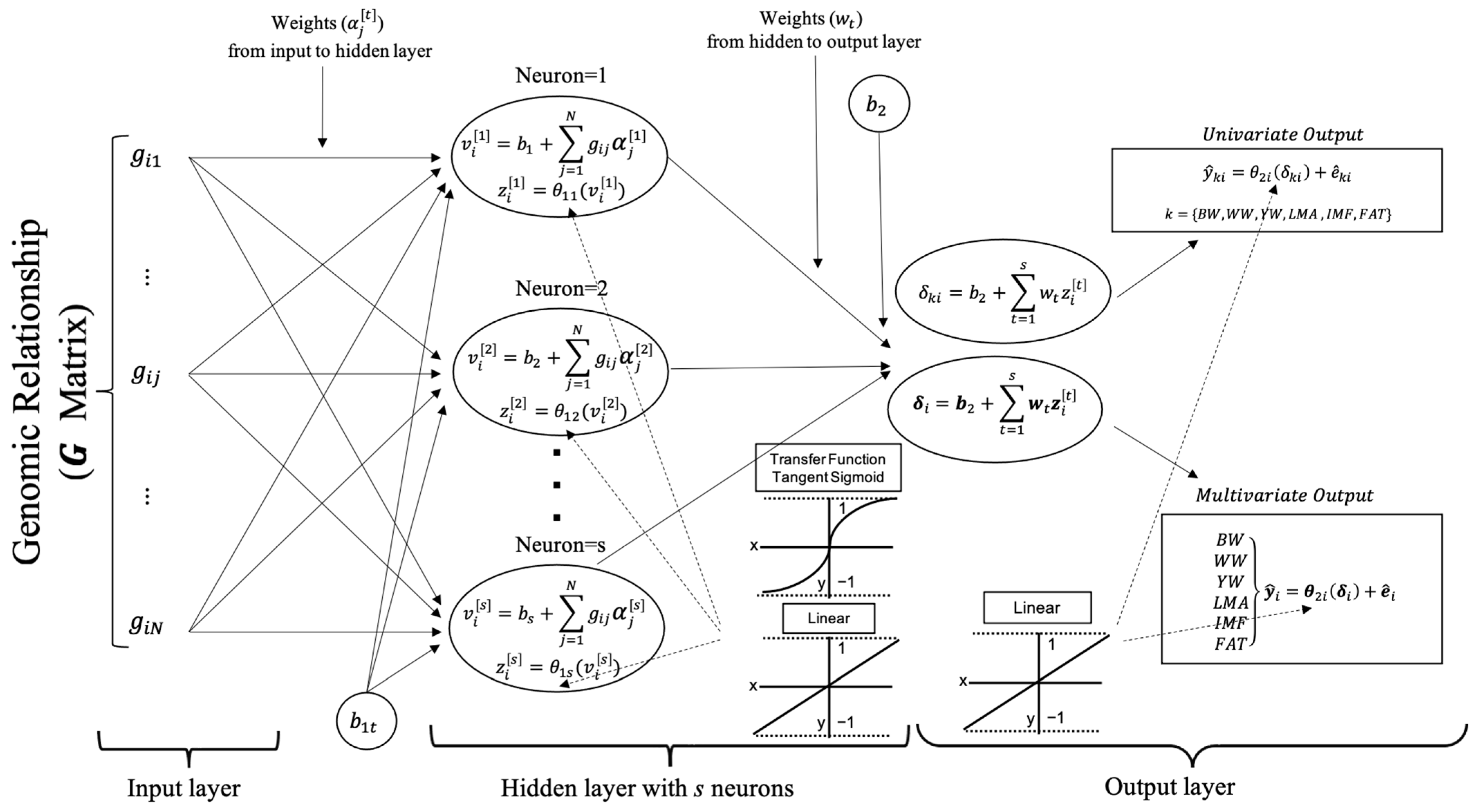
2.3. Artificial Neural Networks

Artificial neural networks (ANNs) are a type of non-linear model frequently used to predict genomic breeding values for genomic selection in the last decade. ANN models are computer algorithms, and their working principles are inspired by the function of the human brain and nervous system. The neurons of the human brain and their connections with each other establish the relationship among neurons as data processing units connected via adjustable weights (${\alpha }_j$) in the ANN. The ANN consists of an input layer, hidden layer(s) and an output layer. The interconnected neurons are arranged based on their functions in layers.

The Multi-Layer Perceptron Artificial Neural Network (MLPANN) includes many interconnected neurons that are grouped into an input layer, an intermediate or hidden layer and an output layer. The graphical representation of the MLPANN used for this study is given in Figure 1. As seen in Figure 1, genomic relationships ($g_{ij}$) between animals are independent variables and represent the input neurons in the input layer of the MLPANN model. Also, the growth (BW, WW and YW) and carcass (FAT, IMF and LMA) traits are dependent variables and represent the output neurons in the output layer of the MLPANN model.

The training process in the MLPANN focuses on increasing the estimation accuracy between predicted (output) values ($\widehat{\mathit{y}}$) and observed (actual) phenotypic values ($\mathit{y}$) using different numbers of neurons, learning algorithms and transfer functions in the hidden layer and producing univariate or multivariate outputs in the output layer.

2.3.1. Number of Neurons in Hidden Layer

The number of neurons ($s$) in hidden layers has a significant effect on the performance of the MLPANN model. The use of too few (one or two) neurons would not be enough to establish the unknown relationship between inputs and outputs in the MLPANN model; however, the use of too many neurons in the training process would cause an increase in complexity and execution time of the MLPANN model. From the literature, it was found that a single hidden layer was sufficient for an MLPANN model to approximate any complex non-linear function [16,17]; neurons between 1 and 10 ($t=1, 2,\dots , s=10$) were used in the MLPANN model (Figure 1).

2.3.2. Learning Algorithm in Hidden Layer

Learning in the ANN for genomic prediction is a training process that occurs by comparing the ANN predicted (output) value (${\widehat{y}}_i$) with the adjusted (actual) phenotypic value ($y_i$) and calculating the prediction error (${\widehat{e}}_i=y_i-{\widehat{y}}_i$) in the training data set. The backpropagation of prediction errors and the adjustment of connection weights are iteratively carried out by the learning algorithm [18], which attempts to reduce the global error by adjusting the weights and biases in the ANN procedure. Although many learning algorithms are indicated in the literature for the ANN procedure [19,20,21], it is difficult to determine the efficient one for genomic selection. Therefore, Bayesian Regularization (BR), Levenberg–Marquardt (LM) and Scaled Conjugate Gradient (SCG) backpropagation learning algorithms in this study were used to determine the faster learning and the better estimating ANN algorithm in the analysis of growth (BW, WW and YW) and carcass traits (FAT, IMF and LMA).

2.3.3. Transfer Functions in Hidden Layer

Transfer (activation) functions are used to calculate the outputs in the hidden and output layers during the training process in the MLPANN model. In this study, tangent sigmoid and linear transfer functions in the hidden layer were applied to calculate the outputs based on the association between inputs and outputs from the hidden layers in the MLPANN model (Figure 1). The tangent sigmoid and linear transfer functions are given in Figure 2:

• The tangent sigmoid transfer function $f\left(x\right)={\displaystyle \frac{2}{1+e^{-2x}}}-1$ produces the scaled output over the −1 to +1 closed range, which is obtained for $-\infty$ and $+\infty$, respectively [22,23]. Because there is a non-linear association between inputs and outputs, the TanSig function is widely used to determine these characteristics of the MLPANN model.
• Linear transfer function $f\left(x\right)=x$ produces an output in the range of $-\infty$ to $+\infty$ [24,25]. The association between inputs and outputs in the MLPANN models could not be non-linear and is determined by the purelin transfer function, which can be an acceptable representation of the input/output behavior in the MLPANN models.

As presented in Figure 2, the input layer in the MLPANN model distributes the genomic relationship values ($g_{ij}$) as an input signal to the neurons in the hidden layer. In the hidden layer, genomic relationship values $g_{ij}$ are combined with a vector of weights ${\alpha }^{\left[t\right]}=\left\{{\alpha }_{1j}^t\right\}$, plus a bias ($b_t$), at the hidden neuron $t$ ($t=1, 2,\dots , s=10$) in order to develop the score ${\nu }_i^{\left[t\right]}=(b_t+{\sum }_{j=1}^N{g}_{ij}{\alpha }_{1j}^{\left[t\right]})$ for animal $i$. Then, the resultant score ${\nu }_i^{\left[t\right]}=(b_t+{\sum }_{j=1}^N{g}_{ij}{\alpha }_{1j}^{\left[t\right]})$ is transformed using linear or tangent sigmoid activation functions to produce the output $z_i^{\left[t\right]}={\theta }_t({\nu }_i^{\left[t\right]})$ of hidden neuron $t$ for animal $i$ for the growth (BW, WW and YW) and carcass traits (FAT, IMF and LMA).

2.3.4. Univariate or Multivariate Outputs in Output Layer

The MLPANN model is applied for univariate (single-trait) analysis or multivariate (multiple-trait) analyses, and the univariate or multivariate outputs of neurons in the output layer were calculated using a transfer function (Figure 1 and Figure 2). The predictive performance of the MLPANN model can be affected by the univariate or multivariate structure of the output layer; therefore, in this study, the following applies:

• The univariate output of neurons in the output layer for the growth (BW, WW and YW) and carcass (FAT, IMF and LMA) traits is as follows:

  $${\widehat{y}}_{ki}={\theta }_{2i}\left({\delta }_{ki}\right)+{\widehat{e}}_{ki}$$

  where ${\delta }_{ki}=b_2+{\sum }_{t=1}^s{w}_t{z}_i^{\left[t\right]}$ and $k=\{BW,WW,YW,FAT,IMF,LMA\}$,
• The multivariate outputs of neurons in the output layer for the growth (BW, WW and YW) and carcass (FAT, IMF and LMA) traits are as follows:

  $$\left.\begin{array}{c}BW\\ WW\\ YW\\ FAT\\ IMF\\ LMA\end{array}\right\}{\widehat{\mathit{y}}}_i={\mathit{\theta }}_{2i}\left({\mathit{\delta }}_i\right)+{\widehat{\mathit{e}}}_i$$

  where ${\delta }_i=b_2+{\sum }_{t=1}^s{w}_t{z}_i^{\left[t\right]}$ was calculated using only the purelin ${\theta }_{2i}\left(.\right)$ transfer function (Figure 1 and Figure 2).

2.4. Cross-Validation and Predictive Performance of Artificial Neural Networks

Habier et al. [14] studied the effect of genomic relationships between animals in the training and validation data sets and showed that the accuracy of the GEBV of animals in the validation data set increases when the genomic relationship between animals in the validation data set and animals in the training data set increases. Saatchi et al. [26] also indicated that minimizing the genomic relationships between animals in the training and validation data sets, respectively, using a k-means clustering approach resulted in the accuracies of the GEBV of animals in the validation data set being less affected by their genomic relationships. Therefore, in this study, 10-fold cross-validation data sets were created from the genotyped animals using a k-means clustering approach based on the pedigree-based additive relationships [27]. GeneticsPed [28] and factoextra [29] packages in the R program were used to construct the pedigree-based numerator relationship ($\mathit{A}$) matrix and 10-fold cross-validation data sets based on the k-means clustering approach.

The training and validation processes in the cross-validation approach were carried out by taking nine cross-validation data sets from the 10-fold cross-validation data sets to train the univariate and multivariate GBLUP and ANN models and using the remaining cross-validation data set to predict the phenotypic values of animals from the omitted validation set. The predictive performance of the univariate and multivariate GBLUP and ANN models for growth (BW, WW and YW) and carcass (FAT, IMF and LMA) traits was evaluated by pooling the estimates of Pearson’s correlation coefficient ($r_{y_k,{\widehat{y}}_k}$) between the adjusted ($y_k$) and predicted phenotypic (${\widehat{y}}_k$) values from the 10-fold cross-validation data sets.

$$r_{y_k,{\widehat{y}}_k}={\displaystyle \frac{S_{y_k,{\widehat{y}}_k}}{\sqrt{S_{y_k}^2{S}_{{\widehat{y}}_k}^2}}}$$

where $S_{y_k,{\widehat{y}}_k}$ is the covariance between the adjusted ($y_k$) and predicted phenotypic (${\widehat{y}}_k$) values, and $S_{y_k}^2$ and $S_{{\widehat{y}}_k}^2$ are the variances for the adjusted ($y_k$) and predicted phenotypic (${\widehat{y}}_k$) values for trait $k$, respectively.

2.5. Analyses of Univariate and Multivariate GBLUP and MLPANN Models

The BGLR package (https://cran.r-project.org/web/packages/BGLR/index.html (ac-cessed on 13 February 2025)) in the R program [6] was used to estimate additive genetic effects ($\mathit{g}$) from univariate and multivariate GBLUP models.

The MATLAB Neural Network Toolbox Version 4.0 [30] was used to fit the MLPANN model in Figure 1. The applications of BR, LM and SCG learning algorithms were carried out utilizing the functions of trainlm(.), trainbr(.) and trainscg(.) in the MATLAB Neural Network Toolbox. The tangent sigmoid and linear transfer functions (Figure 2) for each learning (BR, LM and SCG) algorithm were applied using tansig(.) and purelin(.) functions in the MATLAB Neural Network Toolbox, respectively.

In this study, learning (BR, LM and SCG) algorithms were trained independently using 10 cross-validation data sets in order to establish good predictive ability and prevent overtraining in the training process of the MLPANN. During the training procedure, when weight parameter values at a current iteration did not change in the successive iteration, the training process stopped, and it was assumed that the convergence criteria of 1.0 × 10⁻⁶ was attained.

3. Results and Discussion

3.1. Comparison of Predictive Abilities of Univariate and Multivariate GBLUP and MLPANN Models

The genomic relationship estimated from SNP markers indicates realized genetic relatedness among animals [14,15], and the genomic relationship matrix ($\mathit{G}$) used in the statistical models reduces the dimensions of genetic effects to the number of individuals in the population. Therefore, the statistical models incorporating a marker-based genomic relationship matrix ($\mathit{G}$) are the most popular ones in studies of genomic prediction [31]. In this study, univariate and multivariate GBLUP and MLPANN models based on genomic relationships were used to analyze growth (BW, WW and YW) and carcass (FAT, IMF and LMA) traits.

In the univariate and multivariate analyses of growth (BW, WW and YW) and carcass (FAT, IMF and LMA) traits from training data sets used to develop the MLPANN model structure, the MLPANN was described as a single-hidden-layer MLPANN with one to ten neurons, using learning algorithms (BR, LM or SCG) based on the transfer functions of linear and tangent sigmoid functions in the hidden layer of the network. The combined results from all MLPANN model structure prediction scenarios are given in Figure 3 and Figure 4 for univariate and multivariate validation data sets. They include the results of average Pearson’s correlation coefficients for the predictive performance of learning algorithms (BR, LM and SCG) in columns, with the univariate and multivariate growth (BW, WW and YW) and carcass (FAT, IMF and LMA) traits in the rows. The single panels in Figure 3 and Figure 4 show the dependency of the average Pearson’s correlation coefficients over univariate and multivariate data sets in 10-fold cross-validation runs on MLPANN architectures of one to ten neurons in the hidden layer, with linear and tangent sigmoid transfer functions. As seen in Figure 3 and Figure 4, Pearson’s correlation coefficients obtained for the predictive ability of MLPANN models ranged from −0.087 to 0.250 in the univariate analysis and from −0.111 to 0.186 in the multivariate analysis, regardless of the growth and carcass traits, learning algorithms and transfer functions. In the univariate analysis (Figure 3), the ranges of the Pearson’s correlation coefficients of MLPANN models with respect to traits were from −0.054 to 0.201 for BW, −0.087 to 0.094 for WW, −0.048 to 0.155 for YW, −0.021 to 0.250 for FAT, −0.047 to 0.131 for IMF and −0.055 to 0.212 for LMA. In the multivariate analysis (Figure 4), the ranges of the Pearson’s correlation coefficients of MLPANN models were from −0.062 to 0.148 for BW, −0.107 to 0.090 for WW, −0.073 to 0.137 for YW, −0.111 to 0.164 for FAT, −0.109 to 0.119 for IMF and −0.078 to 0.186 for LMA.

Average Pearson’s correlation coefficients for predictive performances of the univariate and multivariate GBLUP models for growth (BW, WW and YW) and carcass (FAT, IMF and LMA) traits are given in

Table 1. Highest correlation coefficient (with neuron number, learning algorithm and transfer function) from MLPANN model and the correlation coefficient from GBLUP model in the univariate and multivariate analyses of growth (BW, WW and YW) and carcass (FAT, IMF and LMA) traits.

	Univariate Analysis
Trait	MLPANN-BR		MLPANN-LM		MLPANN-SCG		GBLUP
	TanSig—N	Linear—N	TanSig—N	Linear—N	TanSig—N	Linear—N
BW	0.201–8	0.128–6	0.099–5	0.137–3	0.133–7	0.043–1	0.169
WW	0.064–1	0.062–6	0.070–9	0.049–5	0.039–7	0.094–7	0.032
YW	0.155–5	0.108–4	0.148–8	0.130–9	0.074–4	0.085–5	0.130
FAT	0.250–5	0.180–4	0.162–7	0.194–1	0.118–9	0.086–7	0.164
IMF	0.094–9	0.063–5	0.100–5	0.131–1	0.092–4	0.092–4	0.121
LMA	0.178–1	0.168–10	0.212–5	0.141–2	0.124–8	0.065–9	0.183
	Multivariate Analysis
Trait	MLPANN-BR		MLPANN-LM		MLPANN-SCG		GBLUP
	TanSig—N	Linear—N	TanSig—N	Linear—N	TanSig—N	Linear—N
BW	0.148–6	0.103–6	0.076–5	0.103–9	0.064–6	0.081–6	0.154
WW	0.031–10	0.006–3	0.090–3	0.040–3	0.057–3	0.075–4	0.032
YW	0.137–6	0.060–4	0.118–8	0.097–3	0.094–6	0.043–4	0.126
FAT	0.140–4	0.122–10	0.087–8	0.096–10	0.164–10	0.037–8	0.161
IMF	0.041–5	0.119–2	0.081–4	0.101–6	0.065–3	0.089–10	0.110
LMA	0.186–6	0.134–3	0.062–4	0.156–3	0.083–10	0.115–8	0.178

. For the comparison of predictive performances of univariate and multivariate GBLUP and MLPANN models for growth (BW, WW and YW) and carcass (FAT, IMF and LMA) traits, the highest Pearson’s correlation coefficients and the neuron numbers from the univariate and multivariate MLPANN models with BR, LM and SCG learning algorithms and tangent sigmoid and linear transfer functions are also given in Table 1. As seen in Table 1, the highest correlation coefficient (with neuron number, learning algorithm and transfer function) from the MLPANN model and the correlation coefficient from GBLUP model in the univariate analysis were 0.201 (eight; BR; TanSig) and 0.169 for BW, 0.094 (seven; SCG; Linear) and 0.032 for WW, 0.155 (five; BR; TanSig) and 0.130 for YW, 0.250 (five; BR; TanSig) and 0.164 for FAT, 0.131 (one; LM; Linear) 0.121 for IMF and 0.212 (5, LM, TanSig) and 0.183 for LMA, respectively. In the multivariate analysis, they were 0.148 (six; BR; TanSig) and 0.154 for BW, 0.090 (three; LM; TanSig) and 0.032 for WW, 0.137 (five; BR; TanSig) and 0.126 for YW, 0.164 (ten; SCG; TanSig) and 0.161 for FAT, 0.119 (two; BR; Linear) and 0.110 for IMF and 0.186 (six; BR; TanSig) for LMA, respectively.

As seen in Figure 3 and Figure 4 and Table 1, the overall predictive performances of GBLUP and MLPANN models were low in the univariate and multivariate analysis of 10-fold cross-validation data sets. However, the predictive performances of GBLUP and MLPANN models in the univariate and multivariate analysis differed and paired-sample t-test showed that Pearson’s correlation coefficients from models in the univariate analysis were statistically higher than those from models in the multivariate analysis (p-value < 0.01). The univariate and multivariate MLPANN models generally resulted in similar or higher predictive performances than the univariate and multivariate GBLUP models. MLPANN models with the BR learning algorithm and tangent sigmoid transfer function in the univariate and multivariate analysis provided higher predictive performances than those with LM or SCG learning algorithms and the tangent sigmoid or linear transfer function in the univariate and multivariate analysis.

Pearson’s correlation coefficients also indicated that the predictive performances of univariate and multivariate GBLUP and MLPANN models for carcass traits were generally higher than those for growth traits. Peters et al. [32] carried out a simulation study to determine the genomic prediction performance of ANN models with 1 to 10 neurons using SNP markers in the analysis of two traits with heritabilities of 25% and 50%, and results indicated that an increase in heritability resulted in an increase in the predictive performances of ANN models. Peters et al. [33] also analyzed growth and carcass traits using GBLUP and Bayesian alphabet (BayesA, BayesB, BayesC and Bayesian Lasso) models and showed the predictive performances of GBLUP and Bayesian alphabet models by estimating the heritabilities of growth and carcass traits.

The predictive performances of univariate and multivariate GBLUP and MLPANN models for growth and carcass traits were found to be lower than those of univariate GBLUP and Bayesian alphabet (BayesA, BayesB, BayesC and Bayesian Lasso) models reported by Peters et al. [33]. However, Pearson’s correlation coefficients from GBLUP and MLPANN models in univariate and multivariate analyses given in Figure 3 and Figure 4 and Table 1 and those from the GBLUP and Bayesian alphabet models of Peters et al. [33] for growth and carcass traits indicated that the carcass traits resulted in higher predictive performances than growth traits, since the carcass traits had higher heritabilities than growth traits [12,33]. The effects of the heritability of traits on genomic prediction were studied by Daetwyler et al. [34] and Zhang et al. [35] in the comparison of different genomic models, and they indicated that genomic prediction models were sensitive to heritability, with increasing heritability resulting in an increase in the predictive performance of genomic prediction models.

Results from multivariate analysis were consistent with those from Peters et al. [36], who presented the predictive ability of MLPANN models in the multivariate analyses of growth (BW, WW and YW) traits based on learning algorithms (BR, LM and SCG) and linear and tangent sigmoid transfer functions. In ANN studies, the network architecture, sample size in the training data set and number of parameters (weights and biases) to be estimated are important factors affecting the predictive ability of MLPANN models. Okut et al. [37] showed that the number of parameters (weights and biases) were calculated by multiplying the number of inputs by the number of neurons in the MLPANN model in the univariate analysis. In this study, since the number of parameters in multivariate analyses was about six times larger than that in the univariate analysis, the predictive ability of MLPANN models in multivariate analyses was found to be lower than that of MLPANN models in the univariate analysis. Ether et al. [18] indicated that the predictive ability of MLPANN models depended on network architecture when sample size was lower than the number of parameters in the analyses. In multivariate MLPANN models, as the number of neurons and the number of outputs increase, the number of parameters to be estimated also increases. Therefore, the genomic relationship among animals could not provide enough information through input neurons to obtain high accuracy from multivariate MLPANN models.

Although the predictive ability of MLPANN models for carcass traits was better than those for growth traits in the univariate analysis, MLPANN models produced similar predictive ability for growth and carcass traits in the multivariate analysis, which resulted from the genetic relationship among traits. A genetic relationship between two traits exists when two traits are controlled in part by the same genes or if a linkage of genes controlling the traits exists [38]. Results from the studies of Peters et al. [39], Rostamzadeh Mahdabi [40], Weik et al. [41] and Caetano et al. [42] indicated that most economically important traits such as growth (BW, WW and YW) and carcass (LMA, IMF and FAT) traits are genetically positively or negatively related, and the degrees of relatedness between them ranges from low to moderate. As seen in Figure 4, the complex MLPANN architecture (over two neurons in the hidden layer) in the multivariate analysis attempted to learn the specifications of the data, and the underlying genetic relationships between traits could have caused MLPANN models to learn irrelevant details of the data. Therefore, the prediction performance of MLPANN models in the multivariate analysis was substantially worse than that of MLPANN models in the univariate analysis.

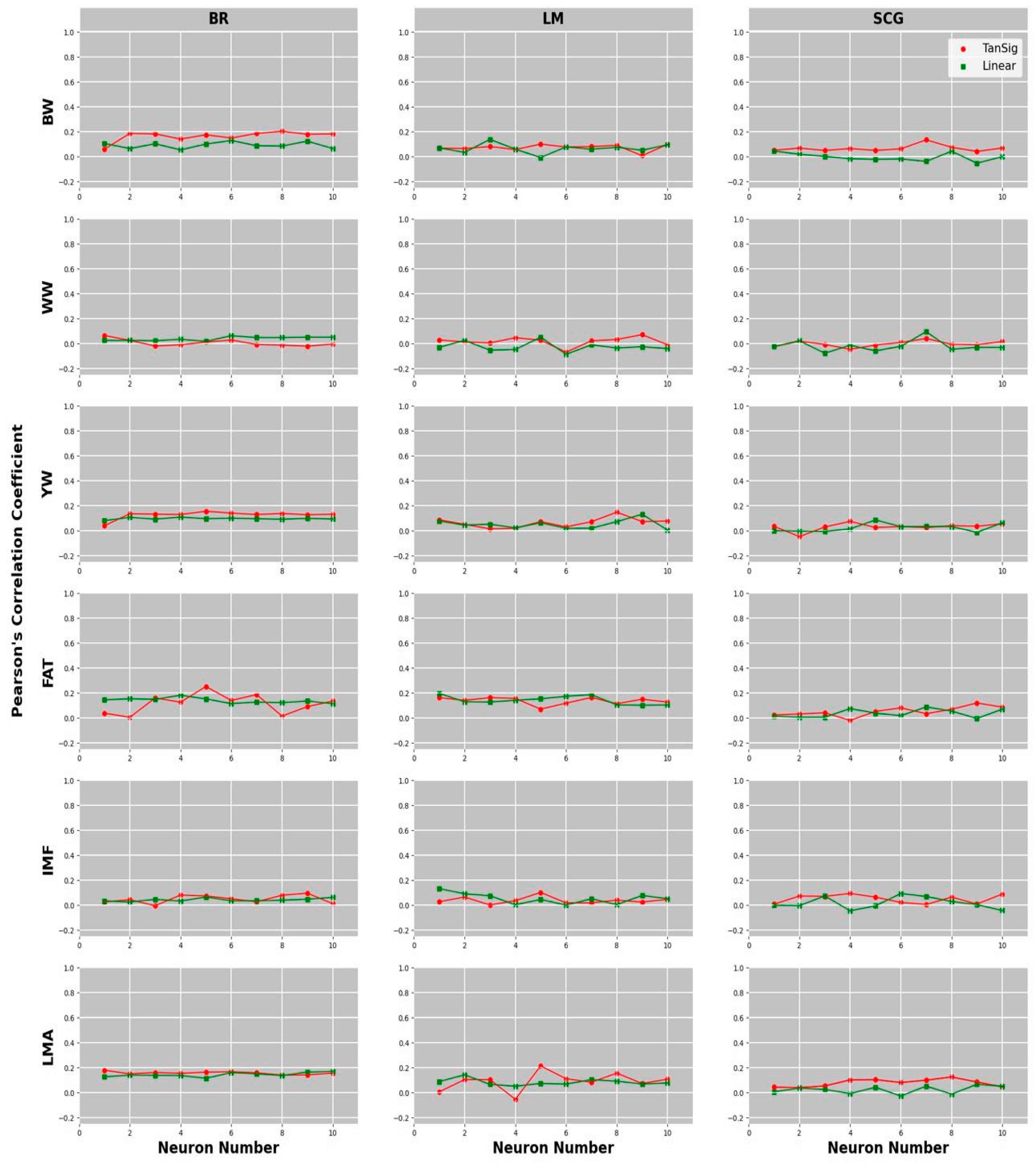
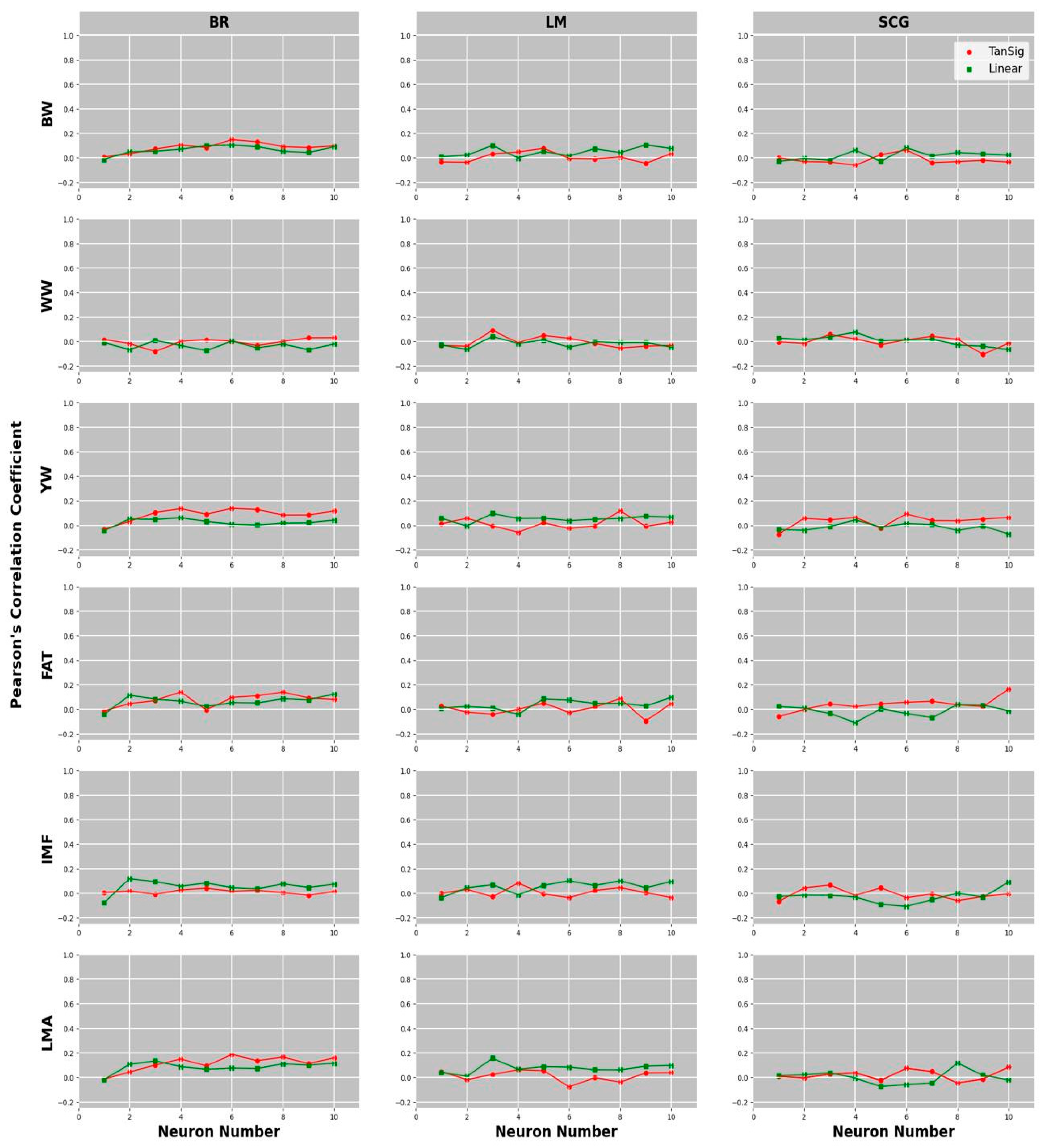
3.2. Comparison of Learning Algorithms and Transfer Functions for the Predictive Ability of MLPANN Models

The predictive performance of MLPANN models depends on the number of neurons in the hidden layer, learning algorithms and the type of transfer functions. Pearson’s correlation coefficients for the predictive performance of MLPANN models are given across different numbers of neurons for learning (BR, LM and SCG) algorithms and transfer (tangent sigmoid and linear) functions, with the univariate analysis presented in Figure 3 and the multivariate analysis in Figure 4.

The predictive performance of MLPANN models was expected to show an increasing trend across the number of neurons in the hidden layer. However, as seen in Figure 3 and Figure 4, there were no increasing trends but fluctuations in the predictive performances of MLPANN models with an increasing number of neurons across different learning algorithms and transfer functions in the univariate and multivariate analysis. There was also no specific number of neurons providing high predictive performance for MLPANN models in the univariate and multivariate analysis. These inconsistent predictive performances of MLPANN models indicated the necessity of a large number of neurons for learning data specifications in the application of ANNs. Okut et al. [37], comparing the predictive ability of different 1-7-neuron ANN models with BR learning algorithms, indicated that the predictive ability of the five-neuron network attained the highest Pearson’s correlation coefficient in the test data, although differences among networks were negligible. Peters et al. [32] showed that predictive performance of 1-10-neuron MLPANN models increased with the number of neurons. However, there was no consistent increase in predictive performance across the number of neurons, which indicated that a small number of neurons would not be enough to learn the specifications of data and would cause an under-fitting problem. Although a large number of neurons is needed to learn the relevant details of data in MLPANN applications, our MLPANN predictive performance results in Figure 3 and Figure 4 were also found to be similar across the number of neurons in the univariate and multivariate analysis of growth and carcass traits. Ehret et al. [18], Gianola et al. [43] and Sinecen [44] showed that ANN models minimally differed in predictive performance across the number of neurons when the genomic relationship $\mathit{G}$ matrix was used. Peters et al. [32] indicated that the ANN predictive performance remained consistent when the sample size was equal to or higher than the number of features of the network.

In this study, BR, LM and SCG backpropagation learning algorithms were used to determine the MLPANN learning algorithm producing better estimates in the univariate and multivariate analyses of growth and carcass traits. Pearson’s correlation coefficients from MLPANN models with BR, LM and SCG learning algorithms were given in columns within Figure 3 and Figure 4 to determine the learning algorithm producing better estimates in the univariate and multivariate analyses of growth and carcass traits. As seen in Figure 3 and Figure 4, Pearson’s correlation coefficients ranged from −0.02 to 0.250 for BR, −0.087 to 0.212 for LM and −0.079 to 0.133 for SCG learning algorithms in the univariate analysis; they ranged from −0.08 to 0.186 for BR, −0.096 to 0.156 for LM and −0.111 to 0.164 for SCG learning algorithms in the multivariate analysis, respectively. Paired-sample t-test indicated that the predictive performances of BR, LM and SCG learning algorithms in the univariate analysis were significantly higher than those of BR, LM and SCG learning algorithms in the multivariate analysis (p-value < 0.01).

In the univariate and multivariate analyses, MLPANN models with the BR learning algorithm resulted in statistically better predictive performances compared to MLPANN models with LM and SCG algorithms (p-value < 0.01). Also, more consistent predictive performances of MLPANN models across the number of neurons were obtained in the BR learning algorithm. Results from the BR learning algorithm are consistent with those of Okut et al. [37], who demonstrated that the predictive performance of ANN models did not depend on network architecture when the sample size was larger than the number of features in the analysis. Our results also agreed with those of Ehret et al. [18], who used the $\mathit{G}$ matrix as an input to the network, and those of Gianola et al. [43], who used Bayesian regularized artificial networks for genome-enabled predictions of milk traits in Jersey cows. Peters et al. [45] compared the MLPANN models with BR, LM and SCG learning algorithms for the analysis of antler beam diameter and length from white-tailed deer and found that the MLPANN model with a BR learning algorithm showed better agreement of the predicted and observed values of antler beam diameter and length; however, the MLPANN model with a SCG learning algorithm resulted in the highest error within the models. Kayri [46] compared ANN models with BR and LM learning algorithms in the analysis of social data and found that the BR learning algorithm with the higher Pearson’s correlation coefficient indicated better predictive performance than the LM learning algorithm. Okut et al. [47] investigated the predictive performance of BR and SCG learning algorithms and found that the ANN model with the BR learning algorithm gave a slightly better performance. In the studies of Bruneau and McElroy [48], Saini [49], Laurent et al. [50] and Ticknor [51], the BR learning algorithm also yielded a moderate or better predictive performance compared to the other learning algorithms.

ANN models are usually applied in univariate analysis and result in similar and consistent predictive performances across learning algorithms and transfer functions [18,45,47]. However, as seen in Figure 4, Pearson’s correlation coefficients from the multivariate analysis indicated that predictive performances of MLPANN models with BR, LM and SCG learning algorithms were different, inconsistent across growth and carcass traits, the number of neurons and transfer functions and worse than those from the univariate analysis. Training in the ANN model is an iterative learning process, and at each iteration, the weights from the input layer to the hidden layer (${\alpha }_j$) and from the hidden layer to the output layer ($w_t$) of the ANN model (Figure 1) are adjusted by using a learning algorithm (BR, LM and SCG) [18] to minimize the difference (the error) between observed and predicted phenotypes [52]. Since six growth (BW, WW and YW) and carcass (FAT, IMF and LMA) traits were analyzed together using the MLPANN models with BR, LM and SCG learning algorithms in the multivariate analysis, the increasing number of features of the MLPANN model and the underlying (positive/negative) genetic relationships among traits affected the iterative learning process of BR, LM and SCG learning algorithms within the neural network and resulted in the lower predictive performance of MLPANN models with BR, LM and SCG learning algorithms in the multivariate analysis.

Transfer functions are an essential part of ANN models, helping with learning and making sense of non-linear and complicated mappings between inputs (genomic relationship) and corresponding outputs (the value of trait or phenotype) [52]. Applying sigmoidal-type, linear transfer functions in the hidden and output layers may be useful when it is necessary to extrapolate beyond the range of training data [53,54]. In this study, two combinations of transfer functions (tangent sigmoid–linear and linear–linear) were used in the hidden–output layers (Figure 1). For the predictive performances of MLPANN models with a tangent sigmoid–linear or linear–linear transfer function combination, Pearson’s correlation coefficients for the tangent sigmoid–linear (red line) or linear–linear (green line) transfer function combination were given based on growth and carcass traits and BR, LM and SCG learning algorithms in univariate (Figure 3) and multivariate (Figure 4) analyses. As seen in Figure 3 and Figure 4, Pearson’s correlation coefficients indicated that the predictive performances of MLPANN models with a tangent sigmoid–linear or linear–linear transfer function combination in the univariate analysis were statistically better than those in the multivariate analysis (p-value < 0.05). In addition, the predictive performances of tangent sigmoid–linear and linear–linear transfer function combinations within univariate and multivariate analyses were different across growth and carcass traits and BR, LM and SCG learning algorithms.

In the univariate analysis, the predictive performances of MLPANN models with the tangent sigmoid–linear transfer function combination for each trait were better than or similar to those of MLPANN models with the linear–linear transfer function combination across learning algorithms. MLPANN models with the tangent sigmoid–linear or linear–linear transfer function combination in the BR learning algorithm resulted in higher predictive performances than those in LM and SCG learning algorithms. Also, the predictive performances of transfer function combinations were more consistent in the BR learning algorithm compared to those in LM and SCG learning algorithms. However, in the multivariate analysis, MLPANN models with the tangent sigmoid–linear or linear–linear transfer function combination in BR, LM and SCG learning algorithms yielded lower predictive performances than those in the univariate analysis. As indicated by Ehret et al. (2015) [18], the complex architectures of MLPANN models and the underlying genetic relationships among growth and carcass traits in the multivariate analysis could cause worse predictive performances by learning irrelevant details of the data.

4. Conclusions

The results from this study showed that 1-10-neuron MLPANN models with the BR, LM and SCG learning algorithms based on tangent sigmoid–linear and linear–linear transfer function combinations and GBLUP models in the univariate analysis of growth and carcass traits resulted in better predictive performances than those of GBLUP and MLPANN models in the multivariate analysis. In the univariate analysis, 1-10-neuron MLPANN models with the BR learning algorithm based on the tangent sigmoid–linear or linear–linear transfer function combination yielded higher predictive performances than those in LM and SCG learning algorithms and GBLUP models. In addition, the predictive performances of MLPANN models with the tangent sigmoid–linear transfer function combination were better than those with the linear–linear transfer function combination in the univariate analysis. The complex architectures of MLPANN models and genetic relationship among growth and carcass traits in the multivariate analysis could have a detrimental effect on the predictive performances of BR, LM and SCG learning algorithms and the tangent sigmoid–linear and linear–linear transfer function combinations. Univariate and multivariate MLPANN models with different numbers of neurons, learning algorithms and transfer functions resulted in slightly higher predictive performance than those of GBLUP models. However, univariate and multivariate GBLUP models were found to be much more computationally efficient than univariate and multivariate MLPANN models in genomic prediction.

References

1. Meuwissen, T.H.E.; Hayes, B.J.; Goddard, M.E. Prediction of total genetic value using genome-wide dense marker maps. Genetics 2001, 157, 1819–1829. [Google Scholar] [CrossRef] [PubMed]
2. Matukumalli, L.K.; Lawley, C.T.; Schnabel, R.D.; Taylor, J.F.; Allan, M.F.; Heaton, M.P.; O’Connell, J.; Moore, S.S.; Smith, T.P.L.; Sonstegard, T.S.; et al. Development and characterization of high density SNP genotyping assay for cattle. PLoS ONE 2009, 4, e5350. [Google Scholar] [CrossRef] [PubMed]
3. Applied Biosystems. Axiom Bovine Genotyping v3 Array (384HT Format). 2019. Available online: https://www.thermofisher.com/order/catalog/product/55108%209#/551089 (accessed on 15 January 2022).
4. Illumina. Infinium iSelect Custom Genotyping Assays. 2016. Available online: https://www.illumina.com/content/dam/illumina-marketing/documents/products/technotes/technote_iselect_design.pdf (accessed on 15 January 2022).
5. Habier, D.; Fernando, R.L.; Kizilkaya, K.; Garrick, D.J. Extension of the Bayesian alphabet for genomic selection. BMC Bioinform. 2011, 12, 186. [Google Scholar] [CrossRef]
6. Pérez, P.; de los Campos, G. Genome-wide regression and prediction with the BGLR statistical package. Genetics 2014, 198, 483–495. [Google Scholar] [CrossRef] [PubMed]
7. Pereira, B.d.B.; Rao, C.R.; Rao, M. Data Mining Using Neural Networks: A Guide for Statisticians, 1st ed.; Chapman and Hall/CRC: London, UK, 2009. [Google Scholar]
8. Kononenko, I.; Kukar, M. Machine Learning and Data Mining: Introduction to Principles and Algorithms; Horwood Publishing: London, UK, 2007. [Google Scholar]
9. Howard, R.; Carriquiry, A.L.; and Beavis, W.D. Parametric and Nonparametric Statistical Methods for Genomic Selection of Traits with Additive and Epistatic Genetic Architectures. G3 Genes Genomes Genet. 2014, 4, 1027–1046. [Google Scholar] [CrossRef]
10. Luna-Nevarez, P.; Bailey, D.W.; Bailey, C.C.; VanLeeuwen, D.M.; Enns, R.M.; Silver, G.A.; DeAtley, K.L.; Thomas, M.G. Growth characteristics, reproductive performance, and evaluation of their associative relationships in Brangus cattle managed in a Chihuahuan Desert production system. J. Anim. Sci. 2010, 88, 1891–1904. [Google Scholar] [CrossRef]
11. Fortes, M.R.S.; Snelling, W.M.; Reverter, A.; Nagaraji, S.H.; Lehnert, S.A.; Hawken, R.J.; DeAtley, K.L.; Peters, S.O.; Silver, G.A.; Rincon, G.; et al. Gene network analyses of first service conception in Brangus heifers: Use of genome and trait associations, hypothalamic-transcriptome information, and transcription factors. J. Anim. Sci. 2012, 90, 2894–2906. [Google Scholar] [CrossRef]
12. Peters, S.O.; Kizilkaya, K.; Garrick, D.J.; Fernando, R.L.; Reecy, J.M.; Weaber, R.L.; Silver, G.A.; Thomas, M.G. Bayesian genome-wide association analysis of growth and yearling ultrasound measures of carcass traits in Brangus heifers. J. Anim. Sci. 2012, 90, 3398–3409. [Google Scholar] [CrossRef]
13. Granato, I.S.C.; Galli, G.; de Oliveira Couto, E.G.; Souza, M.B.E.; Mendonça, L.F.; Fritsche-Neto, R. snpReady: A tool to assist breeders in genomic analysis. Mol. Breed. 2018, 38, 102. [Google Scholar] [CrossRef]
14. Habier, D.; Fernando, R.L.; Dekkers, J.C.M. The impact of genetic relationship information on genome-assisted breeding values. Genetics 2007, 177, 2389–2397. [Google Scholar] [CrossRef]
15. vanRaden, P.M. Efficient methods to compute genomic predictions. J. Dairy Sci. 2008, 91, 4414–4423. [Google Scholar] [CrossRef] [PubMed]
16. Cybenko, G. Approximation by superpositions of a sigmoidal function. Math. Control Signals Syst. 1989, 2, 303–314. [Google Scholar] [CrossRef]
17. Hornik, K.; Stinchcombe, M.; White, H. Multilayer feedforward networks are universal approximators. Neural Netw. 1989, 2, 359–366. [Google Scholar] [CrossRef]
18. Ehret, A.; Hochstuhl, D.; Gianola, D.; Thaller, G. Application of neural networks with back-propagation to genome-enabled prediction of complex traits in Holstein-Friesian and German Fleckvieh cattle. Genet. Sel. Evol. 2015, 47, 22. [Google Scholar] [CrossRef] [PubMed]
19. Haykin, S.S. Neural Networks: A Comprehensive Foundation; Prentice Hall: Hoboken, NJ, USA, 1999; 842p. [Google Scholar]
20. Kröse, B.; Smagt Patrick, V.D. An Introduction to Neural Networks, 8th ed.; The University of Amsterdam: Amsterdam, The Netherlands, 1996; 135p. [Google Scholar]
21. Christodoulou, C.G.; Georgiopoulos, M. Applications of Neural Networks in Electromagnetics, 1st ed.; Artech House: Norwood, MA, USA, 2001; 512p. [Google Scholar]
22. Civco, D.L. Artificial neural networks for land cover classification and mapping. Int. J. Geogr. Inf. Syst. 1993, 7, 173–186. [Google Scholar] [CrossRef]
23. Kaminsky, E.J.; Barad, H.; Brown, W. Textural neural network and version space classifiers for remote sensing. Int. J. Remote Sens. 1997, 18, 741–762. [Google Scholar] [CrossRef]
24. Bouabaz, M.; Hamami, M. A Cost Estimation Model for Repair Bridges Based on Artificial Neural Network. Am. J. Appl. Sci. 2008, 5, 334–339. [Google Scholar] [CrossRef]
25. Dorofki, M.; Elshafie, A.; Jaafar, O.; Karim, O.A.; Mastura, S. Comparison of Artificial Neural Network Transfer Functions Abilities to Simulate Extreme Runoff Data. Int. Proc. Chem. Biol. Environ. Eng. 2012, 33, 39–44. [Google Scholar]
26. Saatchi, M.; McClure, M.C.; McKay, S.D.; Rolf, M.M.; Kim, J.; Decker, J.E.; Taxis, T.M.; Chapple, R.H.; Ramey, H.R.; Northcutt, S.L.; et al. Accuracies of genomic breeding values in American Angus beef cattle using K-means clustering for cross-validation. Genet. Sel. Evol. 2011, 43, 40. [Google Scholar] [CrossRef]
27. Hartigan, J.A.; Wong, M.A.; Algorithm, A.S. 136: A k-means clustering algorithm. Appl. Stat. 1979, 28, 100–108. [Google Scholar] [CrossRef]
28. Gorjanc, G.; Henderson, D.A.; Kinghorn, B.; Percy, A. GeneticsPed: Pedigree and Genetic Relationship Functions. R Package Version 1.52.0. 2020. Available online: https://rgenetics.org (accessed on 15 March 2023).
29. Kassambara, A.; Mundt, F. factoextra: Extract and Visualize the Results of Multivariate Data Analyses. R Package Version 1.0.5. 2017. Available online: https://CRAN.R-project.org/package=factoextra (accessed on 15 March 2023).
30. Demuth, H.; Beale, M. Neural Network Toolbox User’s Guide Version 4.0; The Mathworks: Natick, MA, USA, 2000. [Google Scholar]
31. Su, G.; Christensen, O.F.; Janss, L.; Lund, M.S. Comparison of genomic predictions using genomic relationship matrices built with different weighting factors to account for locus-specific variances. J. Dairy Sci. 2014, 97, 6547–6559. [Google Scholar] [CrossRef]
32. Peters, S.; Sinecen, M.; Kizilkaya, K.; Thomas, M. Genomic prediction with different heritability, QTL and SNP panel scenarios using artificial neural network. IEEE Access 2020, 8, 147995–148006. [Google Scholar] [CrossRef]
33. Peters, S.O.; Kizilkaya, K.; Sinecen, M.; Metav, B.; Thiruvenkadan, A.K.; Thomas, M.G. Genomic Prediction Accuracies for Growth and Carcass Traits in a Brangus Heifer Population. Animals 2023, 13, 1272. [Google Scholar] [CrossRef]
34. Daetwyler, H.D.; Pong-Wong, R.; Villanueva, B.; Woolliams, J.A. The impact of genetic architecture on genome-wide evaluation methods. Genetics 2010, 185, 1021–1031. [Google Scholar] [CrossRef] [PubMed]
35. Zhang, Z.; Liu, J.; Ding, X.; Bijma, P.; de Koning, D.-J.; Zhang, Q. Best linear unbiased prediction of genomic breeding values using a trait-specific marker-derived relationship matrix. PLoS ONE 2010, 5, e12648. [Google Scholar] [CrossRef]
36. Peters, S.O.; Kizilkaya, K.; Sinecen, M.; Thomas, M.G. Multivariate Application of Artificial Neural Networks for Genomic Prediction. In Proceedings of the World Congress on Genetics Applied to Livestock Production, Rotterdam, The Netherlands, 3–8 July 2022. [Google Scholar]
37. Okut, H.; Gianola, D.; Rosa, G.J.M.; Weigel, K.A. Prediction of body mass index in mice using dense molecular markers and a regularized neural network. Genet. Res. 2011, 93, 189–201. [Google Scholar] [CrossRef] [PubMed]
38. Herring, W.; What Have We Learned About Trait Relationships. 2003. 1–8. Available online: https://animal.ifas.ufl.edu/beef_extension/bcsc/2002/pdf/herring.pdf (accessed on 15 March 2023).
39. Peters, S.O.; Kizilkaya, K.; Garrick, D.; Reecy, J. PSX-9 Comparison of single- and multiple-trait genomic predictions of cattle carcass quality traits in multibreed and purebred populations. J. Anim. Sci. 2024, 102 (Suppl. S3), 453–454. [Google Scholar] [CrossRef]
40. Rostamzadeh Mahdabi, E.; Tian, R.; Li, Y.; Wang, X.; Zhao, M.; Li, H.; Yang, D.; Zhang, H.; Li, S.; Esmailizadeh, A. Genomic heritability and correlation between carcass traits in Japanese Black cattle evaluated under different ceilings of relatedness among individuals. Front. Genet. 2023, 14, 1053291. [Google Scholar] [CrossRef]
41. Weik, F.; Hickson, R.E.; Morris, S.T.; Garrick, D.J.; Archer, J.A. Genetic Parameters for Growth, Ultrasound and Carcass Traits in New Zealand Beef Cattle and Their Correlations with Maternal Performance. Animals 2022, 12, 25. [Google Scholar] [CrossRef]
42. Caetano, S.L.; Savegnago, R.P.; Boligon, A.A.; Ramos, S.B.; Chud, T.C.S.; Lôbo, R.B.; Munari, D.P. Estimates of genetic parameters for carcass, growth and reproductive traits in Nellore cattle. Livest. Sci. 2013, 155, 1–7. [Google Scholar] [CrossRef]
43. Gianola, D.; Okut, H.; Weigel, K.; Rosa, G. Predicting complex quantitative traits with Bayesian neural networks: A case study with Jersey cows and wheat. BMC Genet. 2011, 12, 87. [Google Scholar] [CrossRef] [PubMed]
44. Sinecen, M. Comparison of genomic best linear unbiased prediction and Bayesian regularization neural networks for genomic selection. IEEE Access 2019, 7, 79199–79210. [Google Scholar] [CrossRef]
45. Peters, S.O.; Sinecen, M.; Gallagher, G.R.; Lauren, A.P.; Jacob, S.; Hatfield, J.S.; Kizilkaya, K. Comparison of Linear Model and Artificial Neural Network Using Antler Beam Diameter and Length of White-Tailed Deer (Odocoileus virginianus) Dataset. PLoS ONE 2019, 14, e0212545. [Google Scholar] [CrossRef]
46. Kayri, M. Predictive Abilities of Bayesian Regularization and LevenbergMarquardt Algorithms in Artificial Neural Networks: A Comparative Empirical Study on Social Data. Math. Comput. Appl. 2016, 21, 20. [Google Scholar] [CrossRef]
47. Okut, H.; Wu, X.L.; Rosa, G.J.M.; Bauck, S.; Woodward, B.W.; Schnabel, R.D.; Taylor, J.F.; Gianola, D. Predicting expected progeny difference for marbling score in Angus cattle using artificial neural networks and Bayesian regression models. Genet. Sel. Evolut. 2013, 45, 34. [Google Scholar] [CrossRef] [PubMed]
48. Bruneau, P.; McElroy, N.R. LogD7.4 modeling using Bayesian regularized neural networks assessment and correction of the errors of prediction. J. Chem. Inf. Model. 2006, 46, 1379–1387. [Google Scholar] [CrossRef]
49. Saini, L.M. Peak load forecasting using Bayesian regularization, Resilient and adaptive backpropagation learning based artificial neural networks. Electr. Power Syst. Res. 2008, 78, 1302–1310. [Google Scholar] [CrossRef]
50. Lauret, P.; Fock, F.; Randrianarivony, R.N.; Manicom-Ramsamy, J.F. Bayesian Neural Network approach to short time load forecasting. Energy Convers. Manag. 2008, 5, 1156–1166. [Google Scholar] [CrossRef]
51. Ticknor, J.L. A Bayesian regularized artificial neural network for stock market forecasting. Expert Syst. Appl. 2013, 14, 5501–5506. [Google Scholar] [CrossRef]
52. Gurney, K. An Introduction to Neural Networks, 1st ed.; CRC Press: London, UK, 1997. [Google Scholar]
53. Sharma, S.; Sharma, S.; Athaiya, A. Activation functions in neural networks. Int. J. Eng. Appl. Sci. Technol. 2020, 4, 310–316. [Google Scholar] [CrossRef]
54. Maier, H.R.; Dandy, C.G. Neural networks for the prediction and forecasting of water resources variables: A review of modelling issues and applications. Environ. Model. Softw. 2000, 15, 101–124. [Google Scholar] [CrossRef]
Figure 1. Graphical representation of the univariate and multivariate multi-layer perceptron artificial neural networks for the inputs of the additive genomic relationships ( g i j ) between animals from the G matrix and the output of the univariate ( y ^ k ) or multivariate ( y ^ ) predicted values of phenotypes ( y ) by the network where k = { B W ,   W W ,   Y W ,   F A T ,   I M F , L M A } .
Ruminants 05 00016 g001
Figure 2. Tangent sigmoid and linear transfer functions in the hidden layer during the training process in the MLPANN model. (A,B) show the boundaries of tangent sigmoid and linear transfer functions in the MLPANN model.
Ruminants 05 00016 g002
Figure 3. Comparison of predictive abilities for all scenarios in MLPANN model structure using univariate validation data sets. Growth (BW, WW and YW) and carcass (LMA, IMF and FAT) traits are in the rows, while BR, LM and SCG learning algorithms are shown in columns. Panels show the average Pearson’s correlation coefficients over univariate validation data sets in 10 cross-validation runs on the vertical axis and the number of neurons tested on the horizontal axis. Results of linear–linear (Linear) and tangent sigmoid–linear (TanSig) transfer function combinations are presented in each panel.
Ruminants 05 00016 g003
Figure 4. Comparison of predictive abilities for all scenarios in MLPANN model structure using multivariate validation data sets. Growth (BW, WW and YW) and carcass (LMA, IMF and FAT) traits are in the rows, while BR, LM and SCG learning algorithms are shown in columns. Panels show the average Pearson’s correlation coefficients over multivariate validation data sets in 10 cross-validation runs on the vertical axis and the number of neurons tested on the horizontal axis. Results of linear–linear (Linear) and tangent sigmoid–linear (TanSig) transfer function combinations are presented in each panel.
Ruminants 05 00016 g004