Fundamental Characteristics of Wind Loading on Vaulted-Free Roofs

Abstract

The present paper investigates the fundamental characteristics of wind loading on vaulted (cylindrical) free roofs based on a wind tunnel experiment and a computational fluid dynamics (CFD) analysis using Large Eddy Simulation (LES). In the wind tunnel experiment, wind pressures at many points, both on the top and bottom surfaces of rigid roof models, were measured in a turbulent boundary layer. The wind tunnel models, including the tubing system installed in the roof and columns, were made using a 3D printer, which made the roof thickness as small as 2 mm, whereas the span B was 150 mm and the length L ranged from 150 to 450 mm. The rise-to-span ratio f/B ranged from 0.1 to 0.4. Pressure taps were installed along the center arc and an arc near the roof edge (verge) of an instrumented model with a length-to-span ratio of L/B = 1. The value of L/B of the tested models was changed from 1 to 3 using one or two dummy models, which had the same configuration as that of the instrumented model but no pressure taps. The wind direction θ was changed from 0° (perpendicular to the eaves) to ±90° (parallel to the eaves). The CFD simulation was carried out only for limited cases, that is, f/B = 0.1 and 0.4 and θ = 0° and 45°, considering the computational time. The effects of f/B, L/B, and θ on the mean (time-averaged) and fluctuating wind pressures acting on the roofs were investigated. In particular, the flow mechanism generating large wind forces on the roof was discussed. An empirical formula was provided for the distribution of mean wind force coefficients along the center arc (Line C) at θ = 0° and 30° and along the edge arc (Line E) at θ = 40° for each f/B ratio. Note that these wind directions provided the maximum and minimum mean wind force coefficients within all wind directions for Lines C and E. Furthermore, the maximum and minimum peak wind force coefficients on the two arcs were presented. The effect of turbulence intensity of approach flow on the maximum and minimum peak wind force coefficients was investigated. The experimental results were compared with those estimated using a peak factor approach, which showed a relatively good agreement between them. The data presented here can be used to guide the design of the main wind force-resisting systems and the cladding/components of vaulted-free roofs.

1. Introduction

Vaulted-free roofs, which are generally supported by only columns, are constructed worldwide to provide weather protection and shade in public spaces, such as resting places in parks, sports grounds, and carports. These structures are vulnerable to dynamic wind actions due to their lightweight and flexibility. Therefore, it is very important for structural engineers to consider the wind resistance, particularly to estimate the design wind loads appropriately, when designing such structures. Many studies, mainly experimental ones, have been conducted regarding the wind pressure distributions on enclosed buildings with vaulted roofs (e.g., Qiu et al. [1], Natalini and Natalini [2], Xu et al. [3]). The building codes and standards in many countries have incorporated the results of these studies (e.g., ASCE 7 [4], Australian/New Zealand standard [5], AIJ Recommendations for Loads on Buildings [6], and Tian et al. [7]). In contrast, wind loads on vaulted-free roofs have been studied by only a few researchers. As a result, no specification of wind force coefficient is provided for such free roofs in the building codes and standards. In practical design, the wind loads of vaulted-free roofs are often evaluated based on the external wind pressure coefficients of enclosed cylindrical structures combined with some appropriately assumed internal pressure coefficients (wind pressure coefficients on the bottom surface). However, the wind forces acting on free roofs are quite different from those on enclosed buildings because not only the top surface but also the bottom surface is exposed to turbulent winds in the case of free roofs. The wind load specification for a gable-free roof with the same rise-to-span ratio is sometimes used for estimating the design wind load on a vaulted-free roof. However, the flow around a gable-free roof is different from that around a vaulted-free roof, even if the rise-to-span ratio is the same, particularly regarding the location of flow separation and reattachment, resulting in different wind pressure distributions on the roofs. Therefore, it is required to estimate the design wind loads appropriately to investigate the aerodynamic characteristics of vaulted-free roofs.

Free roofs are categorized into two groups: planar-free roofs and curved free roofs. Wind loads on planar-free roofs were studied by several researchers, e.g., Natalini et al. [8]. The wind force coefficients for designing planar-free roofs are specified in many building codes and standards. On the other hand, only a few studies of wind loading on curved free roofs have been carried out to date. This is probably due to difficulties in making wind tunnel models and measuring wind pressures on both the top and bottom surfaces of the roof at many locations. Among curved free roofs, hyperbolic paraboloid (HP) free roofs are often used for tensioned membrane structures. Colliers et al. [9] proposed a hybrid rapid prototyping methodology by making double-curved structures. Thin models of HP-free roofs were made successfully, and then they measured the mean (time-averaged) wind pressure coefficient distributions on such models in a wind tunnel. In addition, wind loads on curved free roofs with special configurations were measured by Sun et al. [10,11] and Kandel et al. [12]. They measured the distributions of mean and peak wind force coefficients over the whole roof. Ding et al. [13] measured wind pressures on domed free roofs with rise-to-span ratios ranging from 0.1 to 0.4 in a wind tunnel. The wind tunnel models were made by using a 3D printer. The thickness of the roof was as small as 2 mm, whereas the span was 150 mm. A number of pressure taps were distributed along the centerline on the top and bottom surfaces. The pressure distribution on the whole roof was obtained by rotating the model. They discussed the flow mechanism generating large wind forces on the roofs based on the results of a CFD analysis with Large Eddy Simulation (LES). Su et al. [14] investigated the wind loads acting on a large-span vaulted coal shed in a wind tunnel. The effect of gable ventilation was investigated. In addition to a model with solid or porous gable walls, a model without gable walls was also used.

To the authors’ best knowledge, few studies have been made of the wind loads on vaulted-free roofs. The first investigation of wind loads on vaulted-free roofs was carried out by Natalini et al. [15]. Note that several investigations which had been made so far by Argentinian researchers were reviewed in their paper. In their experiment, the rise-to-span ratio, f/B, was fixed to 0.2 as a typical value for this type of free roof. The eaves’ height-to-span ratio, h/B, varied from 0.133 to 0.40, and the length-to-span ratio, L/B, was either 2 or 4. The effects of h/B, L/B, and wind direction θ on the mean wind pressure distribution on the roof were discussed. Uematsu and Yamamura [16] tested four vaulted-free roofs with f/B = 0.1–0.4 and L/B = 1.0 in a turbulent boundary layer. The wind tunnel models were made by using a 3D printer in the same manner as in Ding et al. [13]. The thickness of the roof, including the tubing system, was 2 mm. They measured the net wind pressure (wind force) coefficient distributions along the center arc and an arc close to the verge. They also measured the overall aerodynamic forces and moments using a six-component force balance, in which they used 1 mm-thick rigid models made by using the 3D printer. Based on the results, they proposed wind force coefficients for designing the main wind force resisting systems, focusing on the axial forces induced in the columns as the load effects with an assumption that the roof was rigid and supported by four corner columns. This study was the first challenge that experimentally investigated the wind loads on vaulted-free roofs with a wide range of f/B ratios. Recently, Pagnini et al. [17] measured the mean and peak wind force coefficients on a vaulted-free roof with f/B = 0.25, L/B = 1.25, and h/B = 0.25, which was planned to be constructed at the Genoa University campus in Savona, Italy. In addition to the isolated building case, the practical situation, including the nearby buildings and the topography of the surroundings, was tested. The wind force coefficients for designing the main wind force resisting system and the cladding/components of this free roof were proposed. Ding and Uematsu [18] discussed the design wind force coefficients for the main wind force resisting system of a vaulted-free roof with f/B = 0.1 and L/B = 1 based on the LRC (Load Response Correlation) method proposed by Kasperski [19] in which the focus was on the axial force and bending moment induced in the columns as the load effects with an assumption that the roof was supported by two rigid frames, each of which was constructed of two columns and an arch beam and carried the wind loads acting on the tributary area (half area) of the roof. The experimental results for the maximum and minimum peak wind force coefficients were also provided, which may guide the wind-resistant design of cladding/components of the roof. Regardless of these efforts, there are few studies investigating the fundamental characteristics of wind forces and the flow mechanism generating large wind forces on vaulted-free roofs with a wide range of f/B and L/B.

The main purpose of this study is to provide useful information about the wind loads on vaulted-free roofs with a wide range of f/B and L/B based on a wind tunnel experiment and a CFD analysis using LES. The focus is on the mean wind force coefficients and the maximum and minimum peak wind force coefficients. The former is related to the design of wind loads on the main wind force-resisting systems, while the latter is related to the design of cladding/components of the roofs. The experimental models are basically the same as those used by Uematsu and Yamamura [16]. However, longer models with L/B = 2 and 3 are also tested using dummy models with no pressure taps. The turbulence intensity of the flow used in the present study is somewhat larger than that used in Uematsu and Yamamura [16]. Therefore, the effect of turbulence intensity on the wind force coefficients can be discussed. The method of CFD analysis is similar to that of Ding et al. [13], which was used for investigating the wind pressures on domed-free roofs. It should be noted that this paper is an extended version of our previous one [16], focusing on the fundamental characteristics of wind forces on vaulted-free roofs. For this purpose, a CFD simulation is employed to investigate the flow mechanism that causes large wind forces. The range of parameters affecting the wind forces is expanded. Although the tested cases are limited, this study will provide helpful guidance for the wind-resistant design of the main wind-force-resisting systems and cladding/components of vaulted-free roofs.

This paper is composed of six sections. Following this Section (Introduction), Section 2 describes the implementation of the wind tunnel experiment. The wind pressure distributions on the top and bottom surfaces of vaulted-free roofs were measured. Simultaneous pressure measurements at many taps along two representative arcs are made in a turbulent boundary layer. Then, Section 3 outlines the method of CFD analysis. The CFD analysis is carried out only for representative cases, that is, two f/B ratios (0.1 and 0.4), three L/B ratios (1, 2, and 3), and two wind directions (0° and 45°, with 0° being a wind direction perpendicular to the eaves), considering the computational time. The CFD analysis is validated using a comparison with the experimental results. Section 4 shows a comparison of the present results with previous ones. Section 5 describes the results of the wind tunnel experiment and the CFD analysis. The fundamental characteristics of wind pressures and forces acting on the vaulted-free roofs are investigated. The flow mechanism generating large wind forces on the roof is discussed based on the results of wind pressure distributions and flow visualization. The main focus is on the effects of f/B, L/B, and θ on the mean and peak wind force coefficients as well as on the flow characteristics around the roof. Finally, the main conclusions obtained from this study are summarized in Section 6.

2. Experimental Arrangement and Procedure

2.1. Investigated Building

A vaulted-free roof is the subject of this study, as shown in Figure 1 and

Table 1. Dimensions of the buildings investigated in this study.

f/B	L/B	f (m)	B (m)	L (m)	htop (m)
0.1	1, 2, 3	1.5	15	15, 30, 45	8.8
0.2	1, 2, 3	3.0	15	15, 30, 45	9.5
0.3	1, 2, 3	4.5	15	15, 30, 45	10.3
0.4	1, 2, 3	6.0	15	15, 30, 45	11.0

. The span B is 15 m, and the length L ranges from 15 to 45 m; hence, the L/B ratio ranges from 1 to 3. The rise-to-span ratio, f/B, ranges from 0.1 to 0.4. The mean roof height H is fixed to 8 m regardless of f/B. Therefore, the heights of the rooftop (h_top) and eaves (h) depend on f/B. The range of f/B and L/B, which may affect the wind flow around the roof and the wind pressures on the roof significantly, almost covers the values of practical buildings constructed so far in Japan.

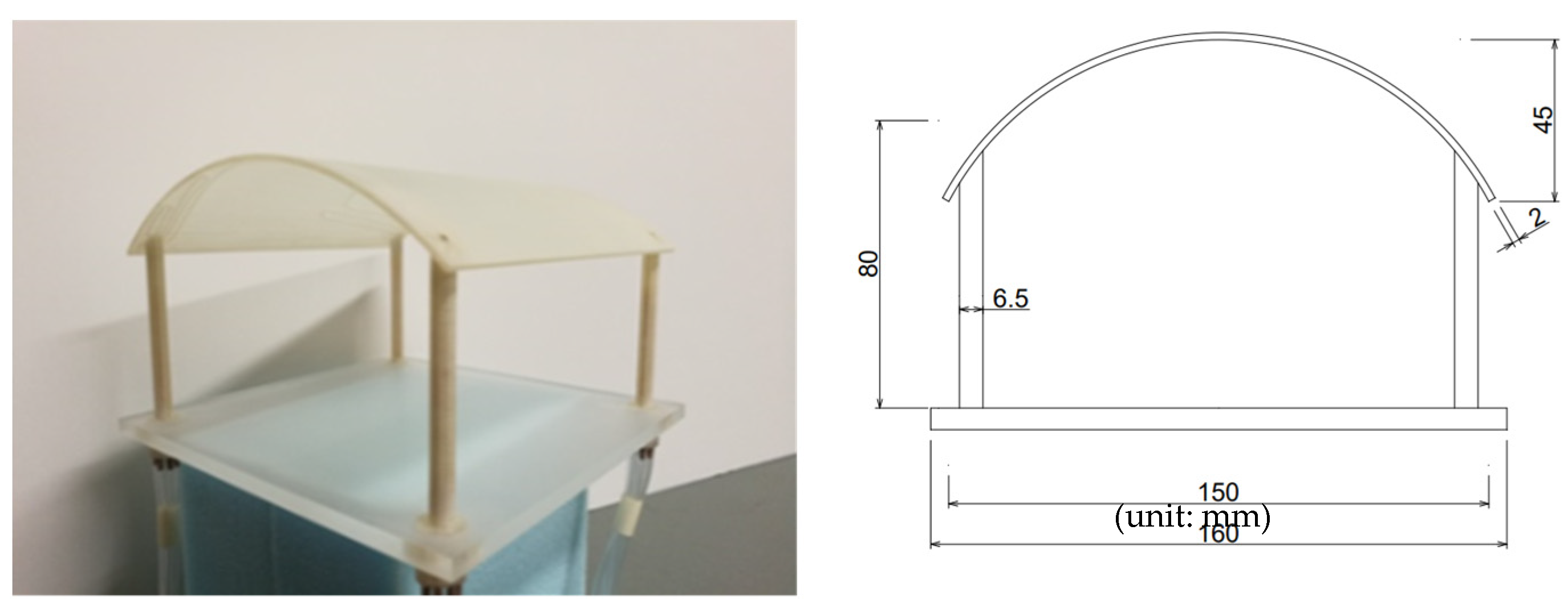
2.2. Wind Tunnel Model

The wind tunnel models were made using a 3D printer with a geometric scale (λ_L) of 1/100. Figure 2 shows an example of an instrumented model with f/B = 0.3 and L/B = 1. Both the roof and the columns, including the tubing system, were integrally formed. The span B and the length L of the instrumented models are both 150 mm. The roof thickness is 2 mm, and the outer diameter of the columns is 6.5 mm. Each instrumented model has seven pressure taps of 0.6 mm diameter both on the top and bottom surfaces along each of the two arcs, Lines C and E, as shown in Figure 3. In the figure, a local coordinate system (ξ,η) is defined. Because the net wind force on a free roof is estimated using the difference between wind pressures on the top and bottom surfaces, it is desirable to set pressure taps at the same location on the top and bottom surfaces. In practice, however, such an instrumentation is impossible for 2 mm thick models. Then, the pressure tap on the bottom surface was located at a point 2 mm away from that on the top surface along the arc, considering that the spatial variation of wind pressures on the bottom surface is smaller than that on the top surface.

In addition to the instrumented model, two dummy models with the same configuration as that of the instrumented model but no pressure taps were also made. Combining the instrumented model with one or two dummy models, the length-to-span ratio, L/B, was changed from 1 to 3, as shown in Figure 4. The location of pressure measuring lines for each model depends on the combination of the instrumented and dummy models. Lines C and E, respectively, represent the center arc and an arc close to the roof edge (verge) in any L/B case. In the cases of L/B = 2 and 3, Line CE represents an arc located about L/2 away from the center arc.

2.3. Wind Tunnel Flow

The experiment was carried out in a turbulent boundary layer developed over the floor of an Eiffel-type wind tunnel at the Department of Architecture and Building Science, Tohoku University, Japan, which had a working section of 1.4 m width, 1.0 m height, and 6.5 m length, by using a standard spire-roughness technique. Figure 5a shows the profiles of mean wind speed U_z and turbulence intensity I_z of the flow at the model’s center without the model in place. In the figure, U_z is normalized by the value U₆₀₀ at a reference height of z = 600 mm, where a pitot static tube was placed. The profile of U_z approximately followed the power law with an exponent of α = 0.27. The value of I_z at the mean roof height H (=80 mm) was approximately 0.2. The normalized power spectrum of wind speed fluctuation at a height of z = 100 mm is shown in Figure 5b. The power spectrum corresponds to the Karman-type spectrum well (an integral length scale of L_x ≈ 0.2 m). According to the AIJ Recommendations for Loads on Buildings [6], the value of L_x is estimated as 58 m at full scale, which corresponds to 0.58 m at model scale, assuming that the geometric scale of wind tunnel flow is 1/100. The value of L_x for the wind tunnel flow is as small as about 1/3 of the target value. However, according to Tieleman et al. [20,21,22], who discussed the similarity of wind tunnel flow required for the wind tunnel experiments investigating the roof wind pressures on low-rise buildings, the L_x value of wind tunnel flow should be larger than 0.2 times the target value and the maximum length of the wind tunnel model. The wind tunnel flow used in the present study almost satisfies Tieleman et al.’s criteria.

The wind speed U_H at the mean roof height H was set to 9 m/s. The Reynolds number Re, defined by $Re=U_{H}H/\nu$, with $\nu$ being the kinematic viscosity of air, was about 4.8 × 10⁵. The blockage ratio Br, defined as the ratio of the model’s vertical cross-section to the wind tunnel’s cross-section, was about 2% at most (in the case of f/B = 0.4 and L/B = 3). As for the values of Re and Br in the present experiment, the requirements of the ASCE Wind Tunnel Testing for Buildings and Other Structures [23], i.e., Br < 5% and Re > 1.1 × 10⁴, were satisfied.

One of the major concerns in the wind tunnel experiments investigating wind loading on a curved structure is the effect of Re on the flow around the structure and the resultant wind pressures on it. This is because the location of flow separation from the structure’s surface is affected by Re significantly. Uematsu and Yamamura [16] investigated the effect of Re on the wind pressure distributions on vaulted-free roofs in a turbulent boundary layer. In their study, Re was defined in terms of U_H and twice the radius of curvature (R) of the roof; the same definition of Re was adopted by Natalini et al. [15]. The reason why they used 2R instead of H as the characteristic length for defining Re was to relate the flow around a vaulted-free roof with that around a circular cylinder, in which the diameter (=twice the radius) of the cylinder is usually used for defining Re. They found that the distribution of mean wind pressure coefficients on the roof was almost independent of Re when Re > 1.0 × 10⁵. Such a feature is consistent with a finding by Macdonald et al. [24] for cylindrical structures; they investigated the effect of Re on the wind pressure distributions on circular cylindrical structures by comparing the wind tunnel results with those obtained from a full-scale measurement of actual silos in natural winds. Macdonald et al. [24] indicated that the wind tunnel experiments conducted at Re > 1.0 × 10⁵ in a turbulent boundary layer might reasonably reproduce a practical full-scale situation. Recently, a similar result was obtained by Liu et al. [25]. In the present experiment, the values of Re defined in terms of U_H and 2R are about 2.53 × 10⁵, 1.41 × 10⁵, 1.09 × 10⁵, and 1.01 × 10⁵ for f/B = 0.1, 0.2, 0.3, and 0.4, respectively. Accordingly, it is expected that the results obtained in the present experiment may reproduce practical conditions almost satisfactorily.

2.4. Experimental Procedure of Pressure Measurements

The design wind speed U_H at the mean roof height H (=8 m) was determined based on the specifications in the AIJ Recommendations for Loads on Buildings [5]. The ‘Basic wind speed’, U₀, was assumed 35 m/s as a representative value for the Main Island of Japan. Note that U₀ corresponds to the 10 min mean wind speed at 10 m above the ground for flat open terrain for the 100-year recurrence. Assuming that the return period is 100 years and the ‘Terrain Category’ is III, which corresponds to suburban exposure, U_H is calculated as 21.3 m/s. Because the mean wind speed at the mean roof height H (=8 cm) in the wind tunnel experiment was 9 m/s, the velocity scale λ_V of wind tunnel flow is calculated as 1/2.4, resulting in the time scale of λ_T (=λ_L/λ_V) = 1/42.

A total of 28 pressure taps installed on the top and bottom surfaces (see Figure 3) were connected to a multi-channel differential pressure transducer (Wind Engineering Institute, MAPS-02) via copper pipes of 1.0 mm inside diameter and flexible vinyl tubes of 1.4 mm inside diameter. The total length of the tubing was about 1 m. The wind pressures at all pressure taps were measured simultaneously at a sampling frequency of 500 Hz, and the sampling time was 14.3 s, which corresponded to 600 s at full scale. A low-pass filter with a cut-off frequency of 300 Hz was applied to eliminate high-frequency electric noise. The distortion of fluctuating wind pressures due to tubing was corrected by using the frequency response function of the tubing system. The measurement was repeated 10 times under each experimental condition. The statistical values of wind pressure coefficients, i.e., mean, standard deviation, and maximum and minimum peak values, were obtained by applying ensemble averaging to the results of 10 consecutive runs. The wind direction θ was defined as shown in Figure 3 and Figure 4, which was changed from −90° to +90° at an increment of 10°. The measurements were also made at two additional wind directions of θ = ±45°.

The wind pressure p acting on the roof was normalized to a wind pressure coefficient C_p as follows:

$$C_p=\frac{p-p_s}{q_H}$$

(1)

where $p_s$ = static pressure measured by the above-mentioned pitot static tube; and $q_H$ = velocity pressure at a height of H (=$\frac{1}{2}\rho U_H^2$, with $\rho$ being the air density). The net wind force is given by the difference between the wind pressures on the top and bottom surfaces. Therefore, the wind force coefficient $C_f$ is defined as follows:

$$C_f=C_{pt}-C_{pb}$$

(2)

where $C_{pt}$ and $C_{pb}$ represent wind pressure coefficients on the top and bottom surfaces, respectively. Thus, the sign of $C_f$ is the same as that of $C_{pt}$.

3. CFD Simulation

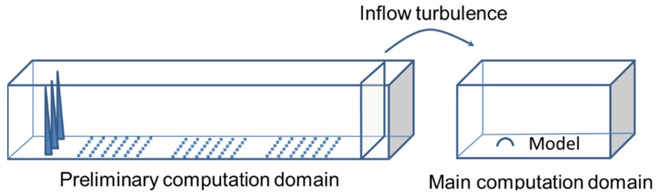
3.1. Computational Model and Domain

The time histories of the wind pressure distributions on and the flow around the vaulted-free roofs are computed using LES. In this study, an open source CFD code ‘OpenFOAM (ver. 2.3.1)’ is used.

The present CFD analysis reproduces the wind tunnel experiment. Thus, the size of the computational model and domain are the same as those of the wind tunnel experiment. The rise-to-span ratio f/B is limited to two values, i.e., 0.1 and 0.4. These two f/B ratios provide representative flow patterns around vaulted-free roofs when the wind direction is nearly normal to the eaves (Uematsu and Yamamura [16]). That is, the flow does not separate from the top surface of the roof when f/B = 0.1, whereas it separates when f/B = 0.4. The computational domain is 1.5 m (=10B) in length, 1.4 m (≈9.3B) in width, and 1.0 m (≈6.7B) in height, as shown in Figure 6. The center of the model is located at 0.475 m (≈3B) leeward from the inlet boundary. The computational grids are arranged as shown in Figure 7, which are generated using software named ‘Pointwise’, where structured and unstructured grids are combined. Three layers of boundary meshes are inserted around the surface of the roof. The total number of grids ranges from about 1.2 to 2.8 million, depending on the f/B ratio. The mesh arrangement was determined based on a comparison of the simulated results with those of the wind tunnel experiment. That is, the mesh arrangement leading to the results most corresponding to those of the wind tunnel experiment was selected. The comparison will be shown in Section 3.3.

3.2. Computational and Boundary Conditions

The LES turbulence model is used. The filtered Navier–Stokes equations are given using the following equations:

$$\frac{𝜕{\overline{u}}_i}{𝜕x_i}=0$$

(3)

$$\frac{𝜕\left({\overline{u}}_i\right)}{𝜕t}+\frac{𝜕\left(\overline{u_i}\overline{u_j}\right)}{𝜕x_j}=-\frac{1}{\rho }\frac{𝜕\overline{p}}{𝜕x_i}+\frac{𝜕}{x_i}\left(\nu \frac{𝜕{\overline{u}}_i}{𝜕x_j}\right)-\frac{𝜕{\tau }_{ij}}{𝜕x_j}$$

(4)

where $\overline{u}$ is filtered velocity, $\overline{p}$ is filtered pressure, ρ is air density, ν is coefficient of viscosity, and ${\tau }_{ij}$ is sub-grid-scale (SGS) stress, which is modeled using a standard Smagorinsky model provided using Equations (5) and (6) [26], which has been applied to many studies on the roof [27,28]. Smagorinsky constant C_s is assumed to be 0.15. The PISO (pressure implicit with the splitting of operators) algorithm is adopted for the pressure–velocity coupling. As for the spatial discretization, the second-order centered difference scheme is used. The second-order implicit scheme is adopted for the time derivative. The computational time T is 15 s, which is equal to 10 min at full scale. The time step is set to $\Delta T=1\times {10}^{-4}$ s.

$${\tau }_{ij}=-2{\left(C_s\overline{\Delta }\right)}^2\left|\overline{S}\right|{\overline{S}}_{ij}$$

(5)

$$\left|\overline{S}\right|=\sqrt{2{\overline{S}}_{ij}{\overline{S}}_{ij}}$$

(6)

The boundary conditions adopted here are summarized in

Table 2. Boundary conditions.

Inlet boundary	Inflow turbulence (Sampling data from preliminary computation)
Outlet boundary	Advective outflow condition
Side and top boundaries	Free-slip condition
Surfaces of ground and roof	No-slip condition

. The inflow turbulence is generated by using a preliminary computation with LES, as shown in Figure 8.

The dimension of the computational domain for the preliminary computation is 5.3 m (length) × 1.4 m (width) × 1.0 m (height), which is almost the same as that of the wind tunnel. The spires and roughness blocks are placed on the floor to generate turbulence, as shown in Figure 8. The computational meshes are arranged as shown in Figure 9. The minimum grid size is 2 mm. The total number of grids is about 7.15 million.

The computational and boundary conditions for the preliminary computation are the same as those for the above-mentioned main computation except for the inlet boundary. A uniform inflow (U = 10 m/s) is given to the inlet boundary. Figure 10 shows the comparison of the profiles of mean wind speed and turbulent intensity at the location of the model’s center with no model in place, which were obtained from the computation and the wind tunnel experiment. It can be found that both results agree relatively well with each other. As for the power spectrum of fluctuating wind at the mean roof height, according to our experience, e.g., Takadate and Uematsu [29], it is expected that the power spectrum of the simulated flow is consistent with the Karman-type spectrum, although the values in a higher reduced frequency range, e.g., fL_x/U_H > 0.1, with L_x being the integral scale of turbulence, are smaller than those of the Karman-type spectrum, due to a filtering effect. In the lower reduced frequency range, the shape of the reduced power spectrum, which is important for discussing the wind loads on buildings, may be generally consistent with that of the Karman-type spectrum. Based on a comparison between the wind tunnel experiment and CFD simulation for the wind pressure coefficient distributions on the roofs (as shown in Figure 11), it is expected that the inflow turbulence generated by the preliminary computation provides an appropriate inflow condition.

3.3. Validation of the CFD Analysis

Figure 11 shows the distributions of the mean wind pressure coefficients on the top and bottom surfaces, ${\overline{C}}_{p,t}$ and ${\overline{C}}_{p,b}$, along Lines C and E when the wind direction is θ = 0°, which were obtained from the CFD analysis and the wind tunnel experiment. In the figure, ‘s’ represents the distance from the leading edge along the arc, normalized by its maximum value, s_max. It can be seen that the agreement between the experiment and CFD analysis is generally good (error < 10%), indicating that the LES used in this study is appropriate.

4. Comparison with Previous Results

Figure 12 shows a comparison of the present experimental results with previous ones by Natalini et al. [15] for the mean wind pressure coefficients, ${\overline{C}}_{pt}$ and ${\overline{C}}_{pb}$, on the top and bottom surfaces. It can be found that the agreement between these two results is relatively good, particularly for ${\overline{C}}_{pb}$ (error < 15%). Some disagreement for ${\overline{C}}_{pt}$ in an area of s/s_max > 0.4 may be due to a difference in the turbulence intensity of the wind tunnel flow and/or some experimental errors; the turbulence intensity at the mean roof height was about 0.2 in the present experiment, while it was about 0.25 in the Natalini et al.’s experiment [15].

5. Results and Discussion

5.1. Mean Wind Pressure and Force Coefficients

5.1.1. General Features

In order to investigate the distributions of mean wind force coefficients ${\overline{C}}_f$ over the whole area, Figure 13 and Figure 14, respectively, show the results of the CFD analysis for θ = 0° and 45°, where the distributions are represented by contour diagrams. Note that Figure 13 shows the results only for the half area considering the symmetry of the model. The numeric characters near the verge and eaves represent the values of the local coordinates, ξ and η, respectively (see Figure 3). When θ = 0°, the contour lines are nearly perpendicular to the wind direction, except for the areas close to the verges (η = 0) in any case of f/B and L/B. The results of a wind tunnel experiment for f/B = 0.2 and L/B = 2–4 conducted by Natalini et al. [16] show a similar tendency. In general, the distribution of mean wind force coefficient is two-dimensional; that is, the variation of ${\overline{C}}_f$ in the η direction is fairly small. Additionally, the magnitude of ${\overline{C}}_f$ on the centerline (Line C) is the largest.

When θ = 45°, on the other hand, the ${\overline{C}}_f$ distribution is rather complicated, particularly in the windward area up to η $\approx$ B/2. Large positive ${\overline{C}}_f$ values (downward) occur near the windward corner (ξ = −B/2, η = 0), while large magnitude negative ${\overline{C}}_f$ values (upward) are induced near the verge in the leeward area (ξ > 0). The largest magnitude of positive (downward) and negative (upward) ${\overline{C}}_f$ values occur on Line E. The ${\overline{C}}_f$ distribution in the windward area up to η $\approx$ B/2 is significantly affected by f/B. However, when the f/B ratio is the same, the distributions for L/B = 1 and 3 are similar to each other. That is, the ${\overline{C}}_f$ distribution in this area is affected by L/B only a little, provided that L/B ≥ 1. The magnitude of ${\overline{C}}_f$ in the leeward area (η > B/2) is relatively small.

The above-mentioned results imply that the distributions of wind force coefficients along Lines C and E represent distinctive features of wind force distributions on vaulted-free roofs. Therefore, the focus is on the distributions along these two lines hereafter.

5.1.2. Effects of f/B and L/B on the Mean Wind Pressure and Force Coefficients

Figure 15 shows the mean wind pressure coefficients, ${\overline{C}}_{pt}$ and ${\overline{C}}_{pb}$, distributed on the top and bottom surfaces, and the resultant mean wind force coefficients ${\overline{C}}_f$ along Line C for various f/B ratios when θ = 0°. Focusing on the distribution of ${\overline{C}}_{pt}$ (Figure 15a), we can find that positive pressures act on a windward area up to s/s_max ≈ 0.2, while negative pressures act widely on the middle and leeward areas, s/s_max > 0.2. The minimum ${\overline{C}}_{pt}$ (maximum |${\overline{C}}_{pt}$|) value generally occurs near the top of the roof, i.e., at s/s_max ≈ 0.5, where the wind speed along the roof becomes the maximum. Note that the increase in wind speed along a convex surface produces a decrease in pressure on the surface according to Bernoulli’s equation. The magnitude of the minimum ${\overline{C}}_{pt}$ increases with an increase in f/B. When f/B = 0.1, the variation of ${\overline{C}}_{pt}$ is relatively small. When f/B = 0.3 and 0.4, on the other hand, the variation is relatively large, and the f/B curve has an inflection point at s/s_max ≈ 0.8 and 0.7 for f/B = 0.3 and 0.4, respectively. Figure 16a,b, respectively, show the distributions of time-averaged streamlines around the roofs with f/B = 0.1 and 0.4 in the (x-z) plane at the mid-span. It can be seen from Figure 16a that the wind flows smoothly along the top surface of the roof without separation when f/B = 0.1. On the other hand, the flow separates from the top surface in the case of f/B = 0.4, as shown in Figure 16b. The point of flow separation roughly corresponds to the inflection point of the ${\overline{C}}_{pt}$ curve. As for the distribution of ${\overline{C}}_{pb}$ (Figure 15b), the ${\overline{C}}_{pb}$ value changes from negative to positive to leeward when f/B = 0.1 and 0.2. It can be seen from Figure 16a that the flow separates downward at the leading edge, resulting in large suctions near the leading edge. The separated flow reattaches on the bottom surface at s/s_max $\approx$ 0.5 when f/B = 0.1. The point of reattachment of the separated flow roughly corresponds to the inflection point of the ${\overline{C}}_{pb}$ curve. The reattached flow generates positive pressures on the bottom surface. In contrast, the separated flow does not reattach on the bottom surface when f/B = 0.4, generating suctions of moderate magnitude over the whole area. It is found that the distribution of ${\overline{C}}_f$ (Figure 15c) is similar to that of ${\overline{C}}_{pt}$ (Figure 15a). This is because the variation of ${\overline{C}}_{pb}$ is so small that ${\overline{C}}_{pt}$ dictates the ${\overline{C}}_f$ distribution. Positive wind forces (downward) act on the windward area, s/s_max < 0.2–0.3, while negative wind forces (upward) act on the middle and leeward areas, s/s_max > 0.2–0.3. The maximum ${\overline{C}}_f$ value occurs at s/s_max $\approx$ 0. The minimum ${\overline{C}}_f$ value occurs in a range of s/s_max = 0.5–0.7, the location of which depends on the f/B ratio.

Figure 17 shows the effects of L/B on the distributions of ${\overline{C}}_{pt}$, ${\overline{C}}_{pb}$ and ${\overline{C}}_f$ along Lines C and E for f/B = 0.1 and L/B = 1–3 when θ = 0°. It can be seen that the effects of L/B on the ${\overline{C}}_{pt}$, ${\overline{C}}_{pb}$, and ${\overline{C}}_f$ distributions are small for both Lines C and E, as might be expected from Figure 13. The same feature was observed for the other wind directions and rise/span ratios, although the results are not shown here to save space. That is, the distributions of mean wind pressure and force coefficients in the area of η < B/2 are affected by L/B only slightly.

5.1.3. Effect of Wind Direction θ on the Mean Wind Pressure and Wind Force Coefficients

Figure 18 shows the effect of wind direction θ on the ${\overline{C}}_{pt}$, ${\overline{C}}_{pb}$ and ${\overline{C}}_f$ distributions along Line C when L/B = 1 and f/B = 0.1 or 0.4. When f/B = 0.1 (Figure 18a–c), both positive and negative values of ${\overline{C}}_{pt}$, ${\overline{C}}_{pb}$, and ${\overline{C}}_f$ decrease in magnitude with an increase in θ. That is to say, the maximum and minimum values of the coefficients among all wind directions occur when θ $\approx$ 0°. The flow mechanism generates the maximum and minimum ${\overline{C}}_f$ values have been explained above. This feature implies that the most critical load condition from the structural viewpoint occurs at θ $\approx$ 0° for lower f/B ratios, such as f/B ≤ 0.2, for example. When f/B = 0.4 (Figure 18d–f), on the other hand, the maximum and minimum ${\overline{C}}_f$ values occur at θ = 30–40°, not at θ $\approx$ 0°. Positive ${\overline{C}}_{pt}$ values in the windward area decrease with an increase in θ. In contrast, the negative ${\overline{C}}_{pb}$ values in the leeward area increase in magnitude with increasing θ; the magnitude becomes the maximum at θ = 30–40°, generating the largest ${\overline{C}}_f$ value (downward) in this area. In such an oblique wind, the flow separates downward at the leading edge and reattaches on the bottom surface of the roof. The reattached flow generates positive pressures on the bottom surface in the leeward area, generating large-magnitude negative ${\overline{C}}_f$ values (upward). As a result, the maximum and minimum ${\overline{C}}_f$ values occur at θ = 30–40°. This feature implies that the most critical load condition from the structural viewpoint occurs at θ = 30–40° for higher f/B ratios, such as f/B ≥ 0.3, for example. Note that the difference in the ${\overline{C}}_f$ distribution between θ = 30° and 40° is relatively small, particularly when the f/B ratio is high.

Figure 19 shows the distributions of ${\overline{C}}_{pt}$, ${\overline{C}}_{pb}$, and ${\overline{C}}_f$ along Line E at various wind directions when L/B = 1 and f/B = 0.1 or 0.4. The distribution at θ = 0° is similar to that along Line C (Figure 17) to some degree. However, in oblique winds (θ = 30–50°), large suctions are generated on the top surface in the leeward area (at s/s_max = 0.6–0.8), as shown in Figure 19a,d. This is because a conical vortex is generated above the top surface due to the flow separation at the windward roof edge (verge). The minimum value of ${\overline{C}}_{pt}$ increases in magnitude as the f/B ratio increases. The value for f/B = 0.4 is about twice that for f/B = 0.1. In such oblique winds, large suctions are generated on the bottom surface in the windward area due to the flow separation at the windward edge. At the same time, positive ${\overline{C}}_{pb}$ values are generated on the bottom surface in the leeward area due to the impinging flow, as shown in Figure 19b,e. The positive ${\overline{C}}_{pb}$ values are rather large when f/B = 0.4. Consequently, large magnitude positive (downward) and negative (upward) wind forces are generated in the windward and leeward half areas, respectively (see Figure 19c,f). The higher the f/B ratio, the larger the magnitude is.

Figure 20 and Figure 21, respectively, show the distributions of time-averaged streamlines in the (x-z) planes along Lines (a) to (c) for f/B = 0.1 and 0.4 when θ = 45°. The results explain the flow mechanisms that cause large magnitude positive and negative wind forces on the roof. The flow does not separate from the top surface when f/B = 0.1 (Figure 20a), whereas it separates upward at the windward edge (verge) and generates a large vortex above the top surface when f/B = 0.4 (see Figure 21a). In general, the higher the f/B ratio, the larger in size the vortex is, and the larger in magnitude the minimum ${\overline{C}}_{pt}$ value is. Meanwhile, as for the bottom surface, the flow separates downward at the windward edge (verge) and reattaches on the bottom surface in the (x-z) plane along Line (b). The separated flow generates suctions on the bottom surface in the windward area, while the reattached and impinging flows generate positive pressures on the bottom surface in the leeward area. In the (x-z) plane along Line (c), the flow separates downward at the windward edge (eave) and generates a separation bubble, which will generate suctions over a wide area.

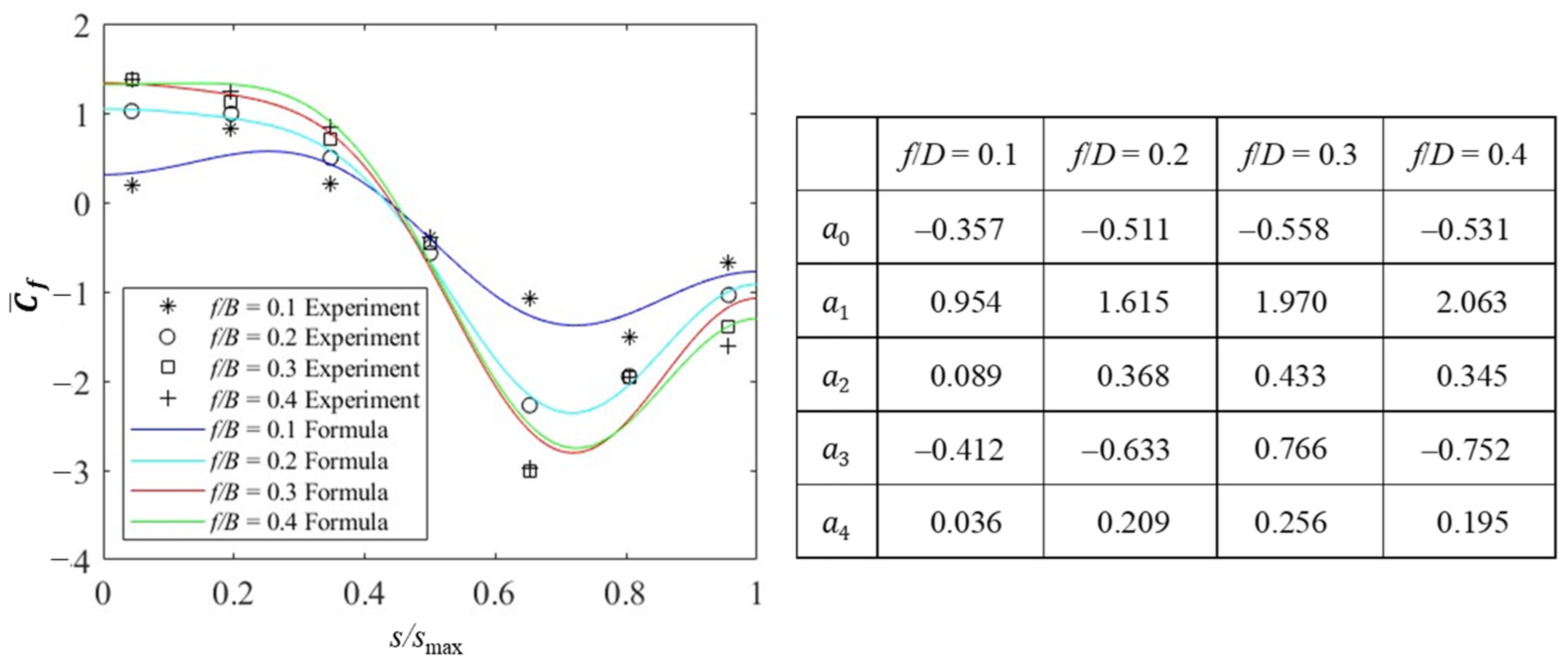
5.1.4. Empirical Formulas for the Mean Wind Force Coefficient Distributions

It may be possible to estimate the design wind loads for the main wind force resisting systems based on the quasi-steady assumption for small-scale structures, such as vaulted-free roofs, investigated in this study. In such a case, the wind force coefficients can be estimated based on the distribution of mean wind force coefficients ${\overline{C}}_f$.

As mentioned above, a normal wind (θ = 0°) or an oblique wind (θ = 30–40°) yields the most critical load condition on Line C, depending on the f/B ratio. Regarding Line E, the most critical load condition is provided by an oblique wind (θ ≈ 40°). Various types of structural systems are used for vaulted-free roofs, among which the simplest one is a system that consists of a series of arch beams arranged in parallel and connected with each other by tie beams. In such a structural system, the design wind loads may be evaluated based on the wind force coefficient distribution along the beam. Then, we propose a model of the ${\overline{C}}_f$ distribution for the above-mentioned three conditions; that is, (1) Line C at θ = 0°, (2) Line C at θ = 30°, and (c) Line E at θ = 40°. The distribution is approximated by the following equation:

$${\overline{C}}_f\left(s\right)={\displaystyle \sum }_{n=0}^4{a}_n\cos \left(n\pi \frac{s}{s_{\max }}\right)$$

(7)

where the coefficients $a_i$ can be determined using the least square method. The empirical formula is compared with the experimental results in Figure 22, Figure 23 and Figure 24. The R-square value for f/B in each case is generally larger than 0.96.

5.2. Maximum and Minimum Peak Wind Force Coefficients

5.2.1. General Features

The purpose of this section is not to propose the wind force coefficients for designing the cladding/components of the roof but to investigate the fundamental characteristics of the maximum and minimum peak wind force coefficients because the number of pressure taps installed on the wind tunnel model is rather limited. Here, we focus on the mean (expected) values of the maximum and minimum peak wind force coefficients, ${\widehat{C}}_f$ and ${\check{C}}_f$, which are gained using ensemble averaging to the results of the ten consecutive runs. Note that the moving averaging time used for evaluating the maximum and minimum peak wind pressure and force coefficients is about 0.25 s at full scale.

Figure 25 and Figure 26 show the most critical values of ${\widehat{C}}_f$ and ${\check{C}}_f$ irrespective of wind direction, ${\widehat{C}}_{f,\mathrm{cr}}$ and ${\check{C}}_{f,\mathrm{cr}}$, along Lines C and E, respectively. As for Line C, very large values of ${\widehat{C}}_{f,\mathrm{cr}}$ occur in the windward area (s/s_max = 0–0.2), which are induced using a combination of large negative pressures owing to flow separation on the bottom surface (see Figure 16a) and large positive pressures owing to flow impinging on the top surface at θ ≈ 0°. On the other hand, ${\check{C}}_{f,\mathrm{cr}}$ becomes very large in magnitude near the top of the roof (s/s_max = 0.5–0.8). The magnitude increases with an increase in f/B. This is due to large suctions induced on the top surface by the flow acceleration at θ ≈ 0° (see Figure 16). The results for Line E are significantly different from those for Line C. The values of ${\widehat{C}}_{f,\mathrm{cr}}$ are almost the same except for an area of s/s_max = 0.8–0.1, irrespective of f/B. The values of ${\check{C}}_{f,\mathrm{cr}}$ range from about −3 to −5 at many pressure taps. Very large absolute values of ${\check{C}}_{f,\mathrm{cr}}$ occur at s/s_max = 0.6–0.7, which are induced using a combination of large suctions on the top surface due to the generation of the conical vortex and large positive pressures due to the flow impinging on the bottom surface in an oblique wind (see Figure 20 and Figure 21). These features of ${\widehat{C}}_{f,\mathrm{cr}}$ and ${\check{C}}_{f,\mathrm{cr}}$ correspond well to those for the mean wind force coefficients described in Section 5.1.2.

It seems interesting to investigate the effect of the turbulence intensity of approach flow on the peak wind force coefficients. Then, the present results for ${\widehat{C}}_{f,\mathrm{cr}}$ and ${\check{C}}_{f,\mathrm{cr}}$ are compared with those of our previous study (Uematsu and Yamamura [16]). The difference between the present and previous experiments is only in the turbulence intensity. In the previous experiment, the turbulence intensity I_H at the mean roof height H was about 0.16, approximately 20% smaller than that of the present experiment. Figure 27 and Figure 28 show comparisons between the present and previous experiments for ${\widehat{C}}_{f,\mathrm{cr}}$ and ${\check{C}}_{f,\mathrm{cr}}$ on Lines C and E, respectively. It is found that the difference is relatively small for Line C. In contrast, we can see a significant difference for Line E; the values of ${\widehat{C}}_{f,\mathrm{cr}}$ and ${\check{C}}_{f,\mathrm{cr}}$ obtained from the present experiment are generally larger in magnitude than those obtained from the previous experiment. Therefore, it may be concluded that the turbulence intensity affects the peak suctions on the top surface due to the generation of a conical vortex and the positive pressures on the bottom surface due to the flow impinging in an oblique wind more significantly.

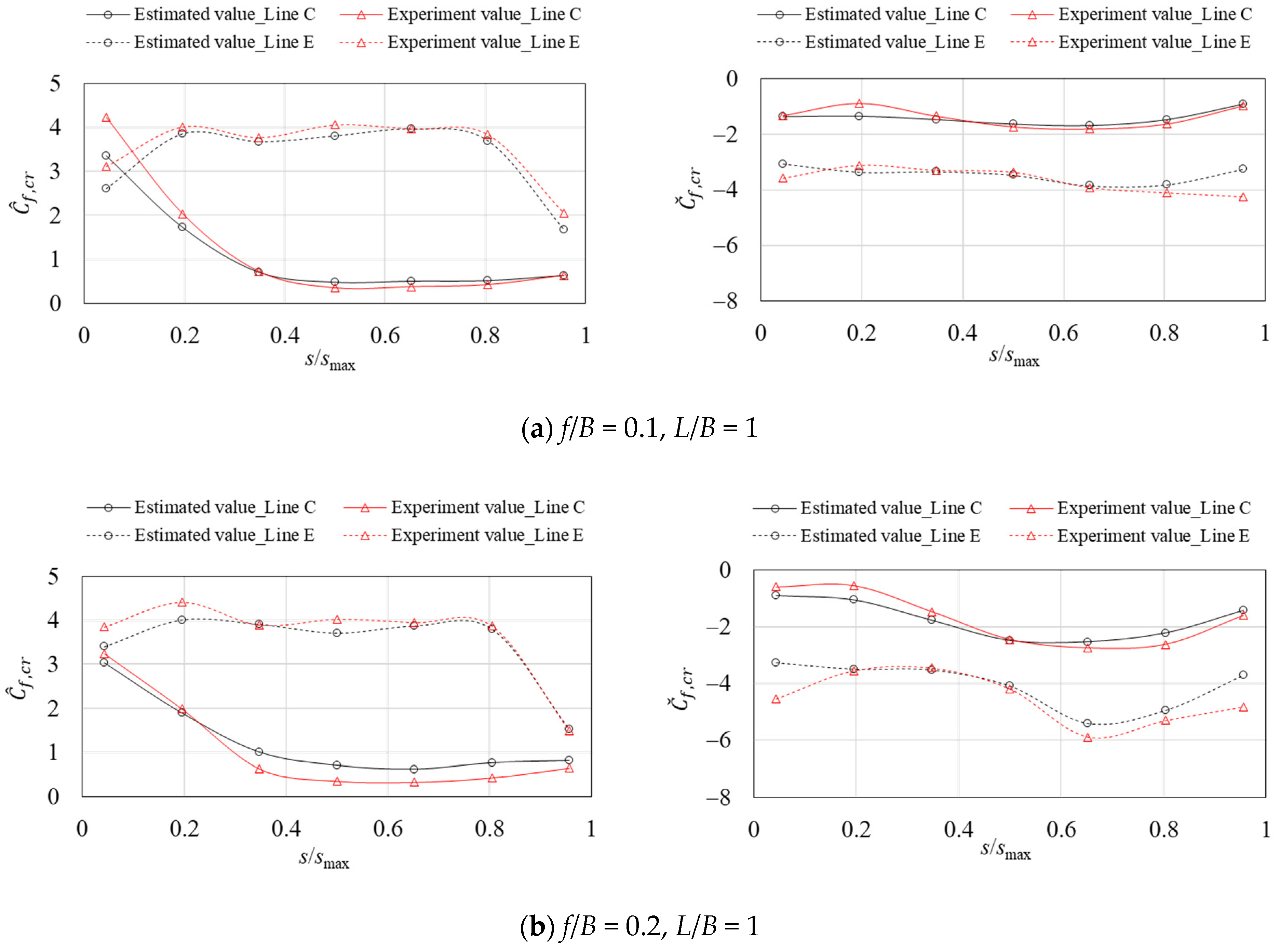
5.2.2. Estimation of the Maximum and Minimum Peak Wind Force Coefficients Based on a Peak Factor Approach

For investigating the wind force distributions in detail, it is necessary to set many pressure taps on both the top and bottom surfaces. In practice, however, making such a wind tunnel model is quite difficult because the roof is supported by only columns. If we measure the wind pressures on only one side (top or bottom surface), we can double the number of pressure taps installed on the surface or the density of pressure taps. In such a situation, the maximum and minimum peak wind force coefficients can be estimated using a combination of the wind pressure coefficients on the top and bottom surfaces measured separately. This sub-section discusses such an estimation method of the maximum and minimum wind force coefficients.

The maximum and minimum peak wind force coefficients, ${\widehat{C}}_f$ and ${\check{C}}_f$, can be estimated as follows based on a peak factor approach:

$${\widehat{C}}_f={\overline{C}}_f+g_f·C_f^{\prime }$$

(8)

$${\check{C}}_f={\overline{C}}_f-g_f·C_f^{\prime }$$

(9)

where ${\overline{C}}_f$ = mean wind force coefficient; $g_f$ = peak factor (assumed 3.5, here); and $C_f^{\prime }$ = RMS fluctuating wind force coefficient. $C_f^{\prime }$ can be provided using the following equation:

$$C_f^{\prime }=\sqrt{C_{pt}^{\prime }{}^2+C_{pb}^{\prime }{}^2-2R_{tb}{C}_{pt}^{\prime }{C}_{pb}^{\prime }}$$

(10)

where $C_{pt}^{\prime }$ and $C_{pb}^{\prime }$ represent the RMS fluctuating wind pressure coefficients on the top and bottom surfaces, respectively, and R_tb is the correlation coefficient between wind pressure fluctuations on the top and bottom surfaces. As mentioned above, large positive wind forces are generated near the windward eaves due to the combination of large positive pressures on the top surface and large suctions on the bottom surface at θ ≈ 0°. Similarly, large peak suctions are generated near the windward verge due to the combination of large positive pressures on the bottom surface and large suctions on the top surface at θ = 30–40°. In such cases, it is thought that the correlation between wind pressures on the top and bottom surfaces is high; that is, large positive pressures on one side and large suctions on the other side occur almost simultaneously, resulting in large wind forces. Thus, it is assumed for simplicity that R_tb = −1.

Figure 29 compares the experimental values with the estimated ones using Equations (8)–(10) for ${\widehat{C}}_{f,\mathrm{cr}}$ and ${\check{C}}_{f,\mathrm{cr}}$ on Lines C and E. It can be seen that the experimental values are close to the estimated values, indicating that the above-mentioned method is effective for estimating the peak wind force coefficients.

6. Concluding Remarks

Fundamental characteristics of flow around and wind loading on vaulted-free roofs have been investigated based on a wind tunnel experiment and a CFD analysis using LES. The effects of rise-to-span ratio f/B, length-to-span ratio L/B, and wind direction θ on the wind pressure and force coefficients on the roof were discussed. The results indicate that the f/B ratio affects the flow and the resulting wind pressures on the roof significantly, whereas the effect of L/B is relatively small.

In a normal wind (θ = 0°), large positive wind forces (downward) are induced near the windward eaves, while large suctions (upward) are induced near the top of the roof. The normal wind produces the largest load effect on the center arc. In an oblique wind (θ = 30–40°), large positive wind forces are induced near the windward corner; on the other hand, large magnitude negative wind forces are induced near the windward verge in the leeward area. Such an oblique wind provides the most critical wind load condition to the edge arc (Line E). The oblique wind also produces large load effects on the arcs located in the windward area up to B/2.

An empirical formula for the distributions of mean wind force coefficients along the center arc (Line C) at θ = 0° and 30° as well as along the edge arc (Line E) at θ = 40° for L/B = 1 was proposed using a Fourier series. The formula can be used for estimating the design wind loads for the main wind force-resisting systems. However, the coefficients were derived from the present wind tunnel experiment with a limited range of parameters. The coefficients a_n may be dependent on such factors as the turbulence intensity of the approach flow. In order to generate the results, the range of parameters should be expanded. This is the subject of our future study.

Furthermore, the characteristics of the most critical maximum and minimum peak wind force coefficients, irrespective of wind direction on Lines C and E, were investigated. The results presented here may provide guidance for the design of cladding/components of the roofs.

References

1. Qiu, Y.; Sun, Y.; Wu, Y.; Tamura, Y. Modeling the mean wind loads on cylindrical roofs with consideration of the Reynolds number effect in uniform flow with low turbulence. J. Wind. Eng. Ind. Aerodyn. 2014, 129, 11–21. [Google Scholar] [CrossRef]
2. Natalini, B.; Natalini, M.B. Wind loads on buildings with vaulted roofs and side walls—A review. J. Wind Eng. Ind. Aerodyn. 2017, 161, 9–16. [Google Scholar] [CrossRef]
3. Xu, Y.; Lyu, X.; Song, H.; Lin, B.; Wei, M.; Yin, Y.; Wang, S. Large-span M-shaped greenhouse with superior wind resistance and ventilation performance. J. Wind Eng. Ind. Aerodyn. 2023, 238, 105410. [Google Scholar] [CrossRef]
4. ASCE/SEI 7-22; Minimum Design Loads and Associated Criteria for Buildings and Other Structures. American Society of Civil Engineers: Reston, VA, USA, 2022.
5. AS/NZS 1170.2; Standards New Zealand, Standards Australia. Australia/New Zealand Standard. 2021. Available online: https://www.standards.govt.nz/shop/asnzs-1170-22021/ (accessed on 30 May 2023).
6. Recommendations of Loads on Buildings; Architectural Institute of Japan: Tokyo, Japan, 2015; Available online: https://www.aij.or.jp/jpn/ppv/pdf/aij_recommendations_for_loads_on_buildings_2015.pdf (accessed on 30 May 2023).
7. Tian, Y.; Guan, H.; Shao, S.; Yang, Q. Provisions and comparison of Chinese wind load standard for roof components and cladding. Structures 2021, 33, 2587–2598. [Google Scholar] [CrossRef]
8. Natalini, B.; Marighetti, J.O.; Natalini, M.B. Wind tunnel modeling of mean pressures on planar canopy roof. J. Wind Eng. Ind. Aerodyn. 2002, 90, 427–439. [Google Scholar] [CrossRef]
9. Colliers, J.; Bollaert, M.; Degroote, J.; Laet, L.D. Prototyping of thin shell wind tunnel models to facilitate experimental wind load analysis on curved canopy structures. J. Wind Eng. Ind. Aerodyn. 2019, 188, 308–322. [Google Scholar] [CrossRef]
10. Sun, X.; Yu, R.; Wu, Y. Investigation on wind tunnel experiments of ridge-valley tensile membrane structures. Eng. Struct. 2019, 187, 104371. [Google Scholar] [CrossRef]
11. Sun, X.; Arjun, K.; Wu, Y. Investigation on wind tunnel experiment of oval-shaped arch-supported membrane structures. J. Wind Eng. Ind. Aerodyn. 2020, 206, 104371. [Google Scholar] [CrossRef]
12. Kandel, A.; Sun, X.; Wu, Y. Wind-induced responses and equivalent static design method of oval-shaped arch-supported membrane structure. J. Wind Eng. Ind. Aerodyn. 2021, 213, 104620. [Google Scholar] [CrossRef]
13. Ding, W.; Wen, L.; Uematsu, Y. Fundamental study of wind loads on domed free roofs. J. Membr. Struct. 2022, 2, 11–19. (In Japanese) [Google Scholar]
14. Su, N.; Peng, S.; Hong, N.; Hu, T. Wind tunnel investigation on the wind load of large-span coal sheds with porous gables: Influence of gable ventilation. J. Wind Eng. Ind. Aerodyn. 2020, 204, 104242. [Google Scholar] [CrossRef]
15. Natalini, M.B.; Morel, C.; Natalini, B. Mean loads on vaulted canopy roofs. J. Wind Eng. Ind. Aerodyn. 2013, 119, 102–113. [Google Scholar] [CrossRef]
16. Uematsu, Y.; Yamamura, R. Wind loads for designing the main wind force resisting systems of cylindrical free-standing canopy roofs, Technical Transactions. Civ. Eng. 2019, 116, 125–143. [Google Scholar]
17. Pagnini, L.; Torre, S.; Freda, A.; Piccardo, G. Wind pressure measurements on a vaulted canopy roof. J. Wind Eng. Ind. Aerodyn. 2022, 223, 104934. [Google Scholar] [CrossRef]
18. Ding, W.; Uematsu, Y. Discussion of design wind loads on a vaulted free roof. Wind 2022, 2, 479–494. [Google Scholar] [CrossRef]
19. Kasperski, M. Extreme wind load distributions for linear and non-linear design. Eng. Struct. 1992, 14, 27–34. [Google Scholar] [CrossRef]
20. Tieleman, H.W.; Reinhold, T.A.; Marshall, R.D. On the wind-tunnel simulation of the atmospheric surface layer for the study of wind loads on low-rise buildings. J. Wind Eng. Ind. Aerodyn. 1978, 3, 21–38. [Google Scholar] [CrossRef]
21. Tieleman, H.W. Pressures on surface-mounted prisms: The effects of incident turbulence. J. Wind Eng. Ind. Aerodyn. 1993, 49, 289–299. [Google Scholar] [CrossRef]
22. Tieleman, H.W.; Hajj, M.R.; Reinhold, T.A. Wind tunnel simulation requirements to assess wind loads on low-rise buildings. J. Wind Eng. Ind. Aerodyn. 1998, 74–76, 675–686. [Google Scholar] [CrossRef]
23. ASCE/SEI 49-12; Wind Tunnel Testing for Buildings and Other Structures. American Society of Civil Engineers: Reston, VA, USA, 2012.
24. Macdonald, P.A.; Kwok, K.C.S.; Holmes, J.D. Wind loads on circular storage bins, silos and tanks: I. Point pressure measurements on isolated structures. J. Wind Eng. Ind. Aerodyn. 1988, 31, 165–188. [Google Scholar] [CrossRef]
25. Liu, L.; Sun, Y.; Su, N.; Wu, Y.; Peng, S. Three-dimensional Reynolds number effects and wind load models for cylindrical storage tanks with low aspect ratios. J. Wind Eng. Ind. Aerodyn. 2022, 227, 105080. [Google Scholar] [CrossRef]
26. Smagorinsky, J. General circulation experiments with the primitive equations: I. The basic experiment. Mon. Weather Rev. 1963, 91, 99–164. [Google Scholar] [CrossRef]
27. Yang, Q.S.; Wang, T.F.; Yan, B.W.; Li, T.; Liu, M. Nonlinear motion-induced aerodynamic forces on large hyperbolic paraboloid roofs using LES. J. Wind Eng. Ind. Aerodyn. 2021, 216, 104703. [Google Scholar] [CrossRef]
28. Yang, Q.S.; Chen, F.X.; Yan, B.W.; Li, T.; Yan, J.H. Effects of free-stream turbulence on motion-induced aerodynamic forces of a long-span flexible flat roof using LES simulations. J. Wind Eng. Ind. Aerodyn. 2022, 231, 105236. [Google Scholar] [CrossRef]
29. Takadate, Y.; Uematsu, Y. Steady and unsteady aerodynamic forces on a long-span membrane structure. J. Wind Eng. Ind. Aerodyn. 2019, 193, 103946. [Google Scholar] [CrossRef]
Figure 1. The subject of this study.
Wind 03 00023 g001
Figure 2. Wind tunnel model (instrumented model) with f/B = 0.3 and L/B = 1.
Wind 03 00023 g002
Figure 3. Pressure taps arrangement on the instrumented model.
Wind 03 00023 g003
Figure 4. Combination of the instrumented and dummy models.
Wind 03 00023 g004
Figure 5. Profiles and power spectrum of the wind tunnel flow.
Wind 03 00023 g005
Figure 6. Computational domain.
Wind 03 00023 g006
Figure 7. Mesh arrangement.
Wind 03 00023 g007
Figure 8. Generation of inflow turbulence.
Wind 03 00023 g008
Figure 9. Mesh arrangement for the preliminary computation.
Wind 03 00023 g009
Figure 10. Comparison between wind tunnel experiment and CFD for the wind profile.
Wind 03 00023 g010
Figure 11. Comparison between the wind tunnel experiment (EXP) and CFD for the mean wind pressure coefficients, C ¯ p t and C ¯ p b , when θ = 0°.
Wind 03 00023 g011
Figure 12. Comparison between the present and previous experiments (Natalini et al. [15]) for the mean wind pressure coefficient distributions along the centerline (f/B = 0.2, L/B = 2).
Wind 03 00023 g012
Figure 13. Distributions of mean wind force coefficients C ¯ f at θ = 0°.
Wind 03 00023 g013
Figure 14. Distributions of mean wind force coefficients C ¯ f at θ = 45°.
Wind 03 00023 g014
Figure 15. Effect of f/B on the mean wind pressure and force coefficients on Line C (L/B = 1, θ = 0°).
Wind 03 00023 g015
Figure 16. Time-averaged streamlines around the roof in the (x, z)-plane at θ = 0°.
Wind 03 00023 g016
Figure 17. Effect of L/B on the distributions of mean wind pressure and force coefficients along Lines C and E (f/B = 0. 1, θ = 0°).
Wind 03 00023 g017
Figure 18. Distributions of mean wind pressure and force coefficients on Line C (L/B = 1).
Wind 03 00023 g018
Figure 19. Distributions of mean wind pressure and force coefficients on Line E (L/B = 1).
Wind 03 00023 g019
Figure 20. Distributions of time-averaged streamlines in the (x, z)-plane (f/B = 0.1, L/B = 1, θ = 45°). (a) Section (a); (b) Section (b); (c) Section (c).
Wind 03 00023 g020
Figure 21. Distributions of time-averaged streamlines in the (x, z)-plane (f/B = 0.4, L/B = 1, θ = 45°). (a) Section (a); (b) Section (b); (c) Section (c).
Wind 03 00023 g021
Figure 22. Empirical formula for the C ¯ f distribution along Line C at θ = 0°.
Wind 03 00023 g022
Figure 23. Empirical formula for the C ¯ f distribution along Line C at θ = 30°.
Wind 03 00023 g023
Figure 24. Empirical formula for the C ¯ f distribution along Line E at θ = 40°.
Wind 03 00023 g024
Figure 25. Most critical values of the maximum and minimum peak wind force coefficients, irrespective of wind direction, C ^ f , cr and C ˇ f , cr , on Line C.
Wind 03 00023 g025
Figure 26. Most critical values of the maximum and minimum peak wind force coefficients, irrespective of wind direction, C ^ f , cr and C ˇ f , cr , on Line E.
Wind 03 00023 g026
Figure 27. Comparison between the present and previous experiments for C ^ f , cr and C ˇ f , cr on Line C.
Wind 03 00023 g027
Figure 28. Comparison between the present and previous experiments for C ^ f , cr and C ˇ f , cr on Line E.
Wind 03 00023 g028
Figure 29. Comparison between experiment and estimation for the maximum and minimum peak wind force coefficients on Lines C and E.
Wind 03 00023 g029aWind 03 00023 g029b