Article

A Statistical–Dynamical Downscaling Technique for Wind Resource Mapping: A Regional Atmospheric-Circulation-Type Approach with Numerical Weather Prediction Modeling

by
Xsitaaz T. Chadee
1,*,
Naresh R. Seegobin
2,† and
Ricardo M. Clarke
1
1
Environmental Physics Lab, Department of Physics, Faculty of Science and Technology, The University of the West Indies, St. Augustine Campus, Circular Road, St. Augustine 330912, Trinidad and Tobago
2
Department of Computing and Information Technology, Faculty of Science and Technology, The University of the West Indies, St. Augustine Campus, Circular Road, St. Augustine 330912, Trinidad and Tobago
*
Author to whom correspondence should be addressed.
Current address: Campus Information Technology Services, The University of the West Indies, St. Augustine Campus, Circular Road, St. Augustine 330912, Trinidad and Tobago.
Submission received: 26 November 2024 / Revised: 19 February 2025 / Accepted: 20 February 2025 / Published: 1 March 2025

Abstract

:
Many Caribbean low-latitude small island states lack wind maps tailored to capture their wind features at high resolutions. However, high-resolution mesoscale modeling is computationally expensive. This study proposes a statistical–dynamical downscaling (SDD) method that integrates an atmospheric-circulation-type (CT) approach with a high-resolution numerical weather prediction (NWP) model to map the wind resources of a case study, Trinidad and Tobago. The SDD method uses a novel wind class generation technique derived directly from reanalysis wind field patterns. For the Caribbean, 82 wind classes were defined from an atmospheric circulation catalog of seven types derived from 850 hPa daily wind fields from the NCEP-DOE reanalysis over 32 years. Each wind class was downscaled using the Weather Research and Forecasting (WRF) model and weighted by frequency to produce 1 km × 1 km climatological wind maps. The 10 m wind maps, validated using measured wind data at Piarco and Crown Point, exhibit a small positive average bias (+0.5 m/s in wind speed and +11 W m−2 in wind power density (WPD)) and capture the shape of the wind speed distributions and a significant proportion of the interannual variability. The 80 m wind map indicates from good to moderate wind resources, suitable for determining priority areas for a detailed wind measurement program in Trinidad and Tobago. The proposed SDD methodology is applicable to other regions worldwide beyond low-latitude tropical islands.

1. Introduction

Wind energy’s role as a protagonist in the energy transition will depend on ensuring the industry’s growth is sustainable, just, and socially responsible while resting on a clear and feasible economic proposition [1]. According to the International Renewable Energy Agency (IRENA) and the International Energy Agency (IEA) roadmaps for a 1.5 °C pathway [2,3], wind energy will become a central pillar of the global energy system by 2050, with more than 8100 GW of wind capacity generating more electricity than any other energy source [2]. There are challenges to ensure wind energy growth over the next few years. Small island developing states (SIDS) could use wind power installations to provide affordable and clean energy (UN Sustainable Development Goal (SDG) 7) to aid in their development and, in the process, contribute to taking action to combat climate change impacts (SDG 13) [4]. However, limited relevant wind data and related suitable approaches to modeling wind flows at high resolutions are some challenges restricting the development of wind potential scenarios in SIDS. SIDS often have sparsely measured datasets to support wind power projects. The World Meteorological Organization (WMO) stations provide climatic data for multiple uses but not for wind power projects. For SIDS to implement fully their nationally determined commitments (NDCs) to the Paris Agreement to mitigate climate change impacts, suitable approaches to prioritize wind potential are required.
For regions with sparse in situ measured datasets, the modern-day approach to wind prospecting or mapping is to model atmospheric flows. The choice of the numerical model depends on the complexity of the terrain. Small islands need non-steady, non-linear models that can simulate thermally driven mesoscale wind circulations, such as sea–land breezes that are prevalent around islands. Of the various models, numerical weather prediction (NWP) models are best suited for modeling atmospheric flows around islands. They model the atmosphere as a fluid and solve the time-dependent equations governing atmospheric dynamics, thermodynamics, and chemical processes, including conservation of mass, momentum, heat, and moisture phases [5]. Together with elevation data, land cover, vegetation indices, sea surface temperatures (SSTs), and soil content, mesoscale NWP models can resolve mesoscale thermally driven wind circulation patterns [5]. In addition, they have been used for preliminary wind resource assessments in several regions [5,6,7,8,9,10,11,12,13,14,15,16,17,18,19].
However, one problem for small island states is that the modeling of winds at appropriate high-resolution scales to capture mesoscale wind circulation, such as sea–land breezes, is computationally expensive. Current modeling strategies tend to compromise by modeling at lower, but still reasonably high, spatial resolutions with NWP models and then drive their outputs with linear models at greater resolutions [20]. However, lower-resolution NWP simulations, even at 3 km × 3 km resolutions used in global wind maps [21], are still too low to resolve mesoscale phenomena around some small islands. In addition, in the current global drive to implement wind turbine technologies to mitigate the impacts of climate change, assessments of the potential changes in wind resources are needed to better optimize the use of energy resources in the future. Developing high-resolution wind climatologies through high-resolution simulations of wind flow for each day with NWP models is computationally infeasible without supercomputing capabilities to achieve results in an acceptable timeframe for advising on policy decisions; SIDS often do not have such supercomputing facilities. The computational expense multiplies for developing wind climatologies for small islands at horizontal spatial resolutions of 1 km × 1 km and higher, where resolving the coastline is important. Past studies have tackled this problem using several wind class generation schemes to reduce large-scale winds into a smaller set of representative wind classes. High-resolution simulations of representative atmospheric states associated with each large-scale wind class and the frequency of occurrence of the wind class have been used in creating wind maps [11,16] and in climate change impact assessments of other variables, such as temperature and precipitation [22,23,24]. This methodology is referred to as statistical–dynamical downscaling (SDD), as it uses representative atmospheric states. These representative atmospheric states are referred to as wind classes when the downscaling process leads to wind maps, also known as wind atlases.
Some wind class generation methodologies determine geostrophic wind speeds and directions from pressure data [16,19] and have worked well for generating wind atlases for mid-latitude areas. However, for low-latitude areas, where most SIDS are located, such wind class generation methods may not be suitable for generating representative wind classes [18], as they tend to overestimate the geostrophic winds. Other wind classification methods may use geostrophic wind speeds directly from reanalysis data, which capture the geostrophic winds of low-latitude areas. However, they may select a typical mean year or a 365-day sample that represents the long-term mean wind speed [25]. These do not typically allow for the temporal representation of the wind resource [18], including assessing the interannual variability in the wind. Interannual variability is important for wind farm developers, as it has a significant impact on the economic feasibility of a wind project; in years of lower power output, income will be reduced, and wind farm developers will need additional financial reserves during these years for sustaining the wind farm. Therefore, it is necessary to project the minimum possible wind resources at a potential wind farm site. To accommodate for the temporal variation in the wind, some researchers have used an empirical orthogonal function (EOF) decomposition technique to derive spatially independent patterns that represent the variability in wind speed and other parameters and a time series based on the principal components [26]. However, the EOF patterns lose information about the actual wind fields.
In this study, we propose a statistical–dynamical downscaling method for generating high-resolution wind maps for SIDS, which are built on an atmospheric-circulation-type catalog defined directly from wind fields provided by reanalysis data. As streamline (wind field) analysis is used to investigate the atmospheric circulation at low latitudes [27], a classification of daily wind field patterns over a region would assist in generating wind classes. An atmospheric-circulation-type (CT) catalog derived from wind fields is suitable for any location, including in low-latitude regions, as it overcomes the limitations of previous classifications based on geostrophic wind estimates. Some wind class methodologies estimate geostrophic wind speeds from pressure data. This typically gives accurate estimates in temperate regions but not in tropical regions, as the geostrophic wind is inversely proportional to the magnitude of the Coriolis force and the sine of the latitude, which approach zero closer to the equator [27]. In tropical regions, the geostrophic balance is less relevant [28]. The wind class generation technique used in this work is based directly on wind field patterns and overcomes this limitation of previous methodologies, as it directly accounts for observed wind behaviors rather than using theoretical estimates. As such, the current SDD method is applicable to any region in addition to low-latitude regions. Furthermore, the interannual variation in the wind is captured using a long-term dataset of reanalysis data to categorize the frequencies of the occurrence of each wind class in each year prior to using a statistical framework. The proposed wind class generation method is outlined in Section 2 and is based on a previous catalog of atmospheric circulation types developed for the Caribbean region [29], as the case study for this work is a Caribbean island state. In Section 2, we describe the NWP model, its configurations, its input data, and the modeling domain. The NWP model used is the Weather Research and Forecasting (WRF) model. The WRF model has been extensively used for mesoscale wind mapping and wind forecasting studies globally [6,20,21,30,31,32,33,34]. In addition, its planetary boundary layer (PBL) configuration was tested for the best PBL scheme that could simulate the local-scale wind speeds and wind speed distributions for the case study in this work, Trinidad and Tobago [35]. In addition, the SDD method in this study uses the statistical framework of Frey-Buness et al. [36] to determine the long-term historical winds and estimate the range of the interannual variability in the wind at the local scale. This statistical framework is described in Section 2, and it demonstrates how the high-resolution NWP simulation for each wind class is combined with a frequency of occurrence to determine the resulting average wind speeds and wind power densities. The SDD method is first validated with local-scale measured data in terms of the historical long-term wind speed average and wind power density at the 10 m level in Section 3. In addition, the ability of the methodology to determine the range of interannual variations is also examined and confirmed before presenting (i) the wind maps for average wind speeds and wind power densities at the 50 m and 80 m levels and (ii) the vertical shear. Concluding remarks are presented in Section 4.

2. Materials and Methods

2.1. Statistical–Dynamical Downscaling Methodology to Develop High-Resolution Wind Maps

The proposed statistical–dynamical downscaling approach to create a wind climatology has three main steps, as shown in Figure 1, and is applied to a case study of the Caribbean islands of Trinidad and Tobago (described in Section 2.2). The first step involves defining the wind classes based on the daily atmospheric circulation types, as defined from a classification of wind fields (Section 2.3). The second step is determining the diurnal variation in high-resolution mesoscale wind fields for the case study islands, using the wind classes as input for a mesoscale numerical weather prediction model (Section 2.4).
In the third, and final, step, the wind climate was calculated by weighting each high-resolution simulation corresponding to a wind class with its corresponding frequency of occurrence. In this last step, the wind probability density function at each grid point is calculated (Section 2.5). Finally, the resulting wind speed and wind power density maps are validated at the locations and heights at which available wind data are collected (Section 2.5).
The proposed SDD approach is applicable to any region, and in this study, it is applied to the island state of Trinidad and Tobago, the southernmost islands of the Caribbean. As such, in step 1, the atmospheric-circulation-type catalog is defined for the Caribbean region.

2.2. Study Region of the Case Study—Location, Climate, and Energy Situation

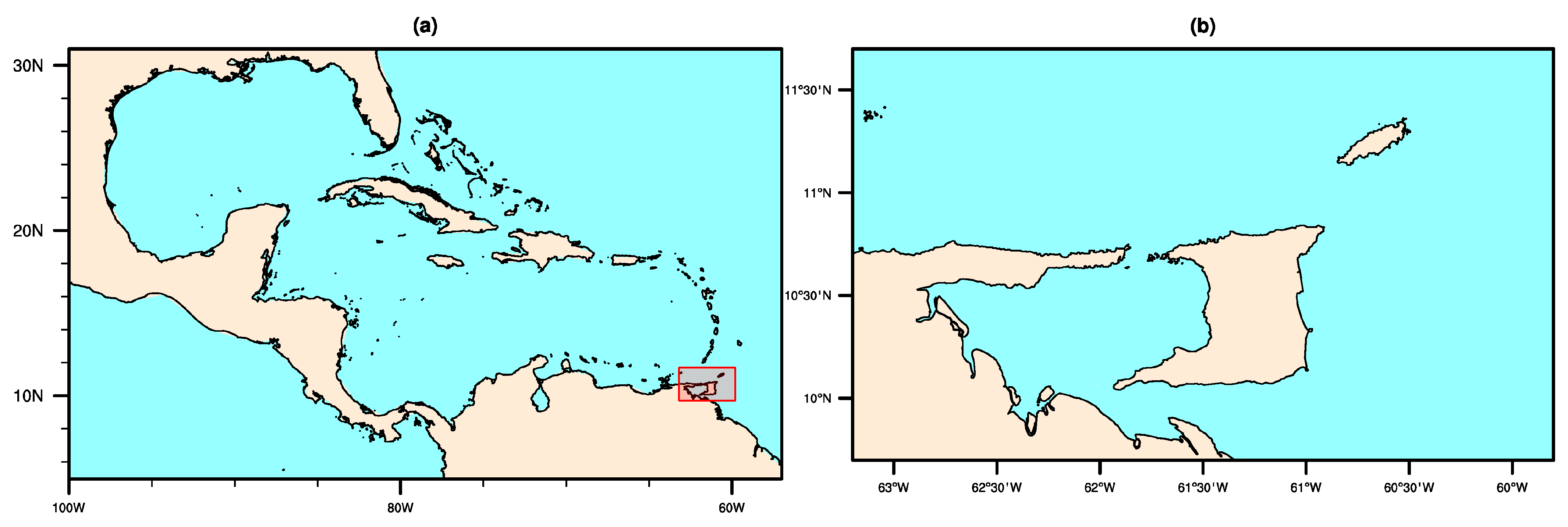
The study region is defined as the area on which the high-resolution wind maps will be produced, the Caribbean islands of Trinidad and Tobago. Trinidad and Tobago is an island state comprising two main islands located at 10° N–11.5° N, 60° W–62° W (Figure 2) at the southernmost end of the Caribbean archipelago and to the northeast of Venezuela (Figure 2a). The two main islands have a total area of approximately 5130 km2, where the larger island, Trinidad, has an area of 4800 km2 [37], and the smaller main island is approximately 316 km2 [38] (Figure 2b). The climate of the islands is defined by its rainfall characteristics, with a dry season from January to May and a wet season from June to December [39]. Trinidad and Tobago is often considered to be ‘lucky’ to be out of the dominant hurricane path because of its low latitude. Nonetheless, the passage of hurricanes is accompanied by heavy rainfall and damaging flooding conditions [40].
The island state is unique in that it is the only small island developing state that actively uses its native oil and natural gas resources, with the energy sector contributing approximately 51% of the total revenue in 2023 [41]. This sector includes both onshore and offshore activities with significant offshore operations, as shown in its energy map (refer to https://ngc.co.tt/wp-content/uploads/2024/01/Energy-Map-of-Trinidad-Tobago-2023.pdf; accessed on 31 January 2025). The island state has been a key player in the world energy market via ammonia and methanol production from its downstream petrochemical industries [42]. In 2021, Trinidad and Tobago was the world’s largest exporter of ammonia, slightly ahead of the Russian Federation and Saudi Arabia [43], and the second largest exporter of methanol in 2022 [44]. However, recent declines in export volumes [45], likely because of shortages in natural gas production [41], have necessitated a diversification in the energy mix to include renewable energy. Solar photovoltaics and wind power have been recognized as the main renewable energy technology alternatives for power generation [41]. Given wind power’s potential to offset all the local power needs, high-resolution wind maps are essential for resource assessment.

2.3. Wind Class Definition from an Atmospheric-Circulation-Type Catalog

In step 1, wind classes are defined from a catalog of atmospheric circulation types. There are three sub-steps for step 1:
1.1: Determining the catalog of the atmospheric circulation types for a region;
1.2: Defining the number of wind classes based on this catalog;
1.3: Assessing the accuracy of the wind classes to reproduce surface-level winds from the input data that will be fed into the numerical weather prediction model.
Figure S1 summarizes the data flow and processing stages for this step. Refer to the Supplementary File for Figure S1.

2.3.1. An Atmospheric Circulation Catalog for the Caribbean

The atmospheric circulation (large-scale prevailing winds) is known to influence regional and local-scale climates [46]. A classification technique, via automated or manual rules, is used to simplify the complex nature of atmospheric circulation to discrete patterns or circulation types [47]. These types are often categorized based on synoptic-scale pressure patterns. However, as this study focuses on wind resources in low-latitude regions, the circulation type is defined as a frequently recurring regional wind pattern.
Atmospheric circulation catalogs are region specific. Although this limits the direct applicability of the SDD method to other regions, it can provide insights into the relationships between atmospheric circulation types and phenomena such as wind energy droughts, surface wind ramp events, and extreme wind events [48,49,50]. Such relationships may be useful in predicting such events and, thus, wind variability to assist in optimizing energy resources to ensure reliable and adequate energy supplies.
Several catalogs have been defined for various regions globally and differ in the variables classified, the classification method, and the domain [51]. For example, the Cost733cat project is a database of 22 catalogs for Europe [52]. The present study uses the Caribbean circulation catalog by Chadee and Clarke [29]. A brief description of the classification variables, method, and domain is provided in this section.
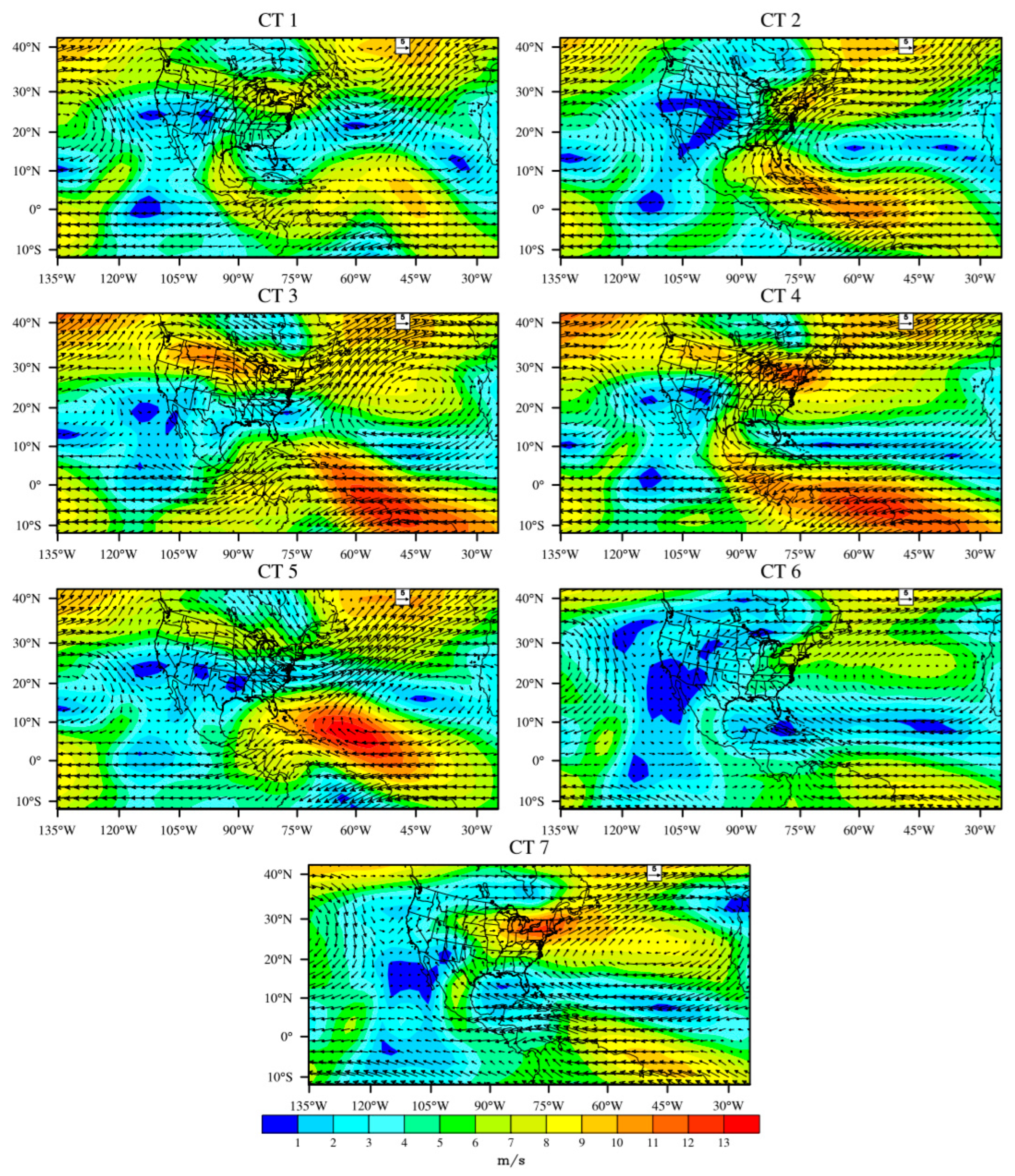
The atmospheric-circulation-type catalog was developed by classifying the 850 hPa daily wind fields over a domain spanning 0° N–30° N and 110° W–40° W. Any reanalysis dataset can provide these wind fields; Chadee and Clarke [29] used the National Center for Environmental Prediction/Department of Energy (NCEP-DOE) reanalysis data, available for a 2.5° × 2.5° horizontal-resolution grid. The daily wind fields for a thirty-two-year period (1 January 1979 to 31 December 2010) were classified using Ward’s hierarchical clustering scheme followed by a k-means partitional clustering scheme. The number of atmospheric circulation types was determined by identifying step changes in the within-cluster sum of squares [29]. Seven frequently occurring atmospheric circulation types (CTs) were identified for the Caribbean region (Figure 3) [29]. A detailed methodology and the properties of these frequently occurring CTs can be found in [29].

2.3.2. Defining the Wind Classes from the Atmospheric Circulation Types

After identifying the number of atmospheric circulation types representing a region’s atmospheric circulation, the wind classes are defined as the typical monthly wind-field pattern of each circulation type. The typical pattern of each CT in each month was found by determining the pattern closest to the mean monthly wind field for each CT. As seven atmospheric circulation types were previously determined for the Caribbean, there should be eighty-four classes when the representations of each circulation type (CT) are considered in each month. However, two types (CT 4 and CT 5) never occur in August [29].
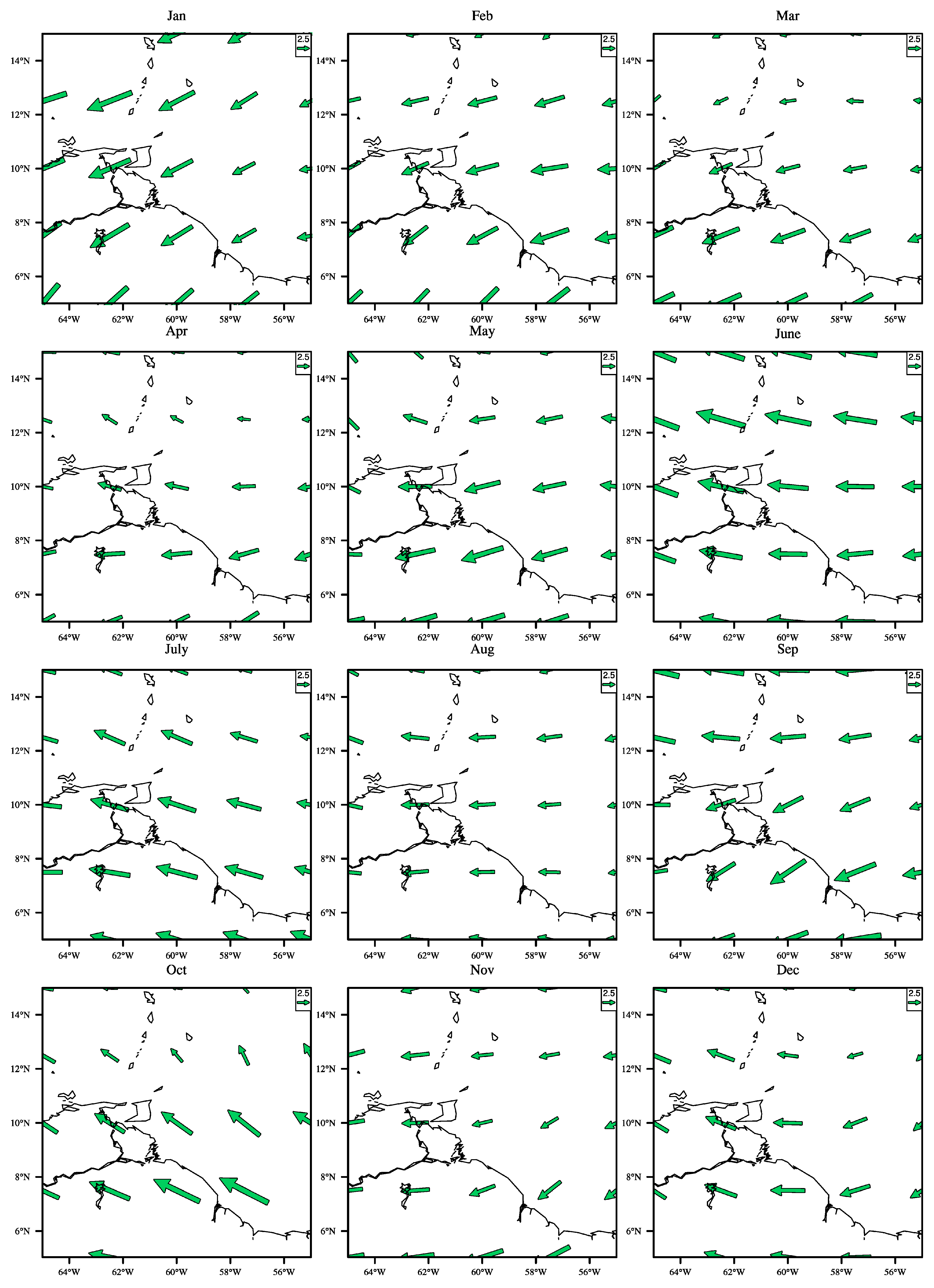
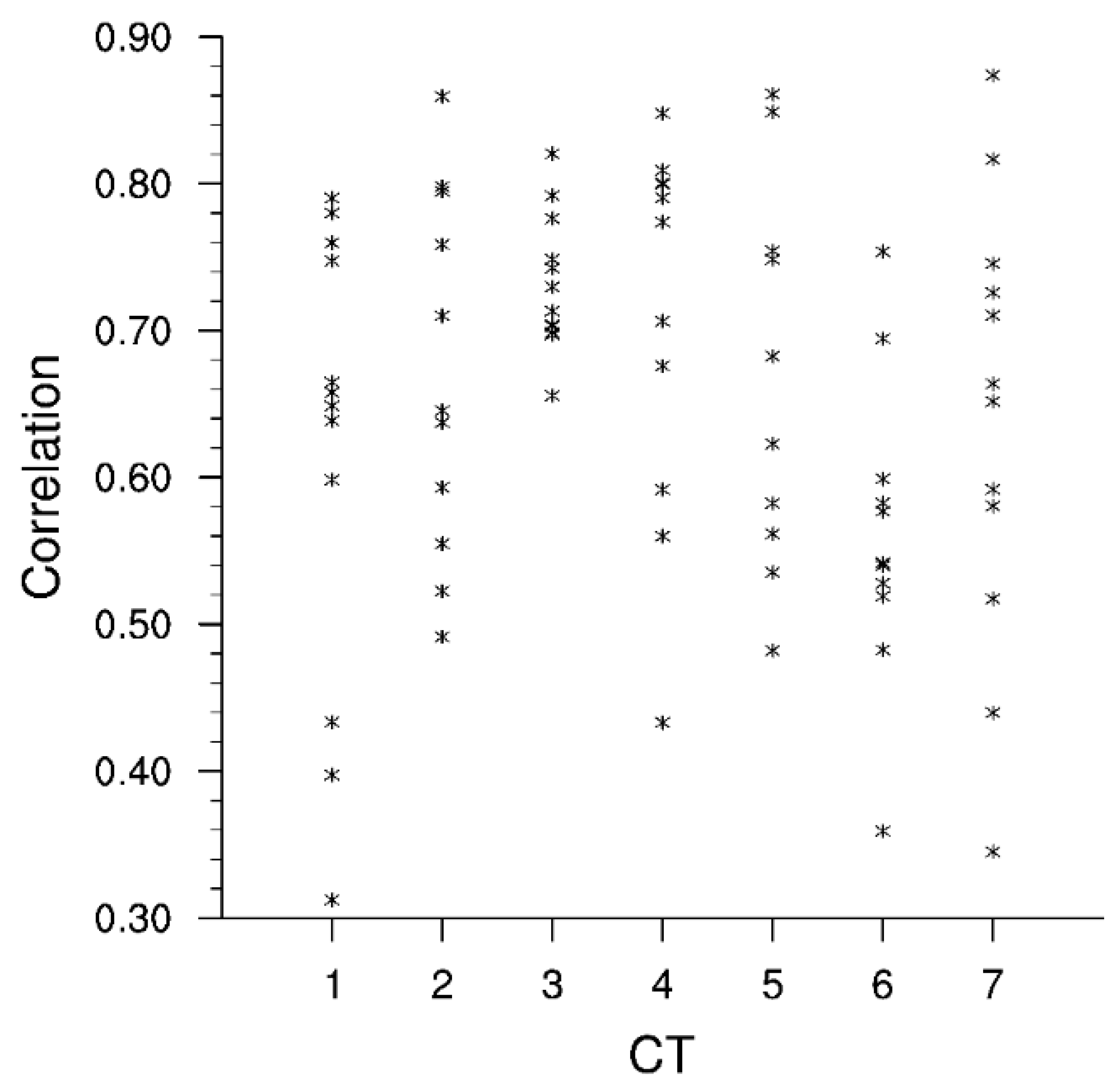
Figure 4 and Figure 5 support this approach for using the monthly representative patterns of each circulation type. Figure 4 shows the wind-field patterns of CT 1 in each month over the southern Caribbean and northwest region of South America; no two patterns are the same, and as such, each can be considered as a separate wind class. In addition, Figure 5 shows that the monthly patterns of CT 1 have a wide range of correlations (0.31–0.79) with the long-term mean pattern for CT 1. This wide range of correlations shows that the typical monthly wind-field patterns could possibly account for the high intra-cluster variability, except for CT 3, which has a narrower range of correlations, between 0.65 and 0.82. Thus, our approach for defining the wind classes as the monthly wind-field patterns for each circulation type accounts for the high intra-cluster variability within each circulation type and the influence of the seasonality on the atmospheric circulation patterns.

2.3.3. Accuracy of Eighty-Two Wind Classes Versus Seven Wind Classes in Reproducing the Long-Term Mean Wind-Field Pattern at the 10 m Level

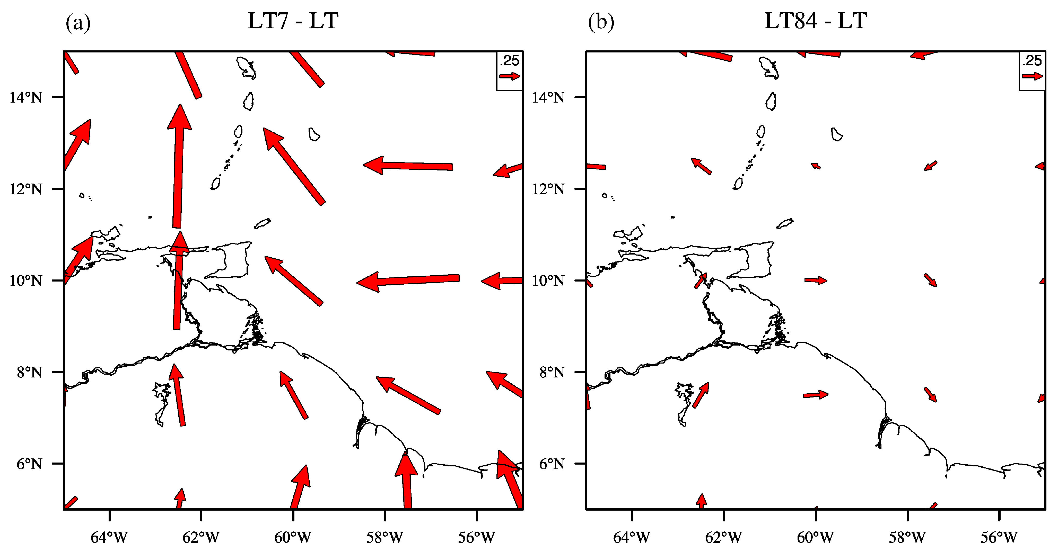
One main concern is the improvement that eighty-two wind classes could provide versus seven wind classes from the seven main circulation types. To assess this improvement, the reproduction of the long-term mean 10 m wind field was determined from both seven circulation types and eighty-two wind classes. Surface-level winds (in addition to the upper-level winds and other meteorological parameters) are taken as input to the numerical weather prediction model in the next step of the SDD process. The long-term mean wind field from seven classes (LT7) was determined by weighting the class patterns with their frequency of occurrence. This was repeated for 82 wind classes to produce the long-term mean wind field (LT82). The error was computed as a vector error between the long-term mean wind field, as derived from the wind classes, and the actual long-term mean, using the full 32-year dataset. These vector errors are shown in Figure 6. The eighty-two wind classes provide a more accurate representation of the mean large-scale 10 m wind field than just the seven typical CT patterns.
In Figure 6a, the difference between the derived long-term field created with seven wind classes (LT7) and the actual long-term mean (LT) is depicted, while in Figure 6b, the difference between the derived long-term field created with eighty-two wind classes (LT82) and the actual long-term mean is shown. The vector error in using eighty-two wind classes is smaller than that if seven wind classes were used. The sum of all the vector component differences squared for LT82—LT (Figure 6b) (150.3 m2 s−2) is smaller than that for LT7—LT (Figure 6a) (398.8 m2 s−2). As such, eighty-two wind classes provide a more accurate representation of the long-term wind fields over the Caribbean than seven wind classes. Therefore, 82 wind classes were used in the subsequent steps of the SDD method.

2.4. Downscaling the Large-Scale Wind Fields Using a Numerical Weather Prediction Model

NWP models are used to downscale large-scale weather conditions to more localized atmospheric information by incorporating the effects of the terrain and resolving finer-scale features, such as sea breezes and convective systems, and incorporating physical processes, such as turbulence. In this study, the NWP model used to adjust the large-scale atmospheric fields for mesoscale topographic conditions is the Weather Research and Forecasting (WRF) model, Advanced Research core, version 3.5.1 [53]. In the following subsections, we describe the computational setup of the WRF model by describing (i) the modeling domain, (ii) its parameterization configurations, (iii) the input surface and terrain datasets, and, finally, (iv) the input atmospheric conditions corresponding to the wind classes.

2.4.1. Modeling Domain

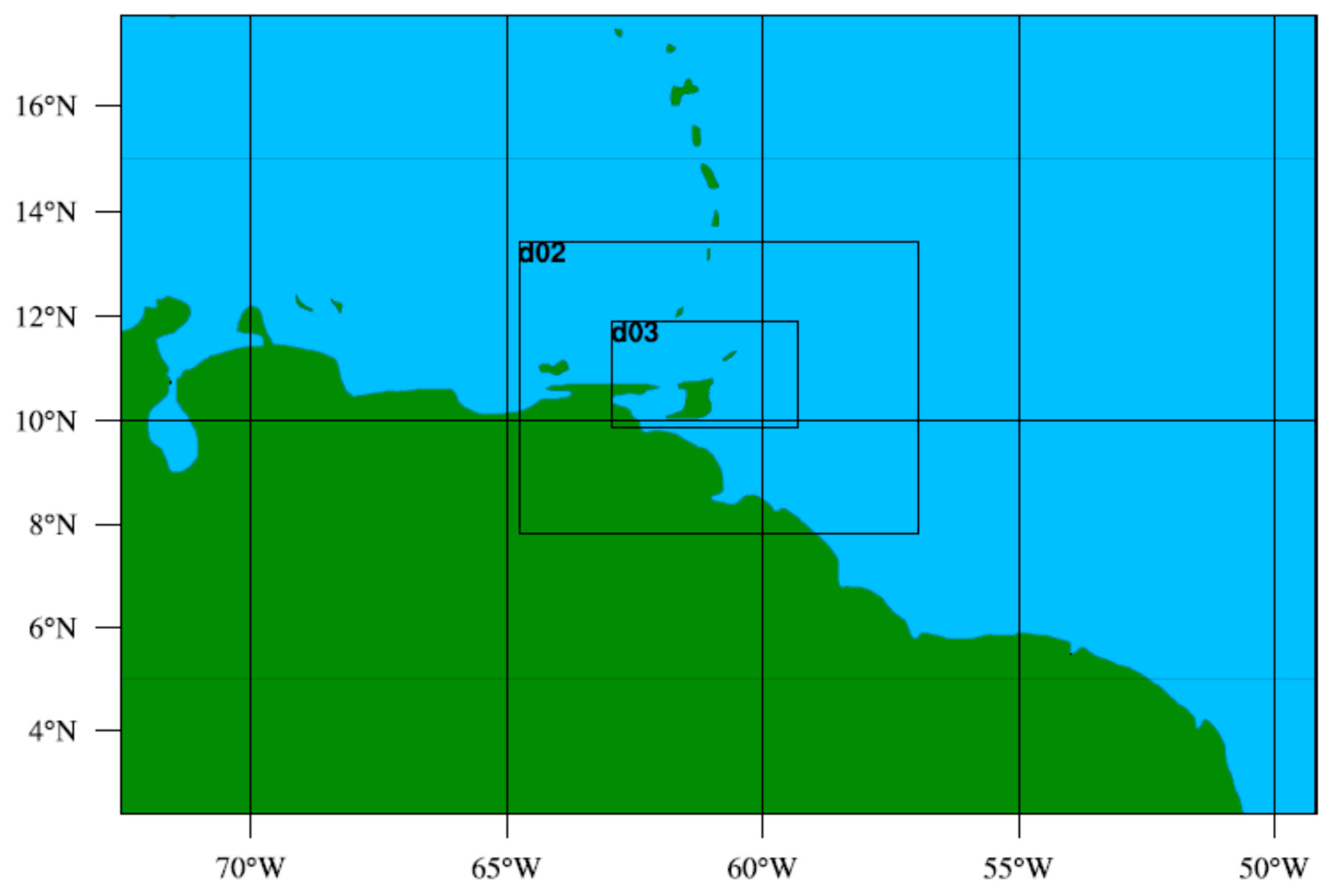
The modeling domain consisted of two telescoping nests centered at 10.69° N and 61.47° W, with a Mercator projection. The outermost domain’s (D01’s) horizontal resolution was 25 km, with the first nest having a resolution of 5 km and the innermost nest having a 1 km resolution (Figure 7). The outermost domain (d01) consisted of 91 × 61 grid points, the first nest (d02) comprised 151 × 111 grid points, and the second nest (d03) spanned 331 × 196 grid points. WRF was configured with two-way communication between the nests and the parent domain. The highest-resolution grid encompassed Trinidad and Tobago and a part of Venezuela, on the South American continent (d03). The model was configured with thirty-four vertical levels, with the first six levels above ground at approximately 14 m, 42 m, 76 m, 117 m, 191 m, and 277 m. The wind maps were produced from the outputs of the d03 domain, which is the study region.

2.4.2. WRF’s Parameterization Schemes

WRF (and other NWP models) use parameterization schemes to represent subgrid-scale atmospheric processes. These processes are smaller than the model’s grid resolution and are not resolved because of computational limitations. The key processes that are parameterized are radiation (longwave and shortwave), convection, turbulence, and cloud microphysics. The simulated wind fields are sensitive to the PBL scheme. As such, sensitivity studies were previously conducted to determine an appropriate planetary boundary layer (PBL) scheme that best represents wind speeds and their probability distributions [35]. For the case study islands, Trinidad and Tobago, the chosen PBL scheme was determined to be the Yonsei University PBL scheme with the topographic drag enabled [35]. As such, based on [35], WRF was configured using a set of physical parameterizations, as illustrated in Table 1.

2.4.3. Input Surface and Terrain Datasets

WRF’s preprocessor (WPS) generates topographical input data for WRF from land cover and terrain datasets. The WRF land cover characterization (LCC) (USGS/GLCC) at a 30-arcsecond (~900 m) resolution provided land use in 24 categories and soil in 16 categories and was used in conjunction with the USGS 30-arcsecond elevation data (GTOPO30).

2.4.4. Initial and Boundary Input Conditions for Each Wind Class

The National Center for Environmental Prediction—Department of Energy (NCEP/DOE) reanalysis provided the necessary initial and boundary conditions. Pressure-level parameters and surface parameters were provided on a grid of 2.5 ° × 2.5 ° resolution. The initial and boundary conditions (ICBCs) were determined for each of the 82 wind classes as follows: Each wind class is a monthly wind pattern for each circulation type. For the atmospheric ICBCs, the day which daily wind pattern is closest to the mean monthly wind pattern for each circulation type was chosen for the NWP simulations. The ICBCs were drawn from the NCEP/DOE reanalysis at 1200 UTC of the previous day. In this way, WRF was reinitialized from a “cold start” at 1200 UTC daily and allowed to run for 36 h, with the first 12 h taken as the spin-up period as in [35]. The spin-up period allows mesoscale information that is not present in the reanalysis data to develop. Atmospheric boundary conditions at the outermost domain were updated every 6 h by the model. No observational or grid nudging was used to adjust the simulated pressure and wind fields to the reanalysis data. As nudging prevents the simulated wind, pressure, and temperature fields from drifting away from the large-scale forcings provided by the reanalysis, the simulations in this work are short-term simulations, and reinitializations of the WRF model daily prevents excessive drift away from the reanalysis boundary conditions. In addition to atmospheric fields, sea surface temperatures (SSTs) are needed, as a substantial portion of the domain contains the Caribbean Sea and the Atlantic Ocean. SSTs contribute to the boundary conditions. Skin temperatures from the reanalysis provided the SSTs. SSTs, once initialized each day, were constant throughout the integration period.

2.4.5. Processing of the WRF’s Wind Speed Output

WRF provides the 10 m wind speeds as an output and wind components at model levels. WRF determines the 10 m wind speeds using surface layer physics, which is the Monin–Obukhov similarity theory in this study’s configuration of the model (Section 2.4.2). To determine the 50 m and 80 m wind maps, wind vector components from the seven lowest model levels of the computational grid (refer to Section 2.4.1) were fitted to a cubic spline, which was used to interpolate the wind vector components to the required heights.

2.4.6. Summary of Step 2 of the SDD Method

In Step 2 of the SDD method, the atmospheric conditions of each wind class are dynamically downscaled using the WRF model. Figure S2 shows the transformation of the wind classes to the input data to the high-resolution simulation. The 10 m wind speeds at a random grid point corresponding to the high-resolution simulations of four wind classes are shown in Figure S3. These wind classes show different diurnal variations. However, some wind classes produce similar diurnal patterns but with a difference in the timing of the maximum wind speed and with varying maximum wind speeds.

2.5. Climatological Wind Map Creation

2.5.1. Wind Speed and Wind Power Densities

The climatological wind maps were determined by weighting the high-resolution simulations with the frequency of the occurrence of the large-scale wind classes derived from the atmospheric circulation catalog. The general method by Frey-Buness et al. [36] is adopted and outlined as follows: Let { ϕ i : i = 1 K } denote the wind classes and P ϕ i be the probability that the ith pattern occurs. As the K wind classes are assumed to cover all the atmospheric states, P ϕ i is then the frequency of the ith pattern in developing the climate and
i = 1 K P ϕ i = 1 .
Now, consider the ‘local-scale’ wind speeds ( V j ) found from the high-resolution dynamical simulations. Suppose { V j :   j = 1 n } covers all the possible wind speeds occurring at each grid point, and V j is the wind speed at one of the jth hours of any 24 h simulation associated with one of the circulation patterns. Therefore, at the local scale and for each circulation type,
j = 1 n P V j = 1 .
Let P V j | ϕ i be the conditional probability that the ‘local-scale’ grid-point wind speed ( V j ) occurs if the wind class is ϕ i . Then, the probability that V j occurs is
P V j = i = 1 K P V j | ϕ i · P ϕ i .  
where P V j | ϕ i varies for each grid point.
The statistical moments for wind speed V μ , with μ indicating the order of the moments, may be estimated as follows [36]:
V μ = i = 1 K P ϕ i · V μ ϕ i  
where
V μ ϕ i = j = 1 n P V j | ϕ i · V j μ .  
Equation (4) was used to determine the mean wind speed and the wind power density (WPD) climate by estimating the first moment, which is the mean wind speed, and the third moment, which contributes to the WPD as follows:
P D ¯ = 1 2 ρ V 3
The air density at each hour of each simulation was calculated using WRF’s output of the relative humidity, air temperature, and pressure [54]. The long-term air density ( ρ ) in Equation (6), at each grid point, was determined in a similar manner as the mean wind speed in Equation (4), with ‘ V ’ replaced by ‘ ρ ’.

2.5.2. Processing High-Resolution Simulations to Create Wind Maps

Wind maps are created at several heights above ground level. In this work, we present maps for three heights for simplicity: 10 m, 50 m, and 80 m. To create these maps, the wind speeds at each grid point of the modeling domain were collated across all the wind classes. From these, the wind speed intervals and frequency of the occurrence of each wind speed interval were computed. The probabilities ( P V j | ϕ i ) were subsequently calculated from these frequencies prior to applying Equations (3)–(6). This computational procedure is depicted in Figure S4.

2.5.3. Validation of the Wind Maps at the 10 m Height

The validation is for 10 m maps, as wind data were obtained through the USA National Climatic Data Center’s website for the two sole long-term stations maintained by the Meteorological Service of Trinidad and Tobago. These two climatological stations record wind data at only 10 m above ground level (AGL) at Crown Point, Tobago (the smaller island) and Piarco, Trinidad (Table 2). Weather observations at climatological stations are collected according to World Meteorological Organization (WMO) standards [55]. Hourly wind data for the period 1 January 1989 to 31 December 2009 were used to validate the wind maps. The quality checks of the wind data are detailed in [56].
The validation of the 10 m wind maps entails (i) a comparison of the estimates of the observed long-term average wind speed and WPD with those from the wind maps, (ii) a comparison of the observed wind speed distributions and the simulated distributions, and (iii) a comparison of the variations in the annual wind speeds and WPDs between the observations and the simulated values.

2.5.4. Interannual Variability

In this study, we consider that the interannual variability in the wind resources is determined primarily by the frequency of the wind classes. Because a particular combination of frequencies determines the long-term climatological maps, the deviations of the frequencies in the wind classes in each year from this specific combination will determine the deviations from the climatological wind map. Thus, to assess the interannual variability in the wind maps, the frequencies of the wind classes in each year were compared with their long-term frequencies by dividing them by their corresponding long-term frequencies. These weighted frequencies ( W y r ϕ i ) were used in Equation (4) in the replacement of P ϕ i . The mean wind speed in each year was then determined by normalizing the right-hand side of Equation (4) by the sum of the weighted frequencies via
V μ y r = i = 1 K W y r ϕ i · V μ ϕ i i = 1 K W y r ϕ i .

3. Results and Discussion

3.1. The Validation of the 10 m Wind Maps

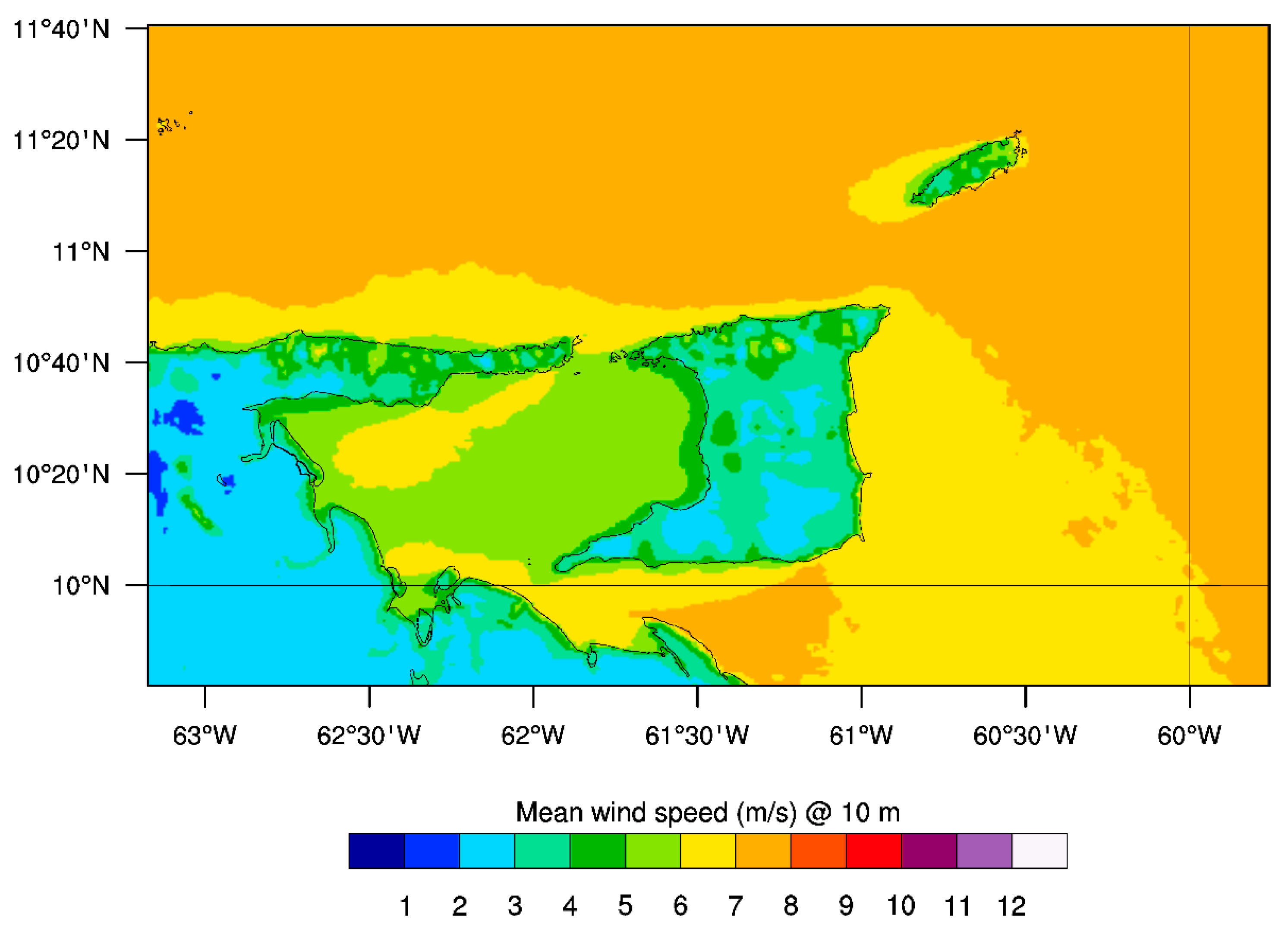
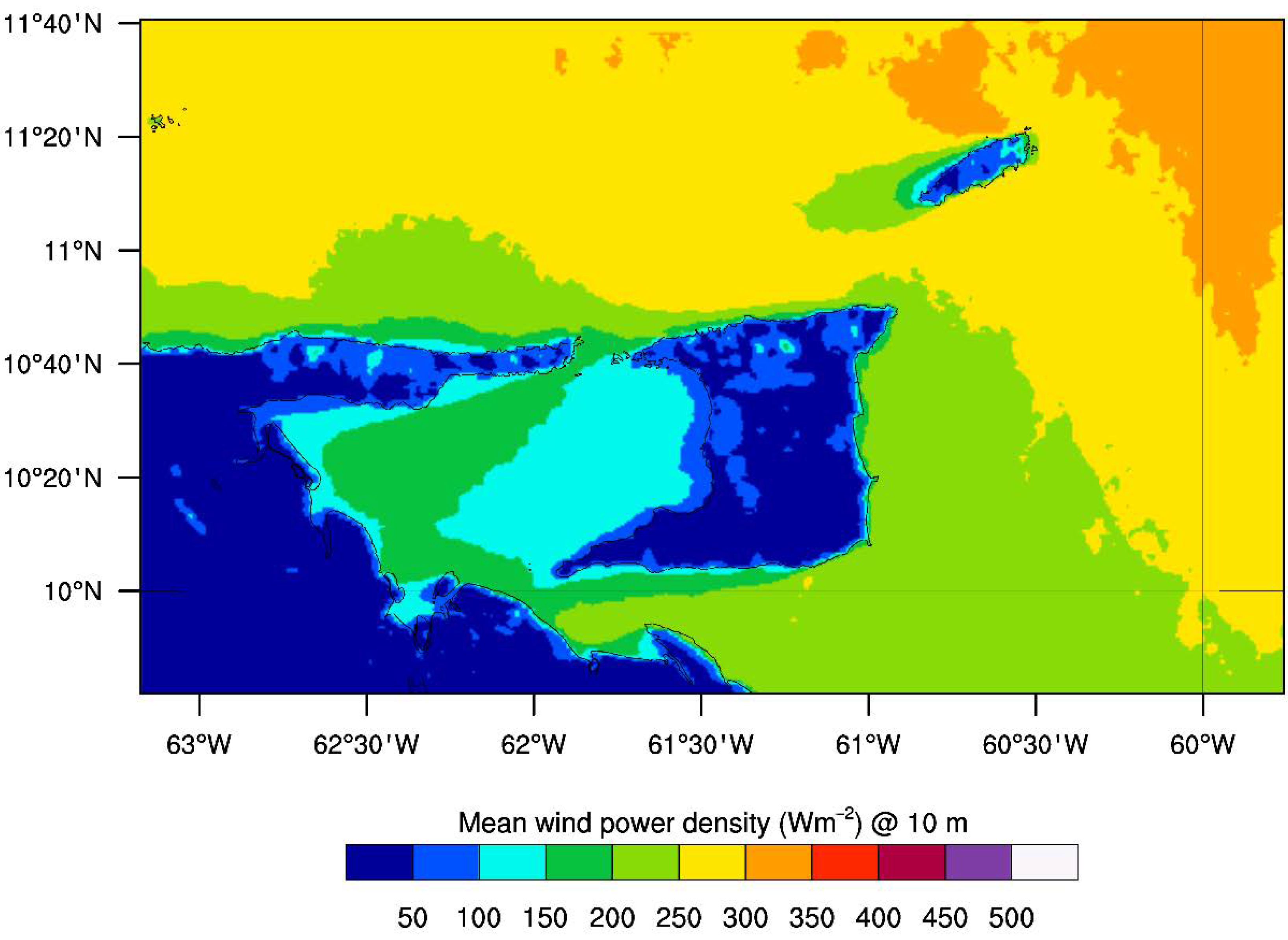
The 10 m wind speed and wind power density (WPD) maps for Trinidad and Tobago were validated using climatological averages from existing in situ wind data. The 10 m wind speed and WPD maps for Trinidad and Tobago are shown in Figure 8 and Figure 9. At the 10 m level, in both Trinidad and Tobago, the wind speeds vary from 2 to 6 m s−1, and the WPDs are lower than 100 W m−2 in most areas on the two islands.
The comparisons of the simulated wind speeds and the observed wind speeds at the meteorological stations show relatively good agreement at the 10 m level. The in situ mean wind speeds at these sites were 3.56 m/s and 2.92 m/s, respectively [56]. The corresponding simulated long-term mean wind speeds from the 10 m wind map were taken as the wind speeds from the closest grid point to each station (Table 2). These were 4.02 m/s and 3.52 m/s at Crown Point and Piarco, respectively, resulting in a bias of +0.46 m/s and approximately 15% higher than the actual mean wind speed for Crown Point and +0.60 m/s, or about 18% higher than the mean wind speed, for Piarco. These positive biases show a tendency for the wind speeds to be overpredicted at the two low-lying measurement stations. The mean bias of +0.53 m/s, calculated herein, is only representative of low elevations and at the 10 m height. For these reasons, as well as that bias could vary with height, we do not correct the 50 m and 80 m wind maps (Section 3.2) for bias. Furthermore, at greater heights, where the wind speeds are more moderate, the bias could be smaller, as the NWP model configuration is known to not capture low wind speeds adequately [35]. In addition, some bias is expected, as differences exist between the model’s grid cell surface characteristics (e.g., mean elevation) and those at the measurement stations, and the bias obtained in this study is comparable with those obtained in other regions, such as the eastern Mediterranean Basin [30]. The simulated wind speed probability density distributions, when weighted, produced wind power densities (WPDs) of 63.4 W m−2 at Crown Point and 54.3 W m−2 at Piarco and a difference of 9.4–12.9 W m−2 (an average of 11.2 W m−2) compared to the corresponding actual WPDs of 56.0 W m−2 and 41.4 W m−2.
In addition, the wind speeds and wind power densities at Crown Point and Piarco were determined from the Global Wind Atlas (GWA) [21] for comparison. At Crown Point, the GWA’s wind speed and WPD are 4.71 m s−1 and 88 W m−2, respectively. These are higher than the corresponding values of the SDD method by 0.69 m s−1 and 24 W m−2, respectively. The GWA overestimates the average wind speed and WPD at Crown Point by 1.12 m s−1 and 32 W m−2, respectively. At Piarco, the GWA’s wind speed and WPD are 3.34 m s−1 and 31 W m−2, which are lower than those of the SDD method herein by 0.18 m s−1 and 10 W m−2. The GWA overestimates the average wind speed at Piarco by 0.42 m s−1 and underestimates the WPD by 10 W m−2. The GWA’s average wind speed bias is thus 0.77 m s−1, and the bias for WPD is 11 W m−2. The average wind speed bias is slightly higher than that for the SDD method, and the bias for WPD is the same. The SDD method performs slightly better for the two stations on an average basis.
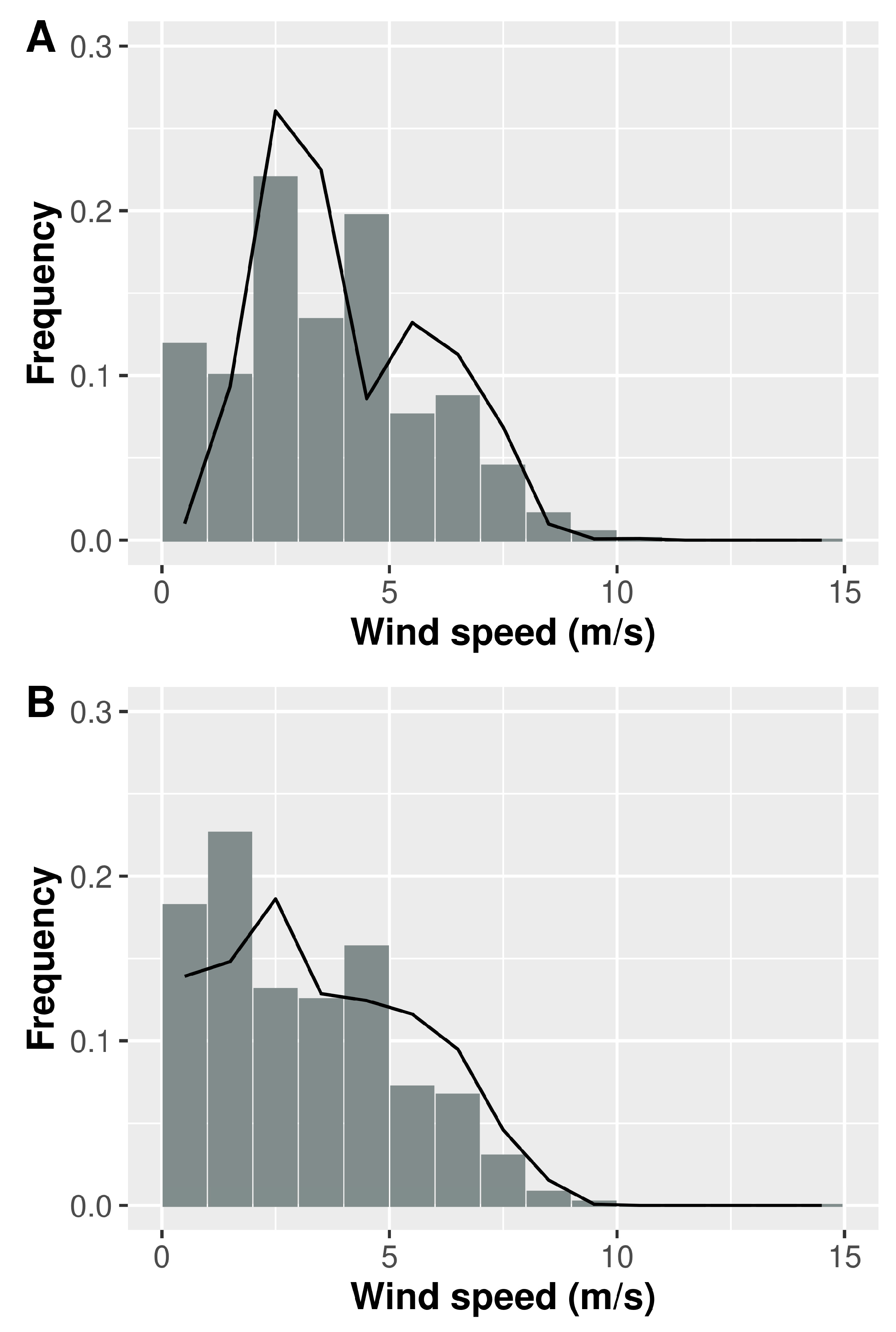
Figure 10 shows the simulated wind speed distributions at Crown Point and Piarco. Compared with the long-term histograms [56], we find that the frequencies of low wind speeds, those lower than 2 m/s, are underpredicted at both sites, while the frequencies of the 2–3 m/s and 3–4 m/s wind speed intervals are overpredicted. However, the total frequency up to the 4 m/s wind speed bin is captured by the simulations, with approximately 57% from simulations versus 59% from observations at Crown Point and 60% low wind speeds from simulations versus 66% from observations at Piarco. In addition, the SDD method captures a higher frequency of low wind speeds (<4 m/s) at Piarco than at Crown Point.
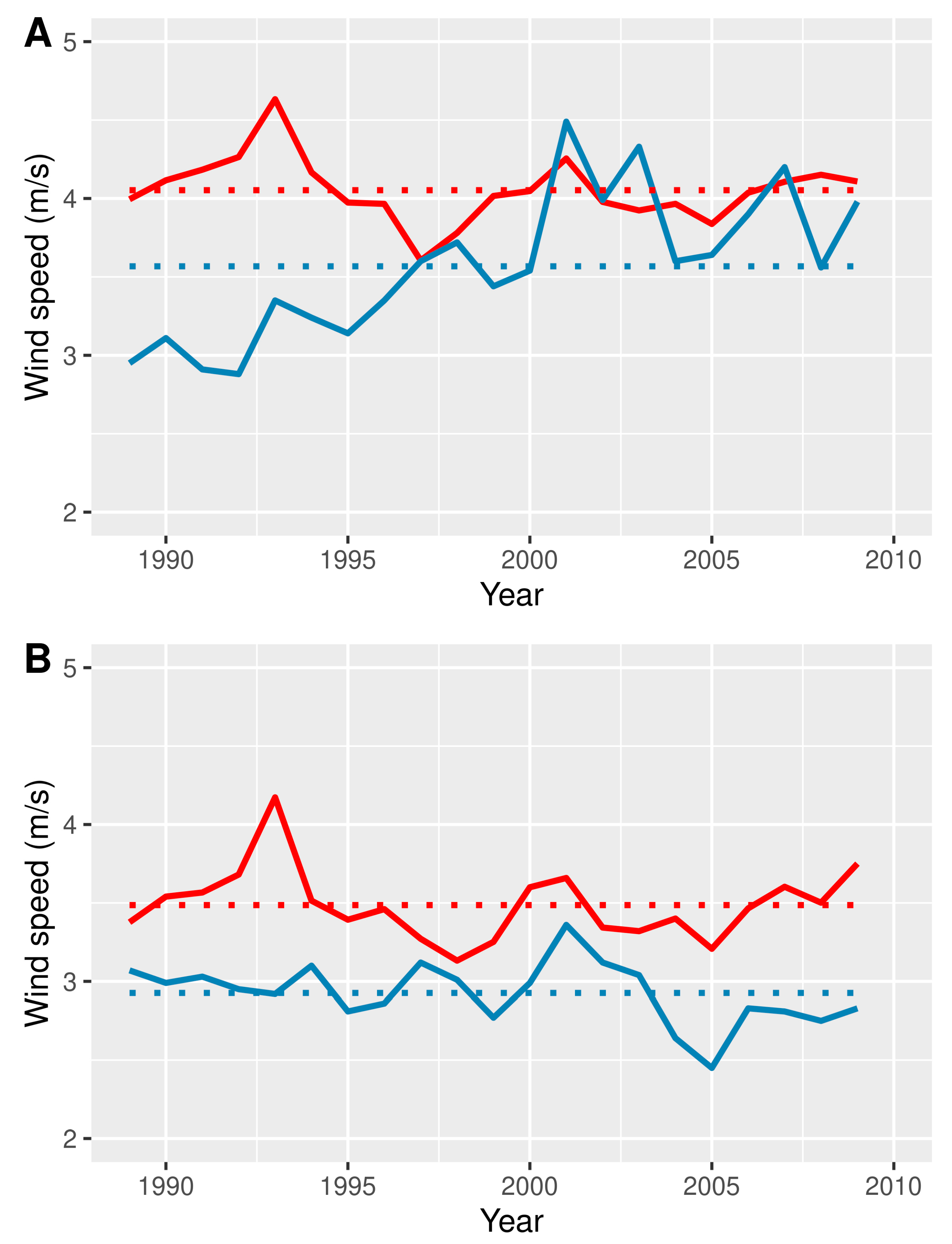
Another measure of the performance of the proposed statistical–dynamical downscaling scheme for wind map generation is its ability to simulate the interannual variability in wind speeds (Figure 11 and Table 3). The statistical–dynamical method using atmospheric circulation patterns accounts for a high degree of the interannual variability in the wind. The interannual variation, when quantified as a percentage deviation from the long-term mean, is from −11.6% to 13.6% at Crown Point and from −10.7% to 18.9% at Piarco. The interannual variation at Piarco is similar to that shown by the in situ data. The upper bound of 18.9% is higher than that shown by the in situ data, which is expected, as wind speeds at the 10 m level are overestimated. The lower bound of the interannual variation (−10.7%) at Piarco is smaller in magnitude than that shown by the in situ data (−16.3%). Again, this may be because of the overestimation of wind speeds at the 10 m level and the WRF model’s (or any NWP model’s) ability to capture low wind speeds. The simulated annual wind speeds at Piarco are like the in situ data’s annual variation in wind speeds. Although the simulated interannual variability at Piarco, ±18.9%, is similar to that exhibited by the in situ data (±16.3%), the simulated interannual variation at Crown Point (±13.6%) is almost half that shown by the in situ data (±25.9%). This difference between the simulated and in situ variations may be because of the model not capturing a possible increasing trend in the wind speed at Crown Point. An investigation into possible trends at Crown Point would require rigorous statistical analyses to confirm whether an increasing trend exists and whether other factors are affecting the microclimate at Crown Point.
It is expected that any statistical–dynamical downscaling method may not be able to explain all the interannual variation, as the class generation scheme for the empirical probability density function of the wind speed is only based on the classification of the large-scale atmospheric circulation using wind components, the main large-scale factor affecting winds at the near-surface level. It is possible that 82 wind classes may not be sufficient to describe atmospheric conditions contributing to very low-wind years or very high-wind years or the input reanalysis dataset does not capture the full impact of the interannual variability on local-scale winds. A previous study [35] investigated the choice of input reanalysis data by assessing their ability to minimize the spatial error in simulated wind speeds. However, the comparison of the interannual variation in this study indicates a necessity to check whether the input reanalysis data can capture the interannual variation in measured data. Nevertheless, the proposed method appears to capture a significant portion of the interannual variation, at least at sites with no discernible increasing or decreasing trends in wind speed.

3.2. The 50 m and 80 m Wind Maps for Trinidad and Tobago

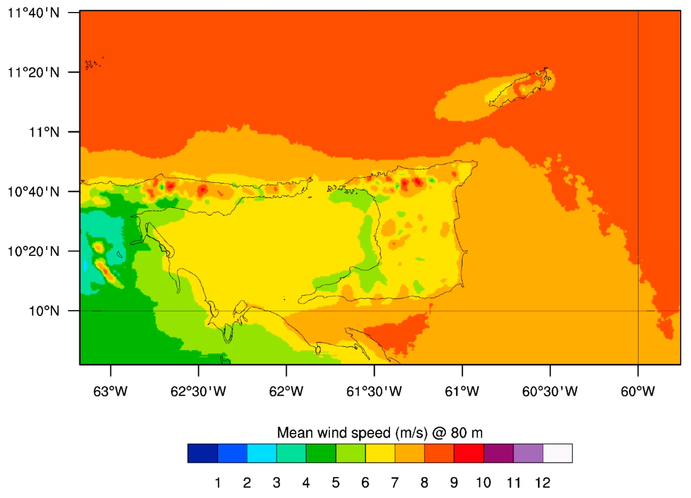
The wind speed maps for Trinidad and Tobago, at 50 m and 80 m heights, are shown in Figure 12 and Figure 13, respectively. An average wind speed of 6–7 m s−1 at the hub height is generally considered as the threshold for economically feasible wind farm developments [57]. The wind maps show a good wind regime (>6 m/s) along the Northern Range; the north, east, and south coasts of Trinidad; in the central area of west Trinidad; and in most of Tobago at 50 m, with an excellent offshore wind resource. The wind regime in other areas is generally low. However, the majority of the two islands has good to moderate resources at 80 m, which is a promising result in that land space for wind farms may not be available when constraints, such as population density and environmentally sensitive areas, are applied. Suitable inland areas for further exploration are hilly areas and the coastlines exposed to the prevailing winds, as well as areas in central Trinidad, which were previously not known to have moderate wind resources. In addition, for offshore wind, the 50 m height, and taller, gives wind speeds faster than 7 m s−1. The offshore areas to the north, east, and south of Trinidad warrant further investigation.
The wind power density maps are shown in Figures S5 and S6 for the 50 m and 80 m heights, respectively. The 50 m WPD map shows that WPDs are generally lower than 200 W m−2 across Trinidad and Tobago, except for two areas in the northern range of Trinidad and two areas in the central and northeast of Tobago, where WPDs are 350–400 W m−2. At the 80 m height, the WPDs of most areas on land in Trinidad are lower than 250 W m−2, while those of most areas on land in Tobago are higher than 250 W m−2. In addition, the 80 m WPD maps show that the offshore area between Trinidad and Tobago are of higher wind potential (350–400 W m−2). The WPD maps confirm the areas that could be prioritized from the wind speed maps. However, the 80 m WPD map also enhances the possibility of the offshore region between the islands for offshore wind farm developments.
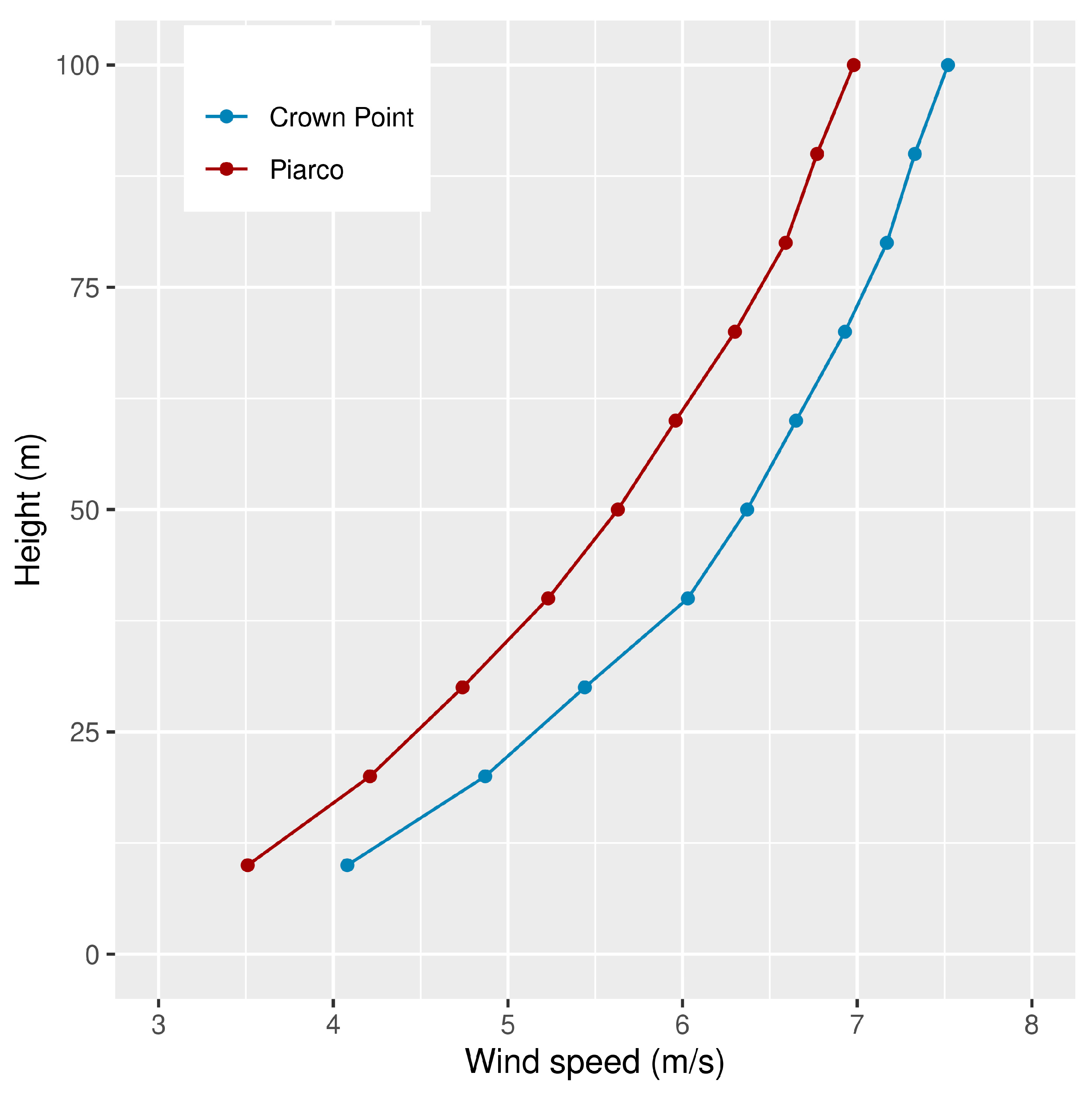
The variations in the wind speeds in the vertical direction at the two climatological stations are shown in Figure 14. These follow an approximate power law relationship with height. The wind shear exponents for wind speeds between 50 m and 10 m, 100 m and 10 m, and 100 m and 50 m are given in Table 4. The shear exponents at Crown Point are approximately two times the traditionally used 1/7 power exponent and are comparable to the mean monthly shear exponents, which were estimated from extrapolating the 10 m Weibull shape and scale parameters in a previous study [55] for both Crown Point (from 0.229 to 0.259) and Piarco (from 0.249 to 0.282). The shear exponents from the NWP in this study are still higher than the estimated exponents. The shear exponents for Crown Point are expected to be lower than those for Piarco, as Crown Point is a coastal site that is better exposed to the prevailing winds. Crown Point’s lower exponents mean that wind speeds of a specific value will be attained at a lower height at Crown Point than at Piarco. For example, from Figure 14, wind speeds at Crown Point attain a value of 7 m s−1 at approximately 75 m AGL, while at Piarco, the same wind speed is attained at approximately 100 m AGL. Crown Point has the advantage of stronger winds than Piarco at the 10 m level because of exposure to higher wind speeds from over the ocean.
In addition, the vertical wind speeds at the 50 m level were compared with those from the GWA: 5.59 m s−1 for Crown Point and 4.74 m s−1 for Piarco. The corresponding values from the SDD method are 6.19 m s−1 and 5.83 m s−1, respectively. The SDD method predicts higher average wind speeds than the GWA by 0.60 m s−1 and 1.09 m s−1, respectively. The absence of measurements at heights greater than 10 m AGL prevents further comparisons.

3.3. Implications

3.3.1. Small-Scale Wind Power

As Trinidad and Tobago is an energy-intensive island state, the suitability of wind power for its electricity needs must be considered. First, the wind maps were evaluated for small-scale and utility-scale wind power. Because of its location in the tropics, the island state has lower average wind speeds compared with those in temperate regions, as observed from the global wind maps [21]. At the 10 m level, wind speeds are lower than 6 m s−1, and low wind speeds are prevalent (~60% lower than 4 m s−1), thereby limiting small-scale wind power. From the 10 m wind maps, thin coastline strips around Tobago and on the northern, southern, and eastern coasts of Trinidad appear to be useful for small-scale wind power applications, as the average wind speed is higher than 5 m s−1. These coastline strips are also used for tourism activities. The next steps should consider the economic and financial feasibility of small-scale wind turbines in offsetting electricity needs in the tourism industry. Additionally, the testing of wind turbines under corrosive coastal conditions is essential in understanding their durability and, therefore, their lifetime for tourism needs.

3.3.2. Utility-Scale Wind Power

For large-scale onshore wind power, all of Tobago and most of Trinidad can be considered as promising for large-scale wind power onshore at the 80 m height, while the 50 m height is the minimum height for offshore wind turbines. In addition, the offshore area between the two islands is highlighted by the 80 m wind map as a possibility for offshore wind farm development. A detailed wind resource assessment campaign using meteorological towers, SODARS, and LIDARS would enable the bias correction of higher-level wind maps. Validated wind maps, a wind resource measurement campaign for bankable onsite measurements of potential wind farms, and site layout studies are needed prior to economic and financial studies for proper decision making in charting the developments of onshore and offshore wind power in the island state.

3.3.3. Backup Energy Storage

In addition, improving the estimates of the interannual variability is important for the financial modeling of future wind farms to determine the financial reserves needed for low-wind years. Furthermore, the analysis of the interannual variation at one site indicates a microclimate with significant interannual variation and possibly a trend (Figure 11A). As such, it would be beneficial to ensure long-term wind measurements are taken at sites earmarked for wind farm developments.
The wind maps produced provide long-term wind speed and wind power density averages. However, the wind is known to fluctuate at hourly and sub-hourly scales. Ongoing wind measurements and an assessment of the historical sub-hourly fluctuations would assist in determining the quantities of backup energy storage methods, such as fossil fuel plants and battery energy storage systems (BESS). In addition, further studies should assess and determine appropriate prediction models for extended daily wind droughts, hourly wind ramps, and hourly or daily extreme wind events, as these types of events would determine the size of the backup energy resources.

3.3.4. Higher-Resolution Modeling and Climate Impact Studies

It would be interesting to repeat this study at even higher resolutions for the NWP simulations. The current study was limited by the resolution of the input topographic datasets to the NWP model. However, increased resolutions in the topographic dataset could assist with investigating whether a higher resolution, say 200 m × 200 m, would provide a better assessment of the wind resources, and if so, what aspects of mesoscale features, such as sea and land breezes, would be better resolved.
Furthermore, an assessment of the potential changes in the future wind climate would determine sites that would benefit from an increase in wind power or whether sites might potentially undergo a decrease in wind power. The SDD method in this study can be used in efficiently downscaling climate change data over the next 75 years or longer to make such assessments. The wind maps created in this study can serve as baseline maps for such climate change impact assessment studies.

4. Conclusions

In this work, a statistical–dynamical downscaling technique with 82 wind classes derived from typical atmospheric circulation patterns based on wind fields and the WRF numerical weather prediction model was proposed to develop high-resolution wind maps. This approach was applied to the Caribbean region to determine wind maps for the small island state of Trinidad and Tobago.
At the 10 m level in both Trinidad and Tobago, the wind speeds vary from 2 to 6 m s−1, and WPDs are lower than 100 W m−2 in most areas. The 10 m wind maps were validated with the mean wind speed data from the two sole meteorological stations and showed good agreement with the data. These 10 m wind maps are the first set of validated wind maps for Trinidad and Tobago. At the 10 m level, the model data show a +0.5 m/s bias. Validation of the wind maps at other heights will be possible as more extensive datasets with measurements at several heights become available.
The wind maps developed in this study offer a significant benefit in determining areas that could be given priority in finding locations for monitoring wind resources. The 80 m wind map developed indicates that the islands have from good to moderate wind resources (>6–7 m s−1) and that this is the minimum height to be considered for wind turbine hub heights in utility-scale power applications. For offshore considerations, the 50 m height and higher might be suitable for power applications. Future studies should analyze the economics of utility-scale wind power. These wind maps can help to identify priority areas and the minimum heights for detailed wind measurements in Trinidad and Tobago. The 80 m height is preferred on land, as this height allows for more areas to be considered for wind farm developments, especially when environmentally sensitive areas might have to be considered.

Supplementary Materials

The following supporting information can be downloaded at https://www.mdpi.com/article/10.3390/wind5010007/s1, Figure S1: Data flow and processing stages for Step 1 of the SDD method; Figure S2: Transformation of the wind classes to the input data to the high-resolution simulation by downscaling via the WRF NWP in Step 2; Figure S3: The 10 m wind speeds at a random grid point in the d03 domain corresponding to the high-resolution simulations of four wind classes; Figure S4: Transformation of the high-resolution wind speeds to maps of wind speeds and wind power densities in Step 3; Figure S5: Wind power density at 50 m AGL in and around Trinidad and Tobago; Figure S6: Wind power density at 80 m AGL in and around Trinidad and Tobago.

Author Contributions

Conceptualization, X.T.C. and N.R.S.; methodology, X.T.C.; software, X.T.C. and N.R.S.; validation, X.T.C.; formal analysis, X.T.C. and R.M.C.; investigation, X.T.C., N.R.S. and R.M.C.; resources, N.R.S. and R.M.C.; data curation, X.T.C. and N.R.S.; writing—original draft preparation, X.T.C.; writing—review and editing, X.T.C., N.R.S. and R.M.C.; visualization, X.T.C.; supervision, R.M.C.; project administration, X.T.C. and N.R.S. All authors have read and agreed to the published version of the manuscript.

Funding

This research received no external funding.

Institutional Review Board Statement

Not applicable.

Informed Consent Statement

Not applicable.

Data Availability Statement

The NCEP-DOE Reanalysis 2 data were provided by the NOAA/OAR/ESRL PSD, Boulder, Colorado, USA, from their Web site at http://www.esrl.noaa.gov/psd/ and the meteorological data were accessed from the US National Climatic Data Center (NCDC) in 2013. The NCDC archive is available from the Climate Data Online web portal of the US’ National Centers for Environmental Information at https://www.ncei.noaa.gov/cdo-web/. The data generated are available on request from the first author.

Acknowledgments

Computational resources were provided by the Department of Physics and the Department of Computing and Information Technology at the University of the West Indies, St. Augustine Campus, Trinidad and Tobago.

Conflicts of Interest

The authors declare no conflicts of interest.

Abbreviations

The following abbreviations are used in this manuscript:
BESSbattery energy storage system
CTcirculation type
EOFempirical orthogonal function
GWAGlobal Wind Atlas
ICBCsinitial and boundary conditions
IEAInternational Energy Agency
IRENAInternational Renewable Energy Agency
LCCland cover characterization
LIDARLight detection and ranging
NCEP-DOENational Center for Environmental Prediction/Department of Energy
NWPnumerical weather prediction
PBLplanetary boundary layer
SDDstatistical–dynamical downscaling
SDGsustainable development goal
SIDSsmall island developing states
SODARsound detection and ranging
SSTsea surface temperature
UNUnited Nations
WMOWorld Meteorological Organization
WPDwind power density
WPSWRF’s preprocessor
WRFWeather Research and Forecasting

References

  1. Global Wind Energy Council (GWEC). Global Wind Report 2024. 2024. Available online: https://www.gwec.net/reports (accessed on 19 February 2025).
  2. IRENA. World Energy Transitions Outlook: 1.5 °C Pathway; International Renewable Energy Agency: Abu Dhabi, United Arab Emirates, 2021; Available online: https://www.irena.org/Publications/2021/Jun/World-Energy-Transitions-Outlook (accessed on 20 November 2022).
  3. IEA. Net Zero by 2050: A Roadmap for the Global Energy Sector; IEA: Paris, France, 2021; Available online: https://www.iea.org/reports/net-zero-by-2050 (accessed on 22 November 2021).
  4. United Nations. The 17 Goals. Available online: https://sdgs.un.org/goals (accessed on 3 April 2024).
  5. Nor, K.M.; Shaaban, M.; Rahman, H.A. Feasibility assessment of wind energy resources in Malaysia based on NWP models. Renew. Energy 2014, 62, 147–154. [Google Scholar] [CrossRef]
  6. Carvalho, D.; Rocha, A.; Gómez-Gesteira, M.; Silva Santos, C. WRF wind simulation and wind energy production estimates forces by different reanalyses: Comparison with observed data for Portugal. Appl. Energy 2014, 117, 116–126. [Google Scholar] [CrossRef]
  7. Potter, C.W.; Lew, D.; McCaa, J.; Cheng, S.; Eichelberger, S.; Grimit, E. Creating the dataset for the Western Wind and Solar Integration Study (U.S.A.). Wind Eng. 2008, 32, 325–338. [Google Scholar] [CrossRef]
  8. Yim, S.H.L.; Fung, J.C.H.; Lau, A.K.H.; Kot, S.C. Developing a high resolution wind map for a complex terrain with a coupled MM5/CALMET system. J. Geophys. Res. 2007, 112, D05106. [Google Scholar] [CrossRef]
  9. Dvorak, M.J.; Archer, C.L.; Jacobson, M.Z. California offshore wind energy potential. Renew. Energy 2010, 35, 1244–1255. [Google Scholar] [CrossRef]
  10. Larsén, X.G.; Mann, J.; Berg, J.; Göttel, H.; Jacob, D. Wind climate from the regional climate model REMO. Wind Energy 2010, 13, 279–296. [Google Scholar] [CrossRef]
  11. Frank, H.P.; Rathmann, O.; Mortensen, N.G.; Landberg, L. The Numerical Wind Atlas—The KAMM/WasP Method; Report Risø-R-1252(EN); Risø National Laboratory: Roskilde, Denmark, 2001; Available online: https://orbit.dtu.dk/en/publications/the-numerical-wind-atlas-the-kammwasp-method-2 (accessed on 27 November 2022).
  12. Nygaard, I.; Rasmussen, K.; Badger, J.; Nielsen, T.T.; Hansen, L.B.; Stisen, S.; Larsen, S.; Mariko, A.; Togola, I. Using modelling, satellite images and existing global datasets for rapid preliminary assessments of renewable energy resources: The Case of Mali. Renew. Sustain. Energy Rev. 2010, 14, 2359–2371. [Google Scholar] [CrossRef]
  13. Mortensen, N.G.; Hansen, J.C.; Badger, J.; Jørgensen, B.H.; Hasager, C.B.; Paulsen, U.S.; Hansen, O.F.; Enevoldsen, K.; Youssef, L.G.; Said, U.S.; et al. Wind Atlas for Egypt: Measurements, micro- and mesoscale modelling. In Proceedings of the 2006 European Wind Energy Conference and Exhibition, Athens, Greece, 27 February–2 March 2006; EWEA: Brussels, Belgium, 2006. [Google Scholar]
  14. Charabi, Y.; Al-Yahyai, S.; Gastli, A. Evaluation of NWP performance for wind energy resource assessment in Oman. Renew. Sustain. Energy Rev. 2011, 15, 1545–1555. [Google Scholar] [CrossRef]
  15. Kotroni, V.; Lagouvardos, K.; Lykoudis, S. High-resolution model-based wind atlas for Greece. Renew. Sustain. Energy Rev. 2014, 30, 479–489. [Google Scholar] [CrossRef]
  16. Yu, W.; Benoit, R.; Girard, C.; Glazer, A.; Lemarquis, D.; Salmon, J.R.; Pinard, J.-P. Wind Energy Simulation Toolkit (WEST): A wind mapping system for use by the wind-energy industry. Wind Eng. 2006, 30, 15–33. [Google Scholar] [CrossRef]
  17. Schwartz, M.; Elliott, D. Validation of Updated State Wind Resource Maps for the United States; NREL/CP-500-36200; National Renewable Energy Lab: Golden, CO, USA, 2004. Available online: http://www.nrel.gov/docs/fy04osti/36200.pdf (accessed on 20 November 2022).
  18. Alonso, Y.; Martinez, Y.; Roque, A.; Yu, W.; Borrajero, I. A post-processing module based on Cressman’s analysis to improve the Wind Energy Simulation Toolkit mapping system. Wind Eng. 2019, 43, 277–298. [Google Scholar] [CrossRef]
  19. Badger, J.; Frank, H.; Hahmann, A.N.; Giebel, G. Wind-climate estimation based on mesocale and microscale modeling: Statistical-dynamical downscaling for wind energy applications. J. Appl. Meteorol. Climatol. 2014, 53, 1901–1919. [Google Scholar] [CrossRef]
  20. Prieto-Herráez, D.; Frías-Paredes, L.; Cascón, J.M.; Lagüela-López, S.; Gastón-Romeo, M.; Asensio-Sevilla, M.I.; Martín-Nieto, I.; Fernandes-Correia, P.M.; Laiz-Alonso, P.; Carrasco-Díaz, O.F.; et al. Local wind speed forecasting based on WRF-HDWind coupling. Atmos. Res. 2021, 248, 105219. [Google Scholar] [CrossRef]
  21. Badger, J.; Bauwens, I.; Casso, P.; Davis, N.; Hahmann, A.; Hansen, S.B.K.; Hansen, B.O.; Heathfield, D.; Knight, O.J.; Lacave, O.; et al. The Global Wind Atlas: Introduction (Version 3.0). Available online: https://globalwindatlas.info/en/about/introduction (accessed on 5 May 2024).
  22. Le Roy, B.; Lemonsu, A.; Schoetter, R. A statistical-dynamical downscaling methodology for the urban heat island applied to the EURO-CORDEX ensemble. Clim. Dyn. 2021, 56, 2487–2508. [Google Scholar] [CrossRef]
  23. Schoetter, R.; Hidalgo, J.; Jougla, R.; Masson, V.; Rega, M.; Pergaud, J. A statistical-dynamical downscaling for the urban heat island and building energy consumption—Analysis of its uncertainties. J. Appl. Meteorol. Climatol. 2020, 59, 859–993. [Google Scholar] [CrossRef]
  24. Schubert, D.; van der Linden, R.; Reyers, M.; Fink, A.H.; Massmeyer, K.; Pinto, J.G. Statistical-dynamical downscaling of precipitation for Vietnam: Methodology and evaluation for the recent climate. Int. J. Climatol. 2017, 37, 4211–4228. [Google Scholar] [CrossRef]
  25. Chávez-Arroyo, R.; Lozano-Galiana, S.; Sanz-Rodrigo, J.; Probst, O. On the application of principal component analysis for accurate statistical-dynamical downscaling of wind fields. Energy Procedia 2013, 40, 67–76. [Google Scholar] [CrossRef]
  26. Martinez, Y.; Yu, W.; Lin, H. A new statistical-dynamical downscaling procedure based on EOF analysis for regional time series generation. J. Appl. Meteorol. Climatol. 2013, 52, 935–952. [Google Scholar] [CrossRef]
  27. Barry, R.G.; Chorley, R.J. Atmosphere, Weather and Climate, 9th ed.; Routledge: London, UK, 2010. [Google Scholar]
  28. Danzer, J.; Pieler, M.; Kirchengast, G. Closing the gap in the tropics: The added value of radio-occultation data for wind field monitoring across the Equator. Atmos. Meas. Tech. 2024, 17, 4979–4995. [Google Scholar] [CrossRef]
  29. Chadee, X.T.; Clarke, R.M. Daily near-surface large-scale atmospheric circulation patterns over the wider Caribbean. Clim. Dyn. 2015, 44, 2927–2946. [Google Scholar] [CrossRef]
  30. Hadjipetrou, S.; Kyriakidis, P. High-resolution wind speed estimates for the Eastern Mediterranean Basin: A statistical comparison against coastal meteorological observations. Wind 2024, 4, 311–341. [Google Scholar] [CrossRef]
  31. Kozyrakis, G.V.; Condaxakis, C.; Parasyris, A.; Kampanis, N.A. Wind resource assessment over the Hellenic Seas using dynamical downscaling techniques and meteorological station observations. Energies 2023, 16, 5965. [Google Scholar] [CrossRef]
  32. Xu, D.; Xue, F.; Wu, Y.; Li, Y.; Liu, W.; Xu, C.; Sun, J. Analysis of wind resource characteristics in the Ulanqab wind power base (wind farm): Mesoscale modeling approach. Energies 2024, 17, 3540. [Google Scholar] [CrossRef]
  33. Placide, G.; Lollchund, M.R. An evaluation of the reliability of the Weather Research Forecasting (WRF) model in predicting wind data: A case study of Burundi. BMC Environ. Sci. 2024, 1, 2. [Google Scholar] [CrossRef]
  34. Sperati, S.; Alessandrini, S.; D’Amico, F.; Cheng, W.; Rozoff, C.M.; Bonanno, R.; Lacavalla, M.; Aiello, M.; Airoldi, D.; Amaranto, A.; et al. A new wind atlas to support the expansion of the Italian wind power fleet. Wind Energy 2024, 27, 298–316. [Google Scholar] [CrossRef]
  35. Chadee, X.T.; Seegobin, N.R.; Clarke, R.M. Optimizing the Weather Research and Forecasting (WRF) model for mapping the near-surface wind resources over the southernmost Caribbean islands of Trinidad and Tobago. Energies 2017, 7, 931. [Google Scholar] [CrossRef]
  36. Frey-Buness, F.; Heimann, D.; Sausen, R. A statistical-dynamical downscaling procedure for global climate simulations. Theor. Appl. Climatol. 1995, 50, 117–131. [Google Scholar] [CrossRef]
  37. Commonwealth Chamber of Commerce. Trinidad and Tobago. Available online: https://commonwealthchamber.com/member-countries/trinidad-and-tobago/ (accessed on 31 January 2025).
  38. UNESCO. Tobago Main Ridge Forest Reserve. Available online: https://whc.unesco.org/en/tentativelists/5646/ (accessed on 31 January 2025).
  39. Trinidad and Tobago Meteorological Service. Climate. Available online: https://www.metoffice.gov.tt/Climate (accessed on 31 January 2025).
  40. Doodnath, A. 10 of the Deadliest Storms and Hurricanes to Hit Trinidad and Tobago. Loop T&T News, 24 July 2020. Available online: https://tt.loopnews.com/content/10-deadliest-storms-and-hurricanes-hit-trinidad-and-tobago (accessed on 31 January 2025).
  41. Extractive Industries Transparency Initiative & PKF Limited. Trinidad and Tobago EITI Report FY 2022. 2024. Available online: https://eiti.org/sites/default/files/2024-10/TTEITI%20Report%202022.pdf (accessed on 31 January 2025).
  42. Ministry of Energy and Energy Industries. Oil and Gas Industry Overview. Available online: https://www.energy.gov.tt/our-business/oil-and-gas-industry/ (accessed on 31 January 2025).
  43. World Integrated Trade Solutions. Anhydrous Ammonia Exports by Country in 2021. Available online: https://wits.worldbank.org/trade/comtrade/en/country/ALL/year/2021/tradeflow/Exports/partner/WLD/product/281410 (accessed on 31 January 2025).
  44. World Integrated Trade Solutions. Methanol (Methyl Alcohol) Exports by Country in 2022. Available online: https://wits.worldbank.org/trade/comtrade/en/country/ALL/year/2022/tradeflow/Exports/partner/WLD/product/290511 (accessed on 31 January 2025).
  45. The Energy Chamber of Trinidad and Tobago. Can Trinidad & Tobago and Venezuela Help Fill Europe’s Gas shortfall? 2022. Available online: https://energynow.tt/blog/can-trinidad-amp-tobago-and-venezuela-help-fill-europes-gas-shortfall (accessed on 31 January 2025).
  46. Shaw, T.A.; Arblaster, J.M.; Birner, T.; Butler, A.H.; Domeisen, D.I.V.; Garfinkel, C.I.; Garny, H.; Grise, K.M.; Karpechko, A.Y. Emerging climate change signals in atmospheric circulation. AGU Adv. 2024, 5, e2024AV001297. [Google Scholar] [CrossRef]
  47. Tveito, O.E. An assessment of circulation type classifications for precipitation distribution in Norway. Phys. Chem. Earth 2010, 35, 395–402. [Google Scholar] [CrossRef]
  48. Dijkstra, I.; Bloomfield, H.C.; Hunt, K.M.R. Identifying weather patterns responsible for renewable energy droughts over India. Adv. Geosci. 2025, 65, 127–140. [Google Scholar] [CrossRef]
  49. Couto, A.; Costa, P.; Simões, T. Identification of extreme wind events using a weather type classification. Energies 2021, 14, 3944. [Google Scholar] [CrossRef]
  50. Vozila, A.B.; Prtenjak, M.T.; Güttler, I. A weather-type classification and its application to near-surface wind climate change projections over the Adriatic Region. Atmosphere 2021, 12, 948. [Google Scholar] [CrossRef]
  51. Cortesi, N.; Torralba, V.; González-Reviriego, N.; Soret, A.; Dobals-Reyes, F.J. Characterization of European wind speed variability using weather regimes. Clim. Dyn. 2019, 53, 4961–4976. [Google Scholar] [CrossRef]
  52. Philip, A.; Bartholy, J.; Beck, C.; Erpicum, M.; Esteban, P.; Fettweis, X.; Huth, R.; James, P.; Jourdain, S.; Kreienkamp, F.; et al. Cost733cat—A database of weather and circulation type classifications. Phys. Chem. Earth Parts A/B/C 2010, 35, 360–373. [Google Scholar] [CrossRef]
  53. Skamarock, W.C.; Klemp, J.B.; Dudhia, J.; Gill, D.O.; Barker, D.M.; Duda, M.G.; Huang, X.-Y.; Wang, W.; Powers, J.G. A Description of the Advanced Research WRF Version 3; NCAR Technical Note NCAR/TN-475+STR; National Center for Atmospheric Research: Boulder, CO, USA, 2008. [Google Scholar]
  54. Chadee, X.T.; Clarke, R.M. Air density climate of two Caribbean tropical islands and relevance to wind power. ISRN Renew. Energy 2013. [Google Scholar] [CrossRef]
  55. World Meteorological Organization. Guide to Meteorological Instruments and Methods of Observation, 7th ed.; World Meteorological Organization: Geneva, Switzerland, 2008. [Google Scholar]
  56. Chadee, X.T.; Clarke, R.M. Wind resources and the levelized cost of wind generated electricity in the Caribbean islands of Trinidad and Tobago. Renew. Sustain. Energy Rev. 2018, 81, 2526–2540. [Google Scholar] [CrossRef]
  57. Jain, P. Wind Energy Engineering. The McGraw-Hill Companies, Inc.: New York, NY, USA, 2011. [Google Scholar]
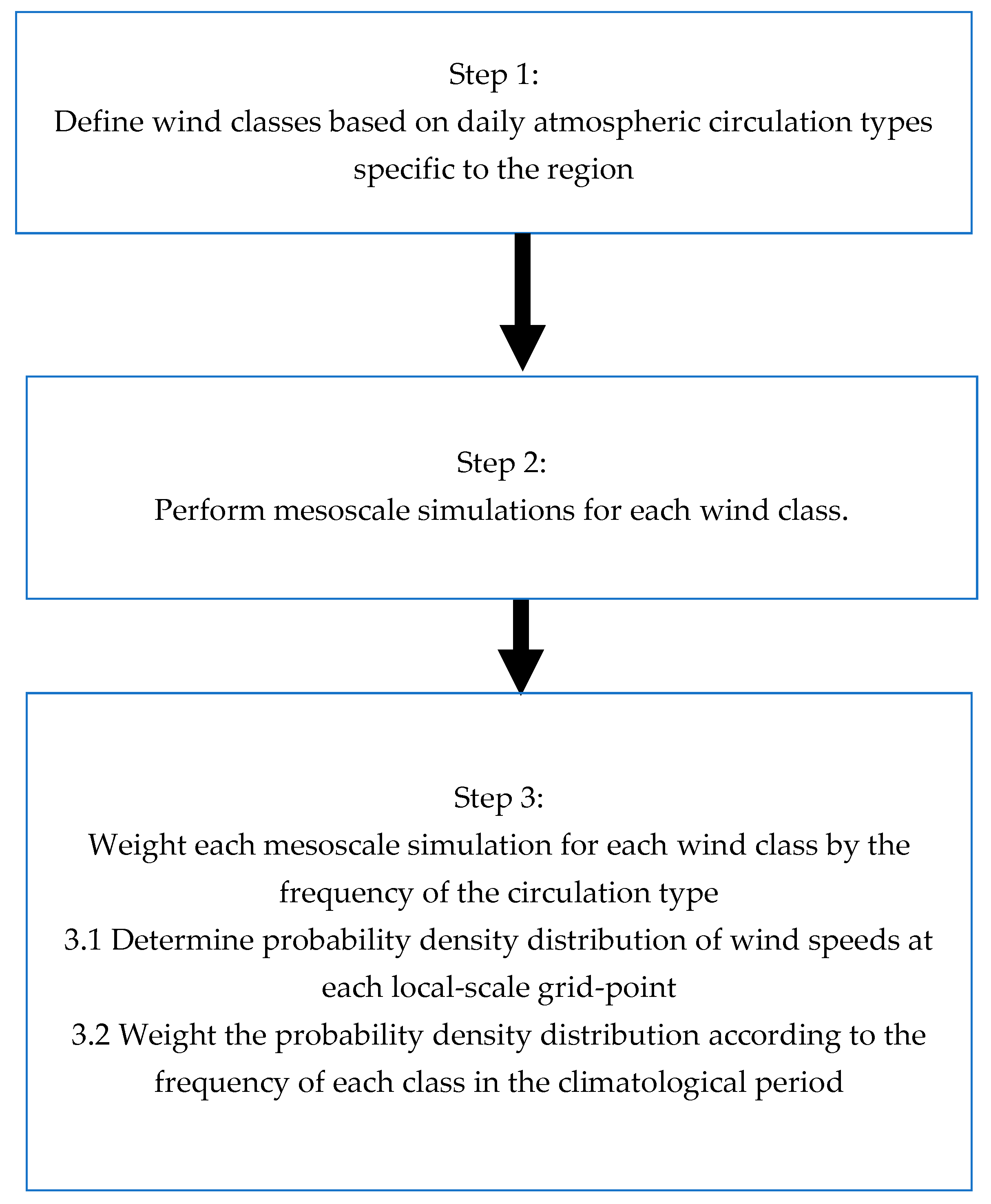
Figure 1. Overview of the proposed statistical–dynamical downscaling method for developing high-resolution wind maps.
Wind 05 00007 g001
Figure 2. Maps of (a) Caribbean small island states and (b) the case study area, Trinidad and Tobago. In (a), Trinidad and Tobago is denoted by a transparent red box in the lower right segment of the map.
Wind 05 00007 g002
Figure 3. Atmospheric circulation types (CTs) in the Caribbean (indicated by wind-field arrows), and the corresponding mean wind speeds (as colored contours) [29].
Wind 05 00007 g003
Figure 4. Representative monthly atmospheric circulation patterns (green arrows) (and wind classes) for CT 1 over a smaller region of the Caribbean. The legend’s vector length corresponds to 2.5 m s−1.
Wind 05 00007 g004
Figure 5. Range of correlations between each monthly pattern of each circulation type and its corresponding centroid.
Wind 05 00007 g005
Figure 6. Error vectors (in red) equal to the (a) difference between the derived long-term 10 m wind field created with seven wind classes (LT7) and the actual long-term mean (LT), and the (b) difference between the derived long-term field created with eighty-two wind classes (LT82) and the actual long-term mean (LT). The legend’s vector length corresponds to 0.25 m s−1.
Wind 05 00007 g006
Figure 7. The domain under consideration. The outermost boundaries denote the parent grid; d02 and d03 are the nested domains.
Wind 05 00007 g007
Figure 8. Wind speed map at 10 m AGL in and around Trinidad and Tobago.
Wind 05 00007 g008
Figure 9. Wind power density map at 10 m AGL in and around Trinidad and Tobago.
Wind 05 00007 g009
Figure 10. Histograms of 10 m level simulated wind speeds at the grid points closest to (A) Crown Point and (B) Piarco. The simulated pdf is represented by the black line, and the observed pdf is represented by the bar plots in each figure. The frequencies are represented as fractions.
Wind 05 00007 g010
Figure 11. Interannual variability in annual 10 m level mean wind speeds. Simulated wind speeds are in red and in situ data are in blue lines. Simulated wind speeds were taken from the grid points closest to (A) Crown Point and (B) Piarco. The horizontal dotted lines indicate the corresponding long-term means.
Wind 05 00007 g011
Figure 12. Wind speed map at 50 m AGL in and around Trinidad and Tobago.
Wind 05 00007 g012
Figure 13. Wind speed map at 80 m AGL in and around Trinidad and Tobago.
Wind 05 00007 g013
Figure 14. Simulated average vertical profiles of wind speeds at Crown Point and Piarco.
Wind 05 00007 g014
Table 1. Physical parameterizations used to configure WRF.
Physical ParameterizationName of the Parameterization Scheme
Planetary boundary layerYonsei University PBL scheme with topographic drag enabled
Surface layerMonin–Obukhov
Longwave radiationRRTM
Shortwave radiationDudhia
Land surface modelThermal diffusion
MicrophysicsWSM 3
CumulusBetts–Miller–Janjic (on d01 only; cloud formation is explicitly resolved on nests d02 and d03 (5 km and 1 km resolutions, respectively.)
Table 2. Climatological station information.
Station Name LocationElevationClosest Grid Point
Piarco, Trinidad 10.617 °   N ,   61.350 °   W 15 m 10.6182 °   N ,   61.3479 °   W
Crown Point, Tobago 11.150 °   N ,   60.833 °   W 12 m 11.1486 °   N ,   60.8286 °   W
Table 3. Comparison of the influences of the interannual variability on modeled wind data and measured data.
LocationInterannual Variability In
Wind SpeedWind Power Density (WPD)
Simulated (%)Measured (%)Simulated (%)Measured (%)
Crown Point(−11.6,13.6)(−19.3, 25.9)(−23.9, 40.3)(−47.7, 63.5)
Piarco(−10.7,18.9)(−16.3, 14.8)(−18.8, 44.3)(−27.4, 22.3)
Table 4. Wind speed shears between 50 m and 10 m, 100 m and 10 m, and 100 m and 50 m.
z 2   m   v s .   z 1   m Wind Speed Shear Exponents
Crown PointPiarco
50 m vs. 10 m0.2770.293
100 m vs. 10 m0.2660.299
100 m vs. 50 m0.2390.310
Disclaimer/Publisher’s Note: The statements, opinions and data contained in all publications are solely those of the individual author(s) and contributor(s) and not of MDPI and/or the editor(s). MDPI and/or the editor(s) disclaim responsibility for any injury to people or property resulting from any ideas, methods, instructions or products referred to in the content.