Abstract
This study examines output energy and efficiency of a torsional flutter harvester in gusty winds. The proposed apparatus exploits the torsional flutter of a rigid flapping foil, able to rotate about a pivot axis located in the proximity of the windward side. The apparatus operates at the “meso-scale”; i.e., the apparatus’ projected area is equal to a few square meters. It has unique properties in comparison with most harvesting devices and small wind turbines. The reference geometric chord length of the flapping foil is about one meter. Energy conversion is achieved by an adaptable linkage connected to a permanent magnet that produces eddy currents in a multi-loop winding coil. Operational conditions and the post-critical flutter regime are investigated by numerical simulations. Several configurations are examined to determine the output power and to study the effects of stationary turbulent flows on the energy-conversion efficiency. This paper is a continuation of recent studies. The goal is to examine the operational conditions of the apparatus for a potentially wide range of applications and moderate mean wind speeds.
1. Introduction
1.1. Literature Review and Motivation
Wind-based harvesting technologies are usually designed to supply energy to miniature sensors and small devices [1,2]. These applications are unsuitable to wind energy extraction at other scales.
The proposed apparatus is conceived for an application in the range designated as “meso-scale” wind energy. It concerns an apparatus with projected area equal to few square meters, which is typical of small vertical axis wind turbines such Savonius, Darreius and Gorlov [3]. This definition is based on the differentiation between the micro-scales of the small sensors, and the macro-scale of the horizontal axis wind turbines with swept areas of hundreds of square meters. The proposed apparatus is devoted to the needs of a single housing unit (few kW) or, similarly, the lighting of common spaces, footbridges, etc. The common task is scavenging energy at low flow speeds. Some examples are provided below to justify the motivation for this study.
Although some studies have examined the technical feasibility of installing meso-scale wind turbine devices in South Korea [4,5,6,7,8], this line of research mainly focuses on more traditional turbine types (e.g., Darreius). An attempt to improve this technology is provided by a device installed on a highway bridge that exploits both galloping vibrations at low wind speeds and deck vibrations, induced by traffic, to recover energy [9,10].
Meso-scale harvesters based on the principle of vortex-induced vibrations of multi-unit circular cylinders in water flows [11] have been considered. Harvesting devices, triggered by water axial flow instabilities [12], or by vortex-induced vibration of cylinders inside ventilation ducts [13,14], have been studied. Magnetic levitation has also been explored as a potential mechanism for energy conversion [15].
Moreover, exploitation of meso-scale “flutter mills”, using coupled bending-torsion flutter in wind flows (e.g., [16,17,18]), has been investigated. More specifically, a recent parametric study proposed the use of a pitching–heaving “foil turbine” at high Reynolds numbers [19]. Although the efficiency is estimated at about , this result is based on numerical computational fluid dynamics solvers that do not explicitly address the compliance of aeroelastic loads with the unsteady flutter formulation at moderate pitching amplitudes (e.g., [20]). Furthermore, this type of device requires a more complex design to accommodate for the coupled bending-torsion vibration. Supplementary study of the literature (e.g., [1,2,17]) also suggests that successful design of harvesters, exploiting aeroelastic flutter, are usually utilized to power miniature sensors (e.g., [21]).
Despite all these advancements, meso-scale applications and alternative solutions are still unexplored. Hence, there is still an opportunity for advancing basic research and developing a new technology, i.e., the apparatus discussed herein. The operating principle is inspired by pioneering work, examining the torsional flutter of a bluff body with “H-shaped” cross section [22,23]. Although the proposed apparatus performs worse compared to previous examples (e.g., [19]), it is a simpler device that is worthy of investigation.
1.2. Brief Description of the Apparatus
The harvesting device is presented in Figure 1.
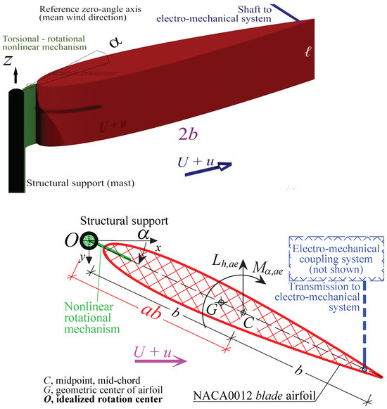
Figure 1.
Torsional flutter harvester: 3D schematics (top), 2D view on XY plane (bottom). The schematics of the electro-mechanical output power system may be found in Caracoglia [24].
It is composed of a rigid, symmetric and streamlined blade-airfoil of aspect ratio , with ℓ span-wise length and b half-chord length. The blade can rotate on a horizontal plane about a pivot axis “O” (angle in Figure 1). For flutter to occur [24], the position of the flapping pivot axis must vary between the windward edge, i.e., relative distance measured from the mid-chord point C towards the front of the airfoil (dimensionless distance ) and a point close to the aerodynamic center [25] of the blade-airfoil (). It is noted that in Figure 1 coincides with the pivot position at the mid-chord point C, while pivot positions with are situated towards the tail of the airfoil.
The torsional flutter harvester becomes active beyond a critical flutter speed threshold, usually above 10 m/s.
The kinetic energy associated with the flapping vibration is converted to electric energy by a mechanical transmission system connected to a permanent magnet that slides inside a multi-loop coil; this design is inspired by similar harvesting devices [9,15]. The shaft of the mechanical transmission system is visible in Figure 1; it is located at , on the tail side measured from the mid-chord point C. The eddy currents that are produced in the coil system by variations of flapping angular motion are stored in a battery for future re-use. An in-depth description and detailed schematics are not reported herein but may be found in Figure 1b and Section 3.3 of a previous paper [24].
1.3. Overview of Previous Studies
For the sake of completeness, the results from previous investigations are briefly described. Caracoglia [24] preliminarily evaluated the onset of torsional flutter in smooth wind flows, i.e., the critical flutter speed beyond which sustained vibration occurs. Caracoglia [24] solved a system of two nonlinear algebraic equations in dimensionless form; he shows that the reduced critical flutter velocity depends on a nonlinear inertia parameter. Interestingly, a very similar result may be found in a study on the flutter of pitching airfoils by Smilg [25]. Caracoglia [24] also concludes that, although the efficiency may be low, the design of the apparatus is very simple and advantageous. Furthermore, the same study examines the output power of the combined electro-mechanical system, coupling the flapping airfoil mechanism with an eddy current apparatus. In the post-critical stages, the nonlinear effects, necessary to maintain limit-cycle angular vibrations, are enforced by a torsional mechanism, combining a linear and a cubic restoring torque mechanism, i.e., a Duffing-type spring model. The same operating principle as the “nonlinear energy sink” [26] is utilized to achieve the nonlinear restoring torque effect.
In a subsequent study [27], the numerical model was expanded to evaluate the post-critical stability of the harvester as well as the output power, produced via flutter angular vibrations. The simulations account for stationary turbulence and load perturbations. Caracoglia [28] studied the performance of the harvester in a non-stationary wind flow, with intermittent “mean” wind speed slow fluctuations accompanied by fast turbulence perturbations. This flow condition is possible in urban environments that are influenced by the presence of buildings, obstacles, etc.; this study concludes that flutter and post-critical vibrations may still be triggered although the critical wind speed, beyond which the apparatus becomes operational, may double.
In an attempt to improve the performance of the harvester in non-stationary wind flows, Caracoglia [29] studied the design of a possibly more comprehensive “nonlinear rotational mechanism” (Figure 1), simulated by a hybrid Duffing–van der Pol restoring torque model with negative nonlinear damping effect. The study concludes that the van der Pol effect is beneficial in non-stationary flows, although it does not sensibly improve the performance.
Finally, Qin and Caracoglia [30] recently expanded the results in Ref. [24] to derive a closed-form formula that estimates the minimum operational conditions of the apparatus at flutter onset in the presence of stationary turbulent winds.
1.4. Study Objectives
Numerical investigations are carried out to study various configurations and to examine the feasibility of an “optimal” solution that could be used for future experimental validation and prototype design, currently in the planning stage. This study also serves as verification of the dynamic model, coupled with an energy-conversion model, by numerical analysis. Specifically, the following model parameters will be varied: (i) two structural parameters, the dimensionless cubic stiffness coefficient of the Duffing model and the nonlinear damping coefficient of the van der Pol model, (ii) the electro-motive coupling coefficient of the eddy current power circuit [9] and (iii) the generalized impedance of the power circuit.
2. Modeling Background
2.1. Dynamic Post-Critical Regime
A nomenclature table may be found at the end of this document, summarizing the symbols used in the following derivations.
The post-critical flutter behavior depends on torsional rotation and derivative with respect to dimensionless time with dimensional t time; is the angular frequency of the linear torsional flapping oscillator and is the total polar mass moment of inertia of the flapping foil about O. The dynamic equilibrium flapping equation is [28]:
Linear structural damping is simulated through damping ratio . Nonlinear restoring torque is simulated by the function with and [29]. Noting that the moment arm is from the pivot O to the leeward edge in Figure 1, the aeroelastic torque is about pivot O. Furthermore, the electro-motive torque is , in which is the dimensional output current of the power system, is the dimensionless output current, is the resistance of the power circuit and and is the dimensional electro-mechanical coupling coefficient (newton/ampère, N/A) [28].
The moving coil produces magnetic induction and interacts with a moving shaft, translating inside a coil (refer to Figure 1c and Section 3.3 in Ref. [24]). The dimensional moment arm of the eddy current, electro-magnetic torque is also about the pivot O, ; this arm becomes if the pivot axis coincides with the leeward edge and [].
In stationary turbulent flow, the instantaneous value of the wind speed becomes with being the along-wind turbulence component. The turbulence is fully correlated across the harvester since the reference planar or diagonal dimension is small compared to the atmospheric turbulence integral scales [28]. After normalization , the squared value of the wind speed, , can be adapted and inserted into torque to produce a multiplicative stochastic perturbation, e.g., similar to Pospíšil et al. [31].
From Equation (1), the dynamic equation of the flapping angle is consequently found for a pivot rotation axis at the windward edge () in Figure 1 [24,28]:
In Equation (2) ; , , and are four time-dependent aeroelastic states; is the inertia parameter [24] and is the air density. The parameter is derived from Ref. [32] and accounts for three-dimensional flow effects on the lift and the torque.
On the left-hand side of Equation (2), the nonlinear function is again used to differentiate between the Duffing model ( only) and the hybrid Duffing–van-der-Pol one (both and ). In Equation (2), the dimensionless coefficient controls the -dependent interaction between the flapping angle and the induced current ; the quantity is described in Equation (6).
2.2. Stochastic Differential Vector-Equation and Numerical Solution by Monte-Carlo Methods
Two types of perturbations are considered. First, along-wind turbulence is random. It is simulated in Equation (2) as a Wiener process [33] of independent Gaussian increments with standard deviation .
Second, load perturbations are also introduced, i.e., errors due to modeling simplifications since the aerodynamics of the NACA0012 cross-sectional profile is approximated by a flat plate airfoil. Specifically, the concept “torque load error” is employed; the perturbation is linked to the parameter of the unsteady torque (via Wagner function [34]). Consequently, is also random, with mean value and zero-mean, Gaussian variation of standard deviation .
The independence between the two perturbations is justified. Turbulence perturbation is related to the special operational conditions under atmospheric boundary layer winds. Aeroelastic load perturbations are related to load modeling simplifications, i.e., the use of the flat plate aerodynamic theory to describe the loads.
The dynamic equation (Equation (2)) is combined with additional equations representing the Faraday’s law of the power circuit and the temporal evolution of the aeroelastic states. It is subsequently transformed to an Itô-type [33] stochastic differential equation:
In Equation (3), is the state vector; includes both physical, aeroelastic states and dimensionless output current . In Equation (3), the scalar, Wiener noise separately addresses turbulence perturbation from the noise , used for aeroelastic torque perturbation. Quantity is a nonlinear vector function; is a nonlinear turbulence diffusion vector function. is a constant, diffusion matrix that controls the load perturbation and depends on the standard deviation of torque load error, .
The complete derivations of the stochastic differential equation in Equation (3) may be found in a previous study [27]; they are not repeated herein for the sake of conciseness. Specifically, the nonlinear drift vector , the matrix and the nonlinear diffusion vector are, respectively, described in Equations (11), (13) and (14) of paper [27].
Equation (3) is resolved in weak form by numerical integration [35], i.e., by collecting samples of the solutions over time . Appropriate initial conditions are imposed on the probability distribution of at . Monte-Carlo sampling is used to approximate the second Moment Lyapunov Exponent (2MLE) of the sub-vector of . After collecting the Monte-Carlo realizations, mean-square instability requires that the 2MLE of be strictly positive [36]:
In the above equation, is the expectation operator, applied to the Euclidean norm of the vector that is evaluated at time ; time is sufficiently large; i.e., Equation (4) approximates the limit as [36]. The 2MLE is commonly utilized to study asymptotic stability of nonlinear stochastic systems [36,37]. The largest Lyapunov exponent is a measure of dissipation, i.e., nonlinear damping effects. Specifically, as leads to an asymptotically stable system, in which any initial perturbation leads to vibrations that are fully dissipated. Equation (4) examines the variance of the stochastic vector ; this condition corresponds to the mean-square stability, i.e., the almost sure stability of a stochastic system [37,38]. This definition of stochastic stability is preferable since it usually leads to a more stringent stability criterion, compared to the analysis of the “drift”, i.e., .
Initial flapping conditions are necessary to examine the stability. They are imposed by considering an initial flapping angular motion at . This initial amplitude of is set to a random value with zero mean and standard deviation equal to , coincident with small, realistically plausible angular deviations from the static equilibrium of the blade-airfoil; this value is compatible with typical angle perturbation effects, associated with buffeting angular motion due to incoming flow turbulence.
In this study, 2MLE is employed to detect post-critical operational conditions. The numerical solution of Equation (3) is repeated 200 times by Monte-Carlo sampling and step-by-step integration to find the relevant statistical moments [35].
2.3. Output Power Estimation
Because of Equation (3), the post-critical output power is a random process. The output power expectation at sustained flapping is [28]:
where is the variance of , noting that . The “dimensionless electro-mechanical coupling coefficient” is
3. Description of the Apparatuses
Three harvester configurations are examined, with flapping pivot axis at the apex of the blade-airfoil () and ().
The three reference “Types” are selected from previous studies [24]. The main properties are described in Table 1. In this table, quantities such as angular frequency and damping ratio are the properties of the linearized dynamic equation of the harvester. The physical parameters of the three configurations in Table 1 are based on a series of preliminary studies described in Ref. [24].

Table 1.
Harvester and wind turbulence properties.
Furthermore, in Table 1 the nonlinear stiffness parameter of the Duffing model is set to a constant in (with ) and in the sixth column of Table 1. By contrast, in the case of or the hybrid Duffing–van-der-Pol model [29] a non-zero, nonlinear damping parameter (seventh column of Table 1) is used with in .
The wind flow is stationary and turbulent, with mean speed m/s and turbulence intensity between 2% (smooth flow) and 20% (high turbulence) (ninth column of Table 1).
Finally, aeroelastic load perturbation is considered in Table 1. It is simulated, independently of turbulence effects, as a Gaussian noise applied to the load parameter [24] of the unsteady Wagner indicial function [34], with mean value equal to [39] and standard deviation equal to . This standard deviation corresponds to a coefficient of variation equal to about 23%.
4. Discussion of the Results
The expected value of the output power (Equation (5)) is evaluated, accounting for mean speed U, stationary Gaussian inflow turbulence u (or ) as well as load modeling errors. The three representative devices are used (types 0, 1 and 2 in Table 1). Optimization is carried out by separately considering Duffing and hybrid Duffing–van der Pol restoring torque mechanisms, and by varying wind turbulence as well as the properties of the eddy current energy-conversion system.
4.1. Reference Output Power Configuration
In the “reference output power configuration”, the properties of the power circuit are set to in Equation (6) and ; is the generalized impedance of the power circuit ( resistance, inductance) [24].
4.1.1. Duffing Restoring Torque Mechanism
The first scenario analyzes a smooth flow field, typical of open terrain atmospheric conditions. This example represents the basic configuration. Since the Wiener model from Equation (3) is used, very low turbulence of intensity is introduced. Figure 2 presents the post-critical flutter analysis, evaluating both (a) 2MLE and (b) mean output power . The mean flow speed is set to m/s.

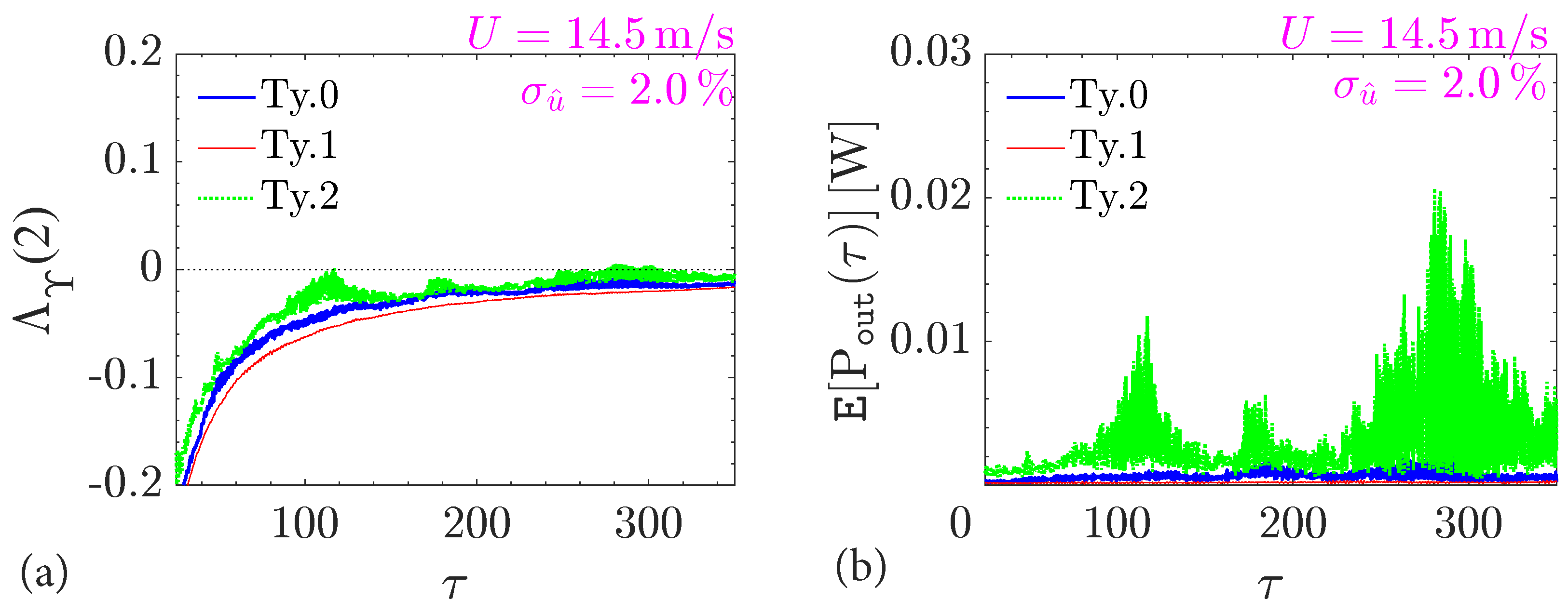
Figure 2.
Post-critical flutter analysis by (a) 2MLE and (b) mean output power —mean flow speed m/s, smooth flow (turbulence with ).
In the output power graphs of Figure 2b and subsequent figures (Figure 3 and Figure 4, etc.) the 2MLE and mean output power are only shown beyond , since must be large in Equation (4).
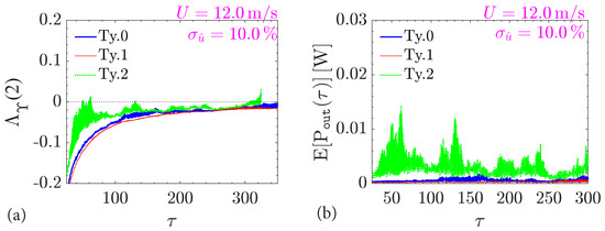
Figure 3.
Post-critical flutter analysis by (a) 2MLE and (b) mean output power —mean flow speed m/s, moderate turbulence with .
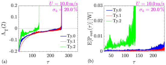
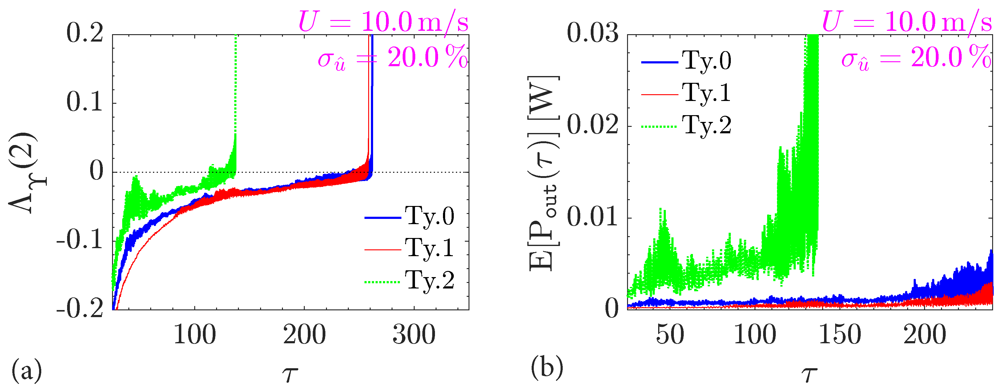
Figure 4.
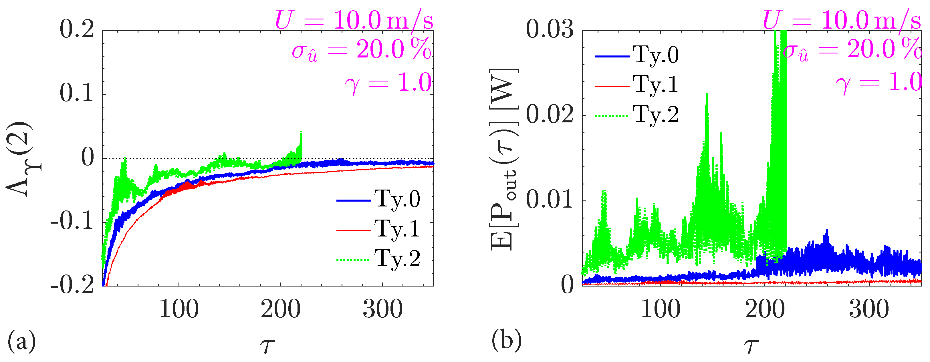
Post-critical flutter analysis by (a) 2MLE and (b) mean output power —mean flow speed m/s, high turbulence with .
In Figure 2a, types 0 and 1 are still stable and unable to produce energy in this velocity range, as indicated by the negative 2MLE with at , i.e., asymptotically. By contrast, the output current is not negligible in the case of the type-2 apparatus, with an overall fair efficiency and W (Figure 2b); the 2MLE is marginally positive in Figure 2a (dotted line).
At lower mean wind speeds U, flutter is not activated and no relevant output power is recorded. At higher U values, not shown in the figure panels, the behavior is similar to Figure 2 although the output power production is still very small. Since the apparatus is designed to be operational in the range of flow speeds below 15 m/s, they are less important and not documented in the following.
Figure 3 examines the moderately turbulent wind field conditions with turbulence intensity . Higher turbulence is conducive of more susceptibility to buffeting and torsional flutter, which is beneficial for energy conversion. Specifically, Figure 3a demonstrates that m/s can lead to instability for the type-2 apparatus, with after crossing the zero horizontal axis as ; also follows a divergent growth. The output power analysis is limited to the range of in Figure 3b, in which the type-2 system approaches the unstable flutter operational condition; the produced output power is very low, W (Figure 3b), although it is observed at a lower U compared to the smooth-flow case in Figure 2b. As before, both type-0 and type-1 apparatuses are not inadequate; i.e., the parameters in Table 1 are not suitable.
As flow turbulence is incremented (Figure 4), the ability to trigger torsional flutter appears enhanced and occurring at lower wind speeds. This trend is evident in Figure 4 which describes an urban exposure scenario with very large turbulence of intensity . Unstable behavior and post-critical flutter flapping are noted at mean flow speed m/s, triggering the energy-conversion mechanism. This effect produces, on average, W for the type-2 apparatus in Figure 4b; the plot of output power is interrupted at as numerical integration issues arise beyond this point. This “sudden overshoot” is noticeable for all the three types that exhibit a large, positive and divergent at different values. This issue is likely due to numerical integration accuracy [28], and it is noted in other cases (also refer to the discussion in Section 5.3).
The energy conversion in Figure 4b is three times larger in comparison with smooth-flow conditions, which was also observed at larger mean wind speeds with m/s. Furthermore, non-negligible conversion is noticeable for type-0 and type-1 apparatuses in Figure 4b, suggesting that turbulent flows are preferable. The overall efficiency is still low, with W for the Type-2 apparatus. This remark confirms the necessity for further investigation to find a better combination of structural and aerodynamic design parameters.
4.1.2. Hybrid Duffing–van der Pol Restoring Torque Mechanism
As in Section 4.1.1, various flow field scenarios are considered, from smooth flow to highly turbulent flow. In the case of the hybrid Duffing–van der Pol torque mechanism, it is necessary to specify the nonlinear damping coefficient in the function . A previous study [29] has explored some values of . Using the preliminary results, the range is further examined in this paper.
In the case of , the unstable post-critical regimes at various turbulence intensities are marginally affected by the introduction of nonlinear damping; the and are almost the same as the ones observed with the Duffing restoring torque mechanism in Section 4.1.1. Specifically, W is noted for the type-2 apparatus in smooth flow conditions at mean flow speed m/s (similarly to Figure 2), and W is noted for the type-2 apparatus in moderately turbulent flows at m/s (similarly to Figure 3). Therefore, a detailed graphical report on the examples with is omitted for the sake of brevity.
By contrast, some positive influence on the performance is observed in Figure 5, documenting the case with , m/s and high turbulence (). The mean output power of the type-2 apparatus is larger () than the power presented in the homologous figure without the van der Pol negative damping effect ( in Figure 4); the relative output power increment is . Furthermore, the type-0 apparatus exhibits a non-negligible output power value in Figure 5.
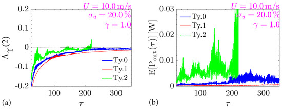
Figure 5.
Post-critical flutter analysis of a hybrid Duffing–van der Pol apparatus by (a) 2MLE and (b) mean output power —mean flow speed m/s, high turbulence with .
The reason for using a larger is dictated by the need for triggering the nonlinear damping term and for a better efficiency. Specifically, the damping term depends on the square value of the flapping amplitudes in the function .
Unfortunately, as suggested by previous research [29], a mechanism with a large may be impractical. A modification of the mechanism at the pivot rotation axis (Figure 1) might require a more complex design of the hybrid apparatus. Contrary to the Duffing model that can possibly be manufactured by adaptation of the “nonlinear energy sink” concept and hardware (refer to Section 2.6 in Vakakis et al. [26]), a nonlinear, negative damping effect is more difficult to reproduce. Furthermore, the negative sign in equation , used to characterize , implies that the kinetic energy may partly be lost or dissipated prior to its conversion to electric energy.
Consequently, the final investigation in Section 4.2 will exclusively examine the Duffing model and a modified configuration that enhances output power.
4.2. Modified Configuration to Enhance Output Power
The modified configuration examines the variation of the electric quantities, i.e., an increment of both and . A promising influence of these modifications was noted in a previous study [24]. Figure 6 first analyzes the exclusive increase of to under a smooth flow wind scenario, similar to Figure 2. On one side, the variation alone may lead to the potential increment of output power in Equation (5). However, a larger also introduces in Equation (1) a larger, negative electro-motive torque, opposing the growth of the aeroelastic flapping. Therefore, these two effects are contrasting and must be carefully balanced [24,28].
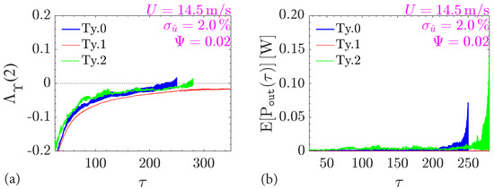
Figure 6.
Modified Duffing-type configuration with : (a) 2MLE and (b) mean output power —mean flow speed m/s, smooth flow (turbulence with ).
Figure 6b suggests that, at mean flow speed m/s, the performance worsens compared to Figure 2b because the mean output power is about W only. It also demonstrates that unstable flutter can possibly be extended to the type-0 apparatus, which is also suitably active other than the type-2 device in Figure 6b. Nevertheless, a balance between and is still not evident.
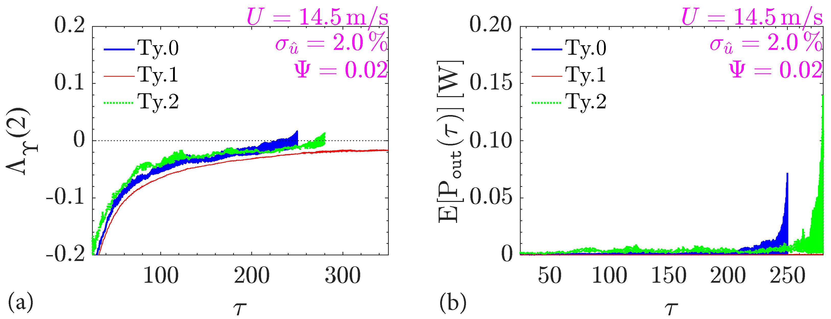
This balance is examined in Figure 7, in which both parameters are increased as and ; this figure evaluates the instability at mean speed m/s. Interestingly, the mean output power of the type-2 apparatus, the only apparatus that once again exhibits post-critical flapping in Figure 7a with , significantly increases in comparison with the reference configuration (Figure 2b). W quadruples the type-2 apparatus in Figure 7b. Unfortunately, type-0 and type-1 devices are still not efficient.
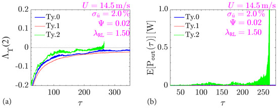
Figure 7.
Modified Duffing-type configuration with and : (a) 2MLE and (b) mean output power —mean flow speed m/s, smooth flow (with ).
5. Conclusions
5.1. Summary
This study continues the numerical investigations on the performance of a torsional flutter harvester, operating in stationary turbulent winds. The simulations suggest that highly turbulent winds are preferable. Furthermore, they provide evidence that the generalized impedance coefficient of the eddy current power circuit may have a relevant and positive influence on the efficiency of the apparatus, mainly type-2.
5.2. Main Findings
The main findings can be summarized as follows:
- The second configuration in Table 1, “Ty.2”, appears to be the most versatile and engaged by angular vibrations across all the various scenarios that have been examined. Output energy is often one order of magnitude larger than other configurations; for example, refer to Figure 2b versus Figure 4b. The “Ty.0” potentially becomes a viable alternative at high turbulence intensities and if and only if the hybrid Duffing–van der Pol mechanism is considered (e.g., Figure 5b).
- Flow turbulence tends to have a positive effect on the vibration onset by preceding the occurrence of angular motion, especially for “Ty.2” apparatus (Figure 2a versus Figure 4a). The operational range of the “Ty.2” harvester increases contingent on a reduction of mean wind speed by about . Nevertheless, the latter beneficial effect is observed at large turbulence intensities () that are possible in an urban wind exposure.
- For a hybrid Duffing–van der Pol torque mechanism, a nonlinear damping coefficient is recommended. Although moderate, post-critical flapping amplitudes (below ) are desirably enforced to avoid flow separation from the surface of the blade-airfoil, this range of amplitudes does not guarantee a notable effect on the performance.
- Larger values of in the hybrid Duffing–van der Pol torque mechanism are theoretically unrealistic [29] since they may be accompanied by larger angular flapping amplitudes that are more difficult to achieve; energy redistribution in the hybrid device reduces the energy transferred to the eddy current system, by dissipation term in the function . This loss is noticeable, for example, in Figure 5b, compared to Figure 4b where the apparatus is equipped with a cubic Duffing setup only. Design of a hybrid harvester is discouraged.
- The study investigated the influence of electro-mechanical coupling and generalized impedance () on the harvester’s output power across various configurations. Section 4.2 reveals the crucial role of the impedance on the electro-motive torque that couples with the aeroelastic torque in Equation (1). A noteworthy increment of output power is observed in Figure 7b, equal to about one Watt, which is a promising result.
5.3. Outlook
Future studies will continue the examination of generalized impedance for a more comprehensive optimization of the apparatus. The use of multi-layered (i.e., stacked) blade-airfoils may be considered to enhance the harvester’s output [40]. Investigations by wind tunnel experiments and computational fluid dynamics studies have also been planned; both studies are under way. Results will be reported in the near future.
Nonlinear aeroelastic load modeling [41] will also be considered to replicate post-critical angular vibration regimes at larger amplitudes, .
Numerical integration issues have been reported in Figure 4a. The overshoot behavior was described earlier. The numerical solver employed herein is the Euler–Maruyama method [35]. This method is the simplest scheme for solving differential equations. The Euler–Maruyama solution converges weakly with order one under relatively mild conditions [38]; it is frequently utilized to generate samples of the solution. In this specific application, i.e., in Equation (3), the time step was set to to balance the computing time without compromising accuracy. This issue cannot be alleviated by further reducing the time step. Since the physical problem under consideration deals with dynamic stability and Equation (3) is moderately nonlinear, there is an issue with algorithmic convergence. The problem is primarily linked to the standard deviation of the Wiener process increments , associated with turbulence perturbations. While the numerical solution is marginally impacted at low turbulence, the undesirable influence becomes evident at larger intensities (Figure 4a). Attenuating this issue is possible by resorting to other numerical methods with stronger convergence (e.g., Milstein method [38], Leimkuhler–Matthews method [42]) but also a more complex algorithmic implementation. Although implementation is advisable, it has not been pursued herein. The numerics are less important in the context of this study, aiming at the identification of performance regimes only. Future experimental testing will also serve for verification of the numerical methods.
Funding
This material is based in part upon work supported by the National Science Foundation (NSF) of the United States of America, Award CMMI-2020063. Any opinions, findings and conclusions or recommendations are those of the author and do not necessarily reflect the views of the NSF.
Institutional Review Board Statement
Not applicable.
Informed Consent Statement
Not applicable.
Data Availability Statement
The data that support the findings of this study are available from the corresponding author upon reasonable request.
Acknowledgments
L. Caracoglia gratefully acknowledges the support of the Universities of Trento, Perugia and the Polytechnic University of Bari (Italy) during his sabbatical leave in 2024. L. Caracoglia also gratefully acknowledges the organizers of the ERCOFTAC SIG41 2024 Symposium for the kind invitation.
Conflicts of Interest
The author declares no conflicts of interest.
Nomenclature
The following symbols are used in this manuscript:
| Roman Symbols | |
| Aspect ratio of the blade-airfoil | |
| a | Dimensionless position of the pivot “O” |
| Scalar Wiener noise for turbulence | |
| Scalar Wiener noise for load perturbation | |
| b | Half-chord width of the blade-airfoil |
| Mean value of random (exponent) parameter: | |
| I | Output current of the power system (A) |
| Polar mass moment of inertia of flapping foil about “O” (kg×m2 ) | |
| Reduced frequency, one-DOF flapping foil | |
| Impedance of output power circuit (Henries) | |
| ℓ | Span-wise length of the blade-airfoil |
| Aeroelastic torque (Nm) | |
| Electromotive torque (Nm) | |
| Diffusion matrix of load perturbation | |
| Nonlinear drift vector-function (drift) | |
| Resistance of output power circuit (Ohms) | |
| t | Time (s) |
| Nonlinear turbulence diffusion function | |
| U | Mean wind speed (m/s) |
| Along-wind stationary turbulence (m/s) | |
| Normalized along-wind stationary turbulence | |
| Random state vector | |
| z | Vertical axis coordinate |
| Greek Symbols | |
| Flapping angle of the blade-airfoil, about “O” | |
| Nonlinear dimensionless damping (van der Pol) | |
| Zero-mean Gaussian random perturbation about | |
| Normalized inertia parameter | |
| Structural damping ratio of the flapping foil | |
| Nonlinear restoring torque function | |
| Three-dimensional load & flow effect parameter | |
| Dimensionless induced current, power circuit | |
| Dimensionless cubic torsional stiffness (Duffing) | |
| Second moment Lyapunov exponent | |
| Generalized impedance of the power circuit | |
| Aeroelastic state () | |
| Aeroelastic state () | |
| Standard deviation of | |
| Standard deviation of | |
| Dimensionless time | |
| Discrete time instant used to find 2MLE | |
| Sub-vector of state vector | |
| Unsteady aeroelastic forcing function at | |
| Dimensional electro-mechanical coupling coeff. (N/A) | |
| Electro-mechanical coupling coefficient | |
| Angular vibration frequency (rad/s) | |
| Pulsation of the one-DOF flapping foil (rad/s) | |
| Abbreviations and Operators | |
| DOF | Degree of freedom |
| Expectation operator | |
| T | Transpose operator |
| 2MLE | Second-moment Lyapunov exponent |
References
- Priya, S.; Inman, D.J. Energy Harvesting Technologies; Springer Science: New York, NY, USA, 2009. [Google Scholar]
- Young, J.; Lai, J.C.S.; Platzer, M.F. A review of progress and challenges in flapping foil power generation. Prog. Aerosp. Sci. 2014, 67, 2–28. [Google Scholar] [CrossRef]
- Hau, E. Wind Turbines: Fundamentals, Technologies, Application, Economics, 3rd ed.; Springer: Berlin/Heidelberg, Germany, 2013. [Google Scholar]
- Ali, S.; Lee, S.M.; Jang, C.M. Techno-economic assessment of wind energy potential at three locations in South Korea using long-term measured wind data. Energies 2017, 10, 1442. [Google Scholar] [CrossRef]
- Ali, S.; Lee, S.M.; Jang, C.M. Forecasting the long-term wind data via Measure-Correlate-Predict (MCP) methods. Energies 2018, 11, 1541. [Google Scholar] [CrossRef]
- Ali, S.; Jang, C.M. Effects of tip speed ratios on the blade forces of a small H-Darrieus wind turbine. Energies 2021, 14, 4025. [Google Scholar] [CrossRef]
- Ali, S.; Park, H.; Noon, A.A.; Sharif, A.; Lee, D. Accuracy testing of different methods for estimating weibull parameters of wind energy at various heights above sea level. Energies 2024, 17, 2173. [Google Scholar] [CrossRef]
- Ali, S.; Park, H.; Lee, D. Structural optimization of Vertical Axis Wind Turbine (VAWT): A multi-variable study for enhanced deflection and fatigue performance. J. Mar. Sci. Eng. 2025, 13, 19. [Google Scholar] [CrossRef]
- Kwon, S.D.; Park, J.; Law, K. Electromagnetic energy harvester with repulsively stacked multilayer magnets for low frequency vibrations. Smart Mater. Struct. 2013, 22, 055007. [Google Scholar] [CrossRef]
- Le, H.D.; Kwon, S.D. An electromagnetic galloping energy harvester with double magnet design. Appl. Phys. Lett. 2019, 115, 133901. [Google Scholar] [CrossRef]
- Bernitsas, M.M.; Raghavan, K.; Ben-Simon, Y.; Garcia, E.M.H. VIVACE (Vortex Induced Vibration Aquatic Clean Energy): A new concept in generation of clean and renewable energy from fluid flow. J. Offshore Mech. Arct. Eng. 2008, 130, 041101. [Google Scholar] [CrossRef]
- Singh, K.; Michelin, S.; de Langre, E. Energy harvesting from axial fluid-elastic instabilities of a cylinder. J. Fluids Struct. 2012, 30, 159–172. [Google Scholar] [CrossRef]
- Gkoumas, K.; Petrini, F.; Bontempi, F. Piezoelectric vibration energy harvesting from airflow in HVAC (heating ventilation and air conditioning) systems. Procedia Eng. 2017, 199, 3444–3449. [Google Scholar] [CrossRef]
- Petrini, F.; Gkoumas, K. Piezoelectric energy harvesting from vortex shedding and galloping induced vibrations inside HVAC ducts. Energy Build. 2018, 158, 371–383. [Google Scholar] [CrossRef]
- Kecik, K.; Mitura, A.; Lenci, S.; Warminski, J. Energy harvesting from a magnetic levitation system. Int. J. Nonlinear Mech. 2017, 94, 200–206. [Google Scholar] [CrossRef]
- Matsumoto, M.; Mizuno, K.; Okubo, K.; Ito, Y. Fundamental Study on the Efficiency of Power Generation System by Use of the Flutter Instability. In Proceedings of the ASME 2006 Pressure Vessels and Piping/ICPVT-11 Conference, Vancouver, BC, Canada, 23–27 July 2006; Volume 9, pp. 277–286. [Google Scholar] [CrossRef]
- Shimizu, E.; Isogai, K.; Obayashi, S. Multiobjective design study of a flapping wind power generator. J. Fluids Eng. 2008, 130, 021104. [Google Scholar] [CrossRef]
- Pigolotti, L.; Mannini, C.; Bartoli, G.; Thiele, K. Critical and post-critical behaviour of two-degree-of-freedom flutter-based generators. J. Sound Vib. 2017, 404, 116–140. [Google Scholar] [CrossRef]
- Boudreau, M.; Picard-Deland, M.; Dumas, G. A parametric study and optimization of the fully-passive flapping-foil turbine at high Reynolds number. Renew. Energy 2020, 146, 1958–1975. [Google Scholar] [CrossRef]
- Theodorsen, T. General Theory of Aerodynamic Instability and the Mechanism of Flutter; Technical Report NACA-TR-496; National Advisory Committee for Aeronautics: Washington, DC, USA, 1934.
- Eugeni, M.; Elahi, H.; Fune, F.; Lampani, L.; Mastroddi, F.; Romano, G.P.; Gaudenzi, P. Numerical and experimental investigation of piezoelectric energy harvester based on flag-flutter. Aerosp. Sci. Technol. 2020, 97, 105634. [Google Scholar] [CrossRef]
- Ahmadi, G. An oscillatory wind energy converter. Wind Eng. 1979, 3, 207–215. [Google Scholar]
- Roohi, R.; Hosseini, R.; Ahmadi, G. Parametric study of an H-section oscillatory wind energy converter. J. Ocean Eng. 2023, 270, 113652. [Google Scholar] [CrossRef]
- Caracoglia, L. Modeling the coupled electro-mechanical response of a torsional-flutter-based wind harvester with a focus on energy efficiency examination. J. Wind Eng. Ind. Aerodyn. 2018, 174, 437–450. [Google Scholar] [CrossRef]
- Smilg, B. The instability of pitching oscillations of airfoils in subsonic incompressible potential flow. J. Aeronaut. Sci. 1949, 16, 691–696. [Google Scholar] [CrossRef]
- Vakakis, A.F.; Gendelman, O.V.; Bergman, L.A.; McFarland, D.M.; Kerschen, G.; Lee, Y.S. Nonlinear Targeted Energy Transfer in Mechanical and Structural Systems (Part I); Springer: Dordrecht, The Netherlands, 2008; ISBN 978-1-4020-9130-8. [Google Scholar]
- Caracoglia, L. Stochastic stability of an aeroelastic harvester contaminated by wind turbulence and uncertain aeroelastic loads. J. Wind Eng. Ind. Aerodyn. 2023, 240, 105490. [Google Scholar] [CrossRef]
- Caracoglia, L. Stochastic performance of a torsional-flutter harvester in non-stationary, turbulent thunderstorm outflows. J. Fluids Struct. 2024, 124, 104050. [Google Scholar] [CrossRef]
- Caracoglia, L. Improving output power of a torsional-flutter harvester in stochastic thunderstorms by Duffing–van der Pol restoring torque. ASME J. Risk Uncertain. Part B 2024, 10, 041204. [Google Scholar] [CrossRef]
- Qin, Y.; Caracoglia, L. Turbulence and flapping pivot axis effects on torsional flutter harvester efficiency by closed-form formula. J. Wind Eng. Ind. Aerodyn. 2025, 256, 105938. [Google Scholar] [CrossRef]
- Pospíšil, S.; Náprstek, J.; Hračov, S. Stability domains in flow-structure interaction and influence of random noises. J. Wind Eng. Ind. Aerodyn. 2006, 94, 883–893. [Google Scholar] [CrossRef]
- Argentina, M.; Mahadevan, L. Fluid-flow-induced flutter of a flag. Proc. Natl. Acad. Sci. USA 2005, 102, 1829–1834. [Google Scholar] [CrossRef] [PubMed]
- Itô, K. On Stochastic Differential Equations. In Memoirs of the American Mathematical Society; American Mathematical Society: Providence, RI, USA, 1951; Volume 4, ISBN 978-0-8218-1204-4. [Google Scholar] [CrossRef]
- Wagner, H. Über die entstehung des dynamischen auftriebes von tragflügeln (in German). Z. Angew. Math. Mech. 1925, 5, 17–35. [Google Scholar] [CrossRef]
- Kloeden, P.E.; Platen, E.; Schurz, H. Numerical Solution of Stochastic Differential Equations Through Computer Experiments; Springer: Berlin/Heidelberg, Germany, 1994; ISBN 978-3-540-57074-5. [Google Scholar]
- Xie, W.C. Monte Carlo simulation of moment Lyapunov exponents. J. Appl. Mech. 2005, 72, 269–275. [Google Scholar] [CrossRef]
- Xie, W.C. Dynamic Stability of Structures; Cambridge University Press: New York, NY, USA, 2006. [Google Scholar]
- Grigoriu, M.D. Stochastic Calculus: Applications in Science and Engineering; Birkhäuser: Boston, MA, USA, 2002; ISBN 978-0-8176-4242-6. [Google Scholar]
- Jones, R.T. The Unsteady Lift of a Finite Wing; Technical Note NACA-TN-682; National Advisory Committee for Aeronautics: Washington, DC, USA, 1939.
- Roccia, B.A.; Verstraete, M.L.; Ceballos, L.R.; Balachandran, B.; Preidikman, S. Computational study on aerodynamically coupled piezoelectric harvesters. J. Intell. Mater. Syst. Struct. 2020, 31, 1578–1593. [Google Scholar] [CrossRef]
- Dunn, P.; Dugundji, J. Nonlinear stall flutter and divergence analysis of cantilevered graphite/epoxy wings. AIAA J. 1992, 30, 153–162. [Google Scholar] [CrossRef]
- Leimkuhler, B.; Matthews, C. Rational construction of stochastic numerical methods for molecular sampling. Appl. Math. Res. eXpress 2012, 2013, 34–56. [Google Scholar] [CrossRef]


Disclaimer/Publisher’s Note: The statements, opinions and data contained in all publications are solely those of the individual author(s) and contributor(s) and not of MDPI and/or the editor(s). MDPI and/or the editor(s) disclaim responsibility for any injury to people or property resulting from any ideas, methods, instructions or products referred to in the content. |
© 2025 by the author. Licensee MDPI, Basel, Switzerland. This article is an open access article distributed under the terms and conditions of the Creative Commons Attribution (CC BY) license (https://creativecommons.org/licenses/by/4.0/).