Trends and Interdependence of Solar Radiation and Air Temperature—A Case Study from Germany

Abstract

This study characterizes the spatiotemporal solar radiation and air temperature patterns and their dependence on the general atmospheric circulation characterized by the North Atlantic Oscillation (NAO) Index in Germany from 1991 to 2015. Germany was selected as the study area because it can be subdivided into three climatologically different regions: the North German lowlands are under the maritime influence of the North and Baltic Seas. Several low mountain ranges dominate Germany’s center. In the south, the highest low mountain ranges and the Alps govern solar radiation and air temperature differently. Solar radiation and air temperature patterns were studied in the context of the NAO index using daily values from satellite and ground measurements. The most significant long-term solar radiation increase was observed in spring, mainly due to seasonal changes in cloud cover. Air temperature shows a noticeable increase in spring and autumn. Solar radiation and air temperature were significantly correlated in spring and autumn, with correlation coefficient values up to 0.93. In addition, a significant dependence of solar radiation and air temperature on the NAO index was revealed, with correlation coefficient values greater than 0.66. The results obtained are important not only for studies on the climate of the study area but also for photovoltaic system operators to design their systems. They need to be massively expanded to support Germany’s climate neutrality ambitions until 2045.

1. Introduction

Changes in atmospheric transmission due to variations in cloudiness and aerosol concentration are the main factors causing trends in incoming solar radiation on a horizontal surface (SIS) penetrating the atmosphere and finally being available at the Earth’s surface for the generation of solar energy.

Due to aerosol–cloud interactions and aerosol and water vapor’s indirect effects on SIS, these factors are not mutually exclusive in explaining SIS changes. In order to investigate their influence, a study was carried out on the Mediterranean area as this region is one of the maritime areas with very high relative humidity and the largest aerosol loads in the world [1]. The authors used satellite data, specifically CERES (Clouds and the Earth’s Radiant Energy System) SYN1deg products. Their results show that the spatial distribution of aerosol and water vapor are closely linked to the spatial distributions of its effects on solar radiation. The air constituents cause a SIS reduction between 2.0–8.0% due to aerosol and 11.5–15.0% due to water vapor effects. The authors found the greatest effects of aerosol and water vapor on SIS in the period from July to September.

Variations in SIS also cause variations in surface air temperature (TAS). Although SIS warms the air only during the day, its variability is related to the variability of daily TAS amplitude on monthly and decadal time scales [2].

Since data records are available up to 1970, a decrease in TAS due to the reduced input of SIS was detected [3]. The authors combined the temperature data with radiation data and additional components of the hemispheric energy budget. The relationship between the change in SIS and the change in TAS was applied to the reported trends in direct solar radiation, revealing a probable cause–effect relationship. Long time series of temperature have already been tested several times. For Europe, the annual frequency of cold extremes has decreased since 1961 by about 7%/100 yr, with heat extremes increasing by more than 10%/100 yr [4]. Compared to mean annual warming of about 2–3 K/100 yr, the coldest winter temperatures have increased three times as fast, resulting in a smaller seasonal range and fewer variable winters. Changes in the warmest summer temperatures since 1961 show large spatial variations, with rates of change ranging from slightly negative to 6 K/100 yr. The spatiotemporal TAS change in Germany from 1951–2015, especially in spring, shows an increase in TAS of 1.6 K [5].

An earlier study carried out at the Baseline Surface Radiation Network (BSRN) station Tartu–Tõravere (58°16′ N, 26°28′ E) in Estonia found a good correlation between SIS and TAS [6]. The study also revealed the influence of the NAO index (NI) on European weather patterns and the TAS and SIS variability. The results of this work are discussed again later.

Since weather and associated TAS have an impact on the performance and electrical efficiency of photovoltaic (PV) systems, there is an interest in analyzing TAS-induced changes in PV system performance [7,8]. The PV system efficiency decreases with lower latitudes due to higher TAS. A study conducted in West Africa found that a TAS increase of 1.5 to 3.0 K decreases PV power generation by nearly 3.8% [9]. In mountainous regions, the performance of PV systems increases with decreasing TAS at higher elevations [10]. It was recommended to monitor TAS during PV system operation and to compensate for TAS increases accordingly to stabilize system performance and increase electrical efficiency [11].

Since 2000, the annual electricity generation from solar energy in Germany has increased from about 1% to more than 9% [12]. The aim of PV system operators is the increasing use of solar energy to mitigate anthropogenic climate change. During the transformation of the energy sector from conventional to renewable energies, it is imperative to maintain the balance between the variable energy supplies from solar and wind and the energy demand. The weather-related impacts of increasing penetration of the energy mix with solar and wind were exemplified in a previous study [13]. However, an increasing share of solar and wind energy in the future energy mix increases the likelihood of times when variable renewables are scarce. The greatest probability of occurrence of these periods, which in Europe are called “Dunkelflaute events”, is winter [14]. This requires systems ensuring the base load of the energy supply.

Previous results [15] and newly available data stimulated the investigations reported in this paper. For the territory of Germany, we examined how variations in atmospheric circulation, expressed by the NAO index [16] and SIS, influence decadal TAS variability.

The abbreviations used in this manuscript are explained in Appendix A.

2. Materials and Methods

The analysis of the spatiotemporal SIS and TAS variability comprises the following steps: (1) Obtaining daily mean values of SIS and TAS with a horizontal resolution of 0.05° × 0.05° for the 25-year period 1991–2015, (2) investigating the spatiotemporal variability of both variables by means of trend analysis and analysis of their inter- and intra-annual variability, (3) correlating SIS and TAS, and (4) correlating SIS and TAS with NI. The results were converted to a 10-year period (decade) to make them comparable with results from other studies.

All steps of data preparation and analysis were performed with the Satellite Application Facility on Climate Monitoring (CM SAF) R Toolbox software [17] and the Mathworks (Natick, MA, USA) Matlab software, version 2021b.

All figures showing the results for the study area are oriented north-south and have a scale of 1 cm equals 165 km.

2.1. Data

Daily mean values from the Surface Solar Radiation Data Set–Heliosat (SARAH)–Edition 2.1 were used for SIS analysis [18]. They are available on a regular grid. The SIS data records are based on observations of the MVIRI and SEVIRI instruments on board of the first and second generations of METEOSAT satellites. Preparation and provision of SIS data were carried out by CM SAF [19]. Further details on the uncertainty of SIS are given in [20].

The daily mean TAS data records for the same period were taken from the HYRAS dataset [21], interpolated on the same grid as for SIS, and finally merged into one file containing all 25-year data records. This study [21] provides information on HYRAS data quality. Monthly NI means are available on the US National Weather Service’s Climate Prediction Center website [16].

2.2. Assessment of Spatiotemporal Variability

The spatiotemporal variability and the long-term development of SIS and TAS were estimated by calculating mean values over the study period (SIS_P, TAS_P) at the grid cells and the study area. Monthly averages identified the SIS (SIS_M) and TAS (TAS_M) changes over the year. The long-term change (trend) in SIS (SIS_T) and TAS (TAS_T) is quantified by multiplying the slope of the trend lines by the respective interval length. The significance of SIS_T and TAS_T was determined by applying the Mann–Kendall test at a confidence level of α = 0.05 [22].

In contrast to a previous study [23], the inter-annual variability (IAV) was not expressed in relative terms. To obtain absolute values that more clearly highlight the differences in magnitude between individual months and years, monthly and annual SIS_IAV and TAS_IAV values were calculated as the range (maximum minus minimum values) of differences in mean values.

2.3. Assessment of the Correlation between SIS and TAS

An immediate reaction of TAS to a change in SIS cannot be expected, as both natural and anthropogenic air pollution within the atmosphere lead initially to the absorption and scattering of SIS. A further reduction in SIS occurs due to the varying degree of coverage. [24]. Finally, TAS reacts to these influences. A study of the correlation between SIS and TAS can therefore only provide reasonable results for the four seasons. In addition, it should be considered that SIS values are available only for daylight hours, while TAS describes the course of air temperature over the whole day.

To find possible reasons for the relationship between SIS and TAS, data from NI were included in the correlation analysis. NI characterizes the atmospheric circulation between North America and Europe transporting air masses of different temperatures into the study area. NI is defined as the difference between the normalized winter air pressures at sea level in Lisbon and Stykkisholmur (Iceland) [25]. A positive NI is found if its contrast is higher than average due to a very low pressure over Iceland and a very high pressure over the Azores with strong westerly winds over the North Atlantic between 40° and 60° N. The corresponding circulation leads to mild winters and abundant rainfall over Europe to Siberia and the American East Coast, while over the Mediterranean to the Near East there is drought and relatively cold winters. With a negative NI, the pressure contrast between the Icelandic low and the Azores high is significantly reduced. This stands for weaker westerly winds and an occurrence of relatively mild and humid winters in the Mediterranean and cold and dry periods in Europe and on the American East Coast.

3. Results and Discussion

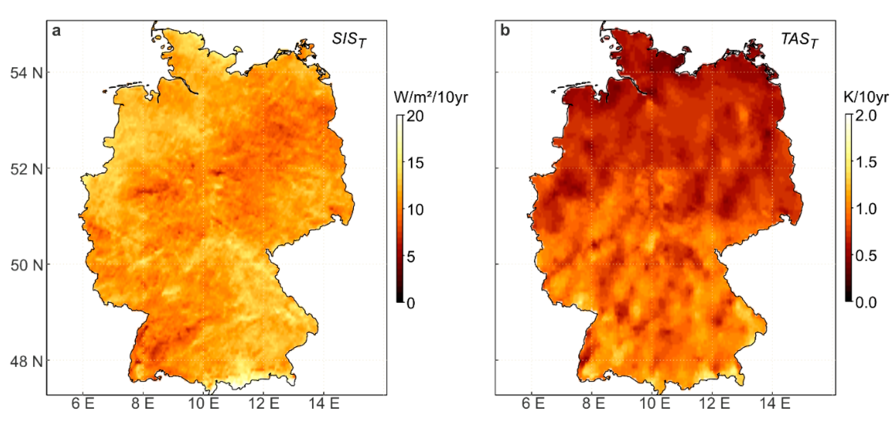
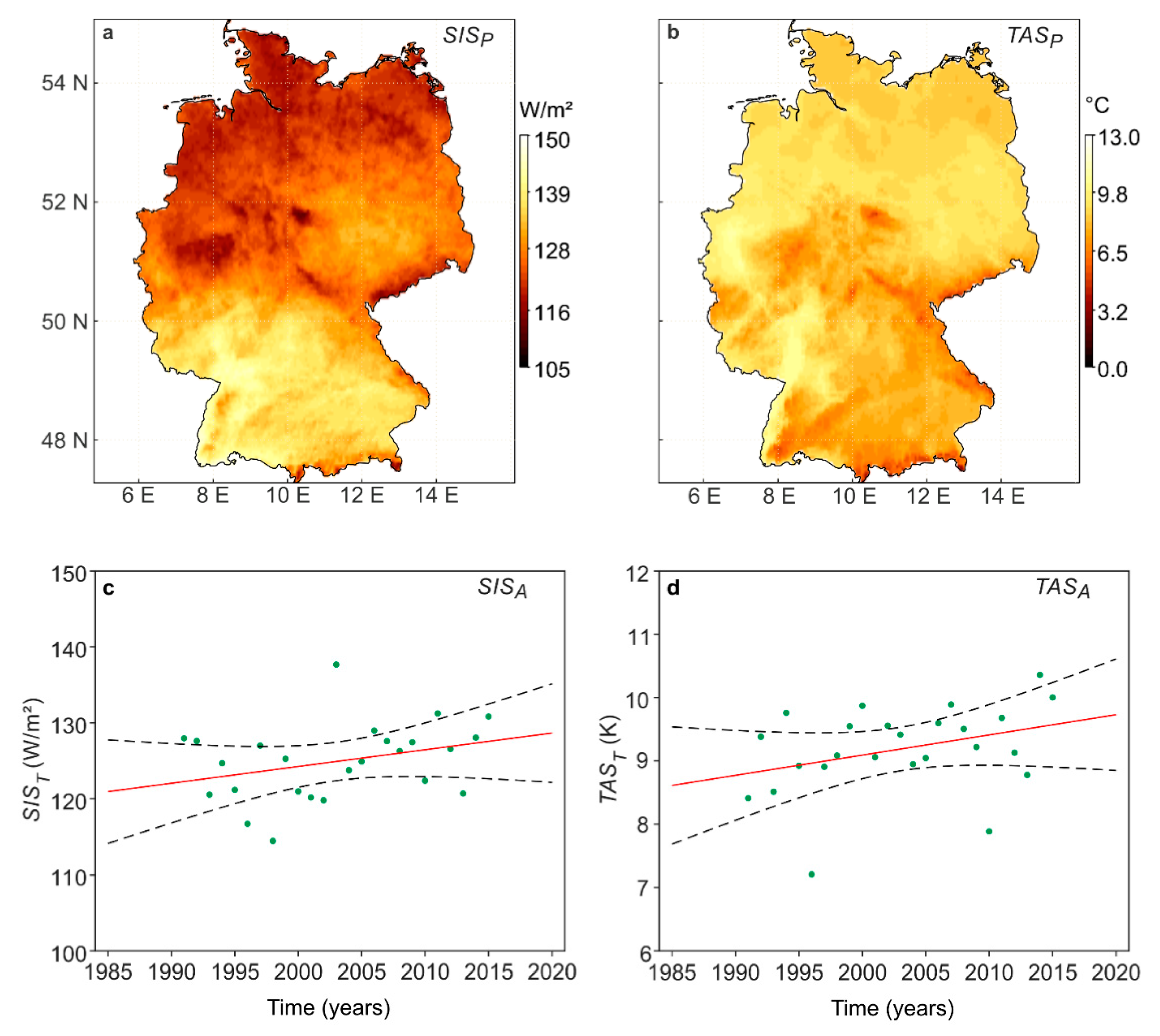
3.1. Annual Mean Pattern and Trends

Figure 1a shows the large-scale distribution of SIS_P with decreasing values from south to north. The large-scale pattern is superimposed by regional and local patterns, which are mainly influenced by orography [20].

Figure 1b shows the TAS_P pattern in the study area. Remarkably high values occur in the Upper and Lower Rhine Area at more than 12 °C. These areas are particularly favored in summer by the inflow of warmer air masses from the southwest. Due to the more continental influence with low cloud cover especially in summer, the area of Eastern Germany shows slightly increased values of just about 10 °C. The urban heat islands of Hamburg, Berlin, Halle/Leipzig, and Munich are obvious. Furthermore, the elevations of the low mountains in Central and Southern Germany (Harz, Thuringian, and Bavarian Forest, as well as the Swabian Alb) are recognizable by low annual average values of about 4 °C. The long-term change in annual mean values of SIS (SIS_A) in Germany is positive but non-significant (Figure 1c). Their total change SIS_T is 2.4 W/m²/10 yr. This result fits well with trends based on surface measurements in Central Europe reported in another study [26]. The relative standard deviation of SIS_A equals 3.9%, corresponding to an absolute value of 4.9 W/m². This matches with the findings of [27] who found a SIS_A variation with a relative standard deviation of 4–6% in most parts of Central Europe. A study of the spatiotemporal SIS variability over the Eastern Mediterranean in 1983–2013, using data records of SIS from the same source as used in this study, found a positive (brightening) and statistically significant SIS_T at the confidence level α = 95% with 2 ± 0.05 W/m²/10 yr, with on- and offshore being almost equal [28].

The long-term change in TAS annual mean values (TAS_A) is significantly positive (Figure 1d) with a total change in TAS_T of 0.32 K/10 yr. A total change in TAS of 0.25 K/10 yr based on a 65-year data record was found in [5]. The relative standard deviation of the annual mean values of TAS equals 6.3%, corresponding to an absolute value of 0.57 °C.

The mean decadal changes of seasonal SIS and TAS and SIS_A and TAS_A values are summarized in

Table 1. Mean decadal changes of SIS (ΔSIS) and TAS (ΔTAS) in different intervals (year, season) in Germany 1991–2015. R² is the coefficient of determination.

Interval	ΔSIS (W/m2/10 yr)	ΔTAS (K/10 yr)
Year	+2.4, R2 = 0.13	+0.32, R2 = 0.12
Winter	+0.9, R2 = 0.08	−0.03, R2 = 0.00
Spring	+4.6, R2 = 0.08	+0.23, R2 = 0.03
Summer	+1.0, R2 = 0.01	+0.16, R2 = 0.02
Autumn	+3.1, R2 = 0.11	+0.66, R2 = 0.21

. The annual and seasonal values for spring to autumn for ΔSIS represent more than 80% of all grid cells. Only 10% of the grid cells show a significant trend in winter. In contrast, the seasonal and annual trends of ΔTAS are only significant in autumn and to a lesser extent also for the year. Parallel to the positive trend of TAS in autumn, SIS also shows a similar trend. Only in winter does TAS not show any trend.

In a study using the same SIS data records and the same period as the present study, but applied to the region of Piedmont (Northwest Italy), SIS showed an increase of about +2.5%/10 yr for annual averages, with the strongest trend in autumn (+4%/10 yr) [29]. Only in winter was a negative but non-significant trend found. A study of the spring period for the area of Germany using a 65-year TAS record (1951–2015) revealed an increase of 1.6 K for the whole period, or 0.30 K/10 yr [5]. This trend value is well in line with the corresponding spring value found in this study (Table 1).

Despite a noticeable increase in SIS in spring, this corresponds only with a small increase in TAS. Only with a delay of almost six months could a significant increase in TAS be observed in autumn. The reasons for this are: (1) the input of radiation energy into the atmosphere occurs only during daylight hours. Only in summer is the radiation input the largest due to the long daylight hours corresponding with the greatest elevation of the sun. The TAS values used in the study, on the other hand, cover the whole day. Therefore, the high amounts of solar energy available in summer can only lead to a significant increase in TAS in autumn. (2) Although the input of solar energy controls the different processes in the atmosphere and at the Earth’s surface, it does not directly affect the change in TAS.

The inter-annual variability SIS_IAV (Figure 2a) shows a greater variability of SIS than the long-term trend SIS_T. In the western parts of the study area, SIS_IAV exceeds 45 W/m². SIS_IAV decreases towards the east and northeast and fluctuates there in the range of 20–35 W/m². In the south, there is an area stretching west-east where SIS_IAV is lower than in the surrounding areas. Here, in the Danube basin, SIS_IAV is noticeably reduced compared to the surrounding areas. Near the northern coasts, the annual SIS variability is lowest, with SIS_IAV values usually fluctuating in the range of 17–25 W/m². The mean and standard deviation of SIS_IAV is 34 ± 5 W/m².

The inter-annual variability of TAS_IAV (Figure 2b) also shows a greater variability of TAS than the long-term trend TAS_T. The mean spatial pattern of TAS_IAV is roughly divided into two parts: In the south and southwest of Germany, TAS_IAV is between 2 and 3 K, and in the north and northeast it is up to 5 K. The heat islands of the cities (Berlin, Halle/Leipzig, Dresden, Chemnitz, Hamburg, and Bremen) are clearly visible with values of 5 K. This confirms the findings of a previous study [5] mentioned above.

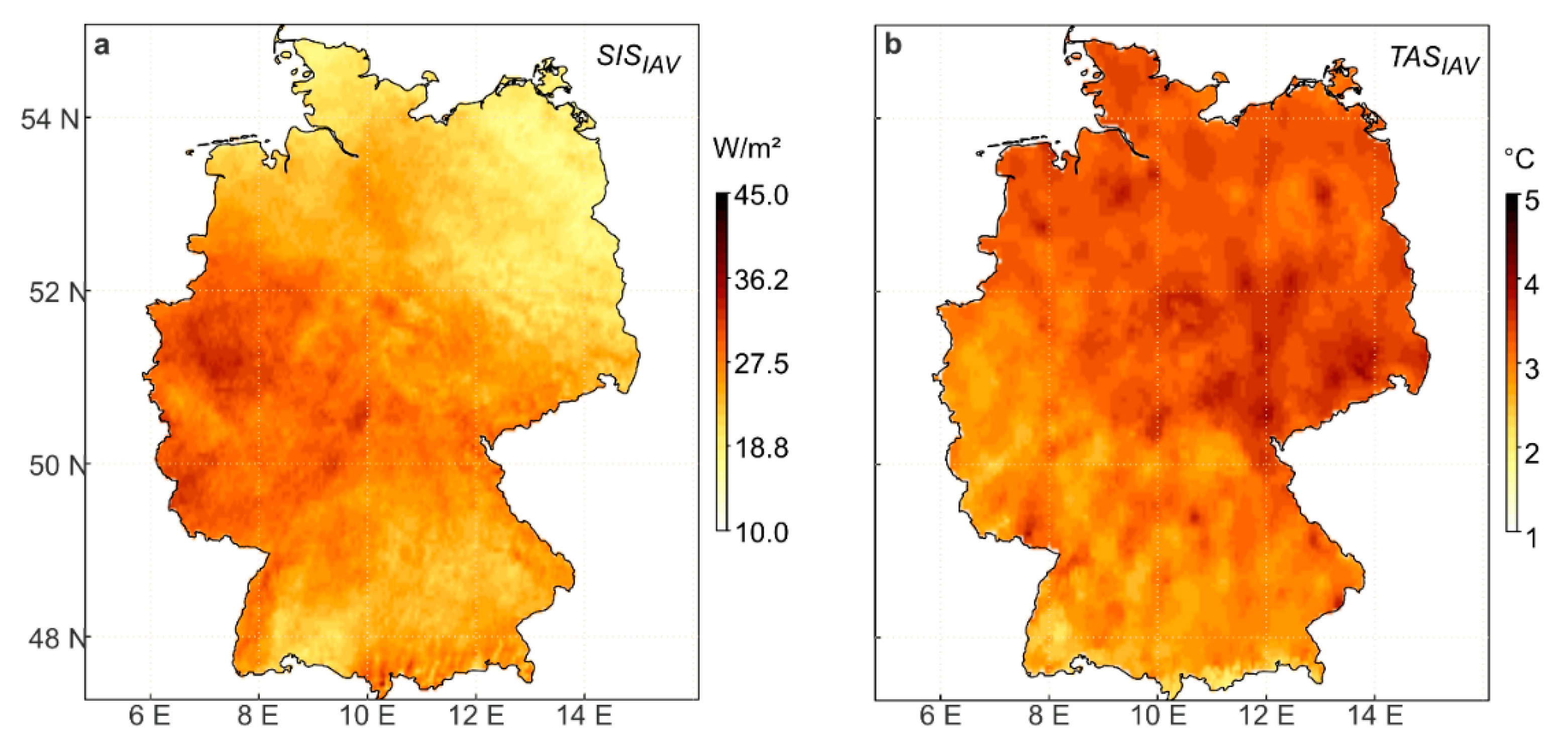
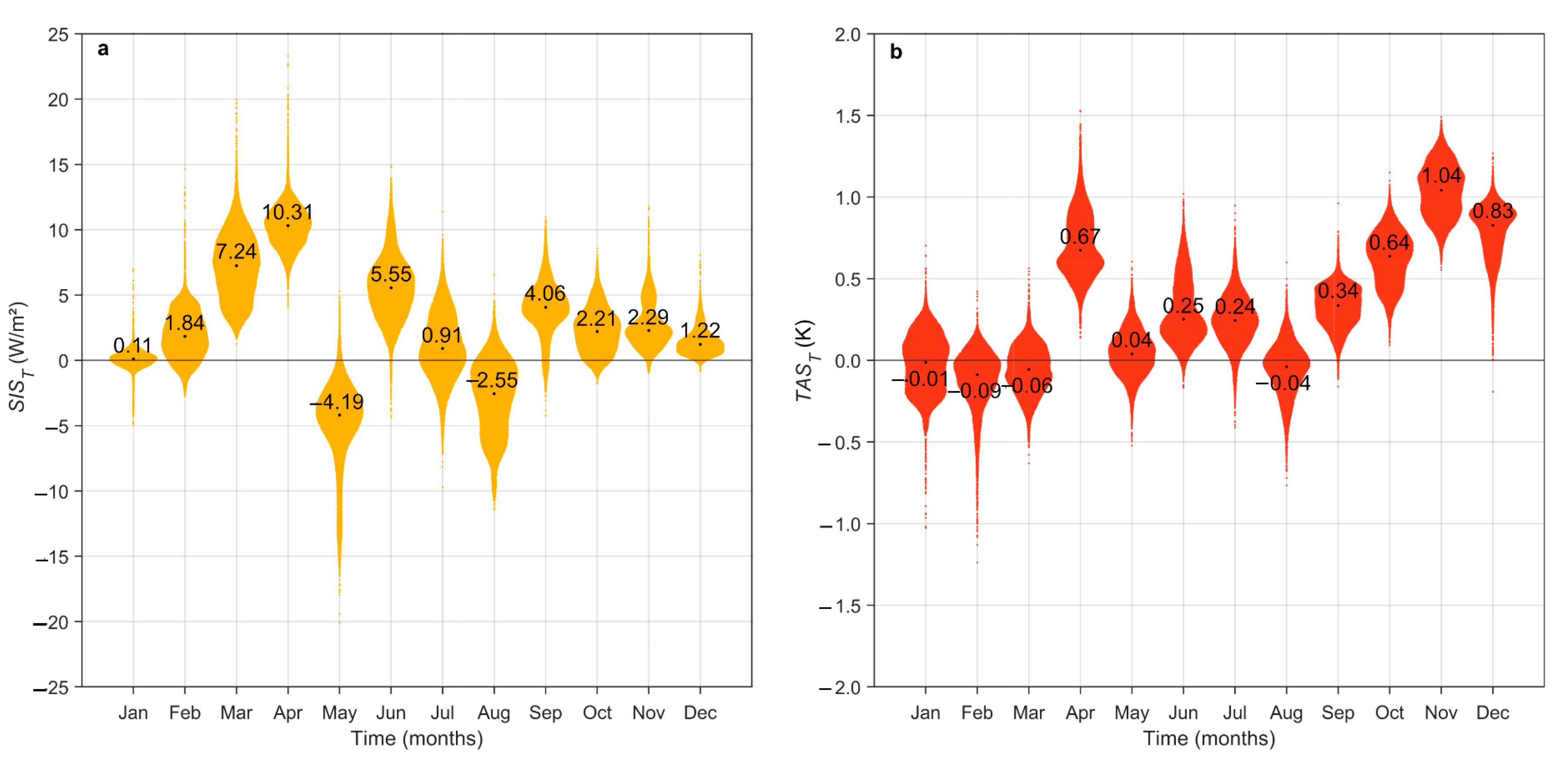
3.2. Trends and Inter-Annual Variability

Different methods of generating electricity require knowledge of the long-term trend of incoming solar energy. For this purpose, the long-term SIS values (SIS_T) were calculated for each grid cell and month for the study period. As a result, Figure 3a shows the monthly frequency distributions of the trends in violin plots. The width of each individual violin is a measure of the frequency of the respective monthly trend. The upward and downward peaks of the violins indicate the extreme values of the monthly trends. The median values of the trends are given as numerical values at the respective black dots.

The monthly SIS_T values show a pronounced seasonal pattern. While local trends cluster around zero in January, they increase in February, March, and especially in April. The median SIS_T values are highest in April at about 10 W/m²/10 yr. A significant decrease occurs in May. For this month, most SIS_T values are negative, and the monthly median is −4.19 W/m²/10 yr, which is the lowest median of the whole year. In the second half of the year, the median monthly values of SIS_T vary between −2.55 and +5.55 W/m²/10 yr. The scattering of the grid cell SIS_T values is small and mainly limited to the range of −10.0 to +10.0 W/m²/10 yr.

The spatial distribution of the SIS variability in the individual months shows a pronounced annual cycle. Here it should be mentioned briefly that SIS_IAV shows a much wider range of variation in all months than SIS_T.

The violin plots for TAS_T shown in Figure 3b were calculated using the same method as those violin plots of SIS_T shown in Figure 3a. The long-term monthly grid cell values of the TAS_T trend also show conspicuous values in two periods of the year (Figure 3b). April shows a noticeable long-term mean increase of TAS_T = 0.8 K/10 yr. From August to December, TAS_T values increase continuously up to 1.0 K/10 yr. For April, another study found similar TAS trend values of 0.5 K/10 yr for the north and 0.2 K/10 yr for the south of Germany [5]. The phenomenon of TAS increase in late summer and early autumn has already been reported earlier [30].

The month with the most pronounced trends in SIS and TAS is April (Figure 4). The most significant increase of SIS_T up to 15 W/m²/10 yr can be seen in Northwestern Germany as well as in Bavaria. The negative trend of cloud fractional cover (CFC_T) in April of −4.1%/10 yr favors this development, further details on CFC_T can be found in Figure 6 and are given in the corresponding text in [20]. From Eastern to Southwestern Germany, an area with a value of SIS_T around 5 W/m²/10 yr is discernible. Again, this behavior can be explained by the variability in CFC.

Regarding TAS_T in April, Germany is divided into two parts: In the northern part there is hardly any trend (<0.5 K/10 yr), while the southern part of Germany shows values up to 1.2 K/10 yr. This is in line with a previous study [5] that found an average trend of TAS in Northern Germany of 0.30 K/10 yr and for Southern Germany of 0.28 K/10 yr for a 65-year period (1951–2015).

This underlines the well-known fact that there has been a significant increase in TAS, especially in the last decade of the study period analyzed by [5]. An increase in TAS can be expected when the NI is positive [31]. In almost all years, the NI values are positive in April.

Since Figure 3 shows the most striking trend in SIS and to some extent also in TAS in spring, the seasonal anomalies of SIS (SIS_MAM) and TAS (TAS_MAM) in spring are shown in Figure 5. Increasing SIS_MAM coincides with an increase in TAS_MAM. In addition to the correlation between SIS_MAM and TAS_MAM, the fluctuations of SIS_MAM and TAS_MAM within the study period were investigated. It was found that large fluctuations of SIS_MAM are associated with large fluctuations of TAS_MAM. For Europe, a correlation coefficient between R = 0.73 and R = 0.86 was found in [2]. Especially for the years from 1990 onwards, the authors calculated high correlation values for the summer months.

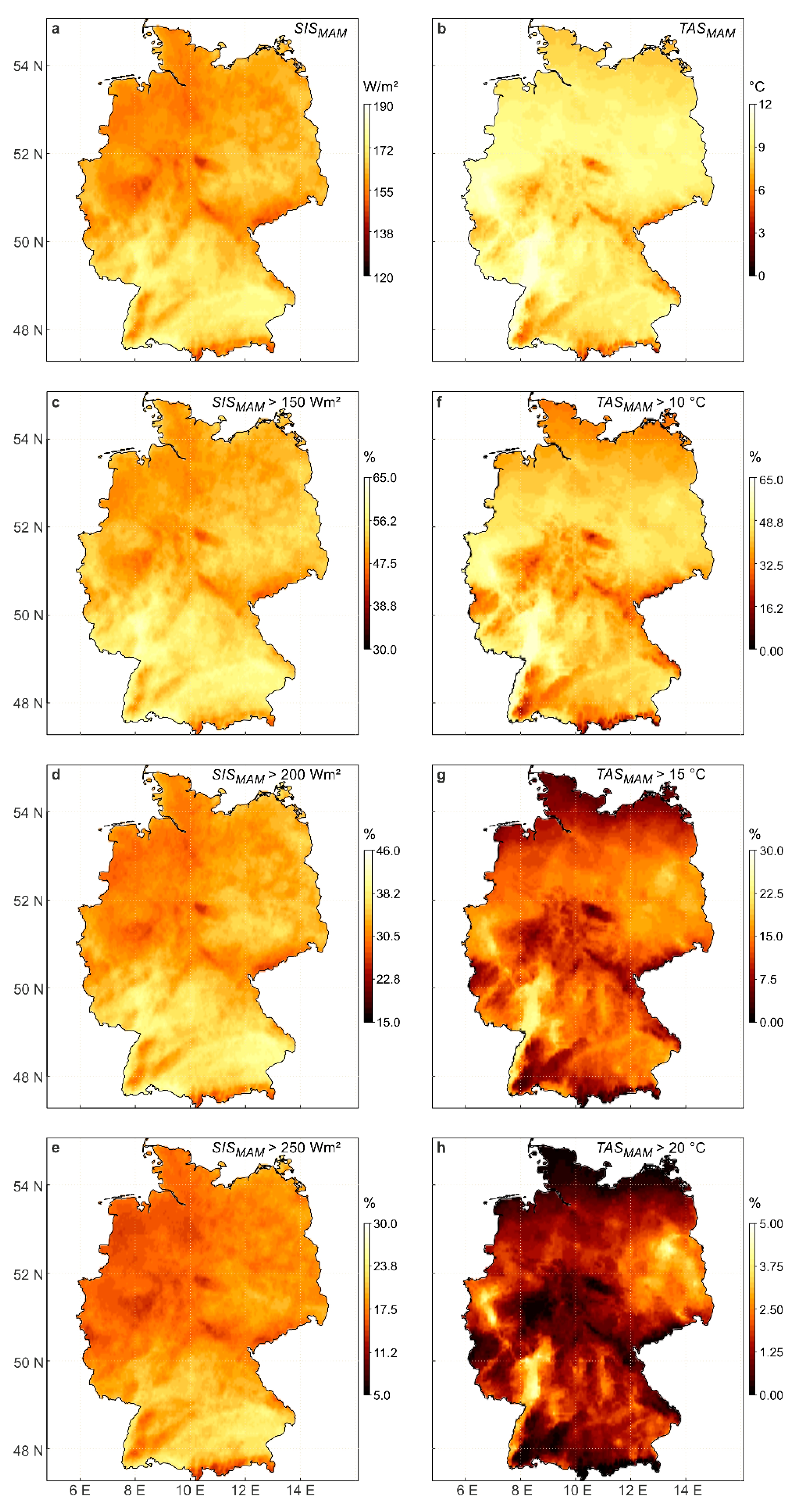
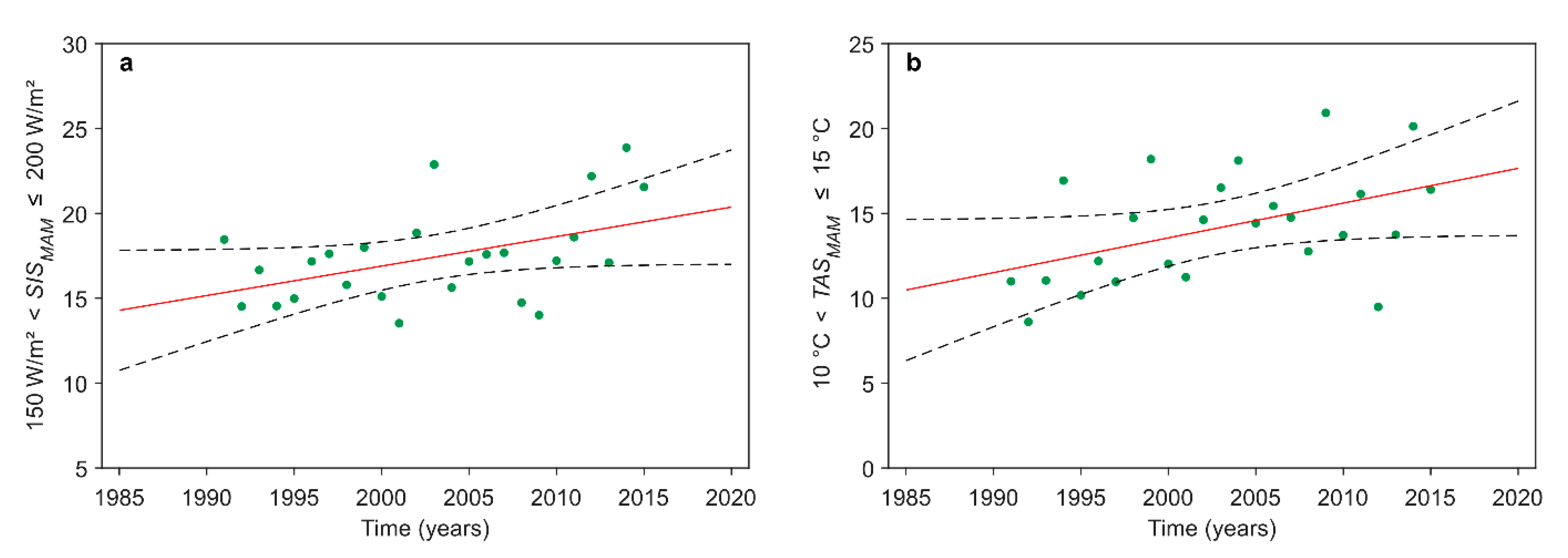
3.3. Changes in High SIS_MAM and TAS_MAM Values

For the dimensioning of PV plants, their operators do not need the long-term means of SIS and TAS, but rather, information on how often the given thresholds are exceeded. Corresponding results are given here.

Since the most significant changes in SIS and TAS are to be expected in spring, Figure 6a displays the spatial patterns of SIS_MAM. In Southern Germany, higher SIS_MAM values are found than in the north. The low mountains in Central Germany are characterized by significantly lower SIS_MAM values.

The long-term means of SIS_MAM are between 120 and 190 W/m². In cases of cloudless sky, the average daily irradiance in the study area may be up to 500 W/m².

Since hardly a significant number of events could be detected above 300 W/m², the number of SIS_MAM values exceeding the thresholds of 150, 200, and 250 W/m² was investigated. Figure 6c–e show the percentage of all cases of SIS_MAM exceeding the thresholds set in the spring months. A limit value of SIS_MAM = 150 W/m² is exceeded in at least 50% of all grid cells in almost the whole of Germany. Raising the threshold to SIS_MAM = 200 W/m² and SIS_MAM = 250 W/m² limits high shares of events to the southern parts of the country.

High TAS_MAM > 10 °C mainly occur in the southwestern and western parts of the study area (Figure 6b). Lower TAS_MAM values of about 5 °C can be observed in the low mountains and the foothills of the Alps. The average mean values of TAS_MAM are between 0 and 12 °C. In the study period the average maximum TAS_MAM = 27 °C. Figure 6f–h show the percentage of all TAS_MAM cases exceeding the thresholds of 10, 15, and 20 °C in the spring months.

In at least 50% of all cells, TAS_MAM = 10 °C is exceeded. The lowlands are marked with 15% and the Rhine Valley with 60% of all the cases. The limit value of TAS_MAM = 15 °C is exceeded in 22% of all cases in the Rhine Valley. In the other areas of Germany, this limit is exceeded in between 5% and 10% of all cases. The limit value of 20 °C is exceeded in only 3% of all cases.

Additional information on the long-term increase of SIS_MAM and TAS_MAM can be obtained by studying the increase in the number of events in individual SIS_MAM and TAS_MAM ranges. Due to the development of solar energy applications over recent years, there is an increasing need to study the transition of SIS_MAM and TAS_MAM to higher levels. Therefore, the long-term change in the number of events in the SIS_MAM range of 150–200 W/m² and in the TAS_MAM range of 10–15 °C is displayed in Figure 7. The trends of SIS_MAM and TAS_MAM significantly increase.

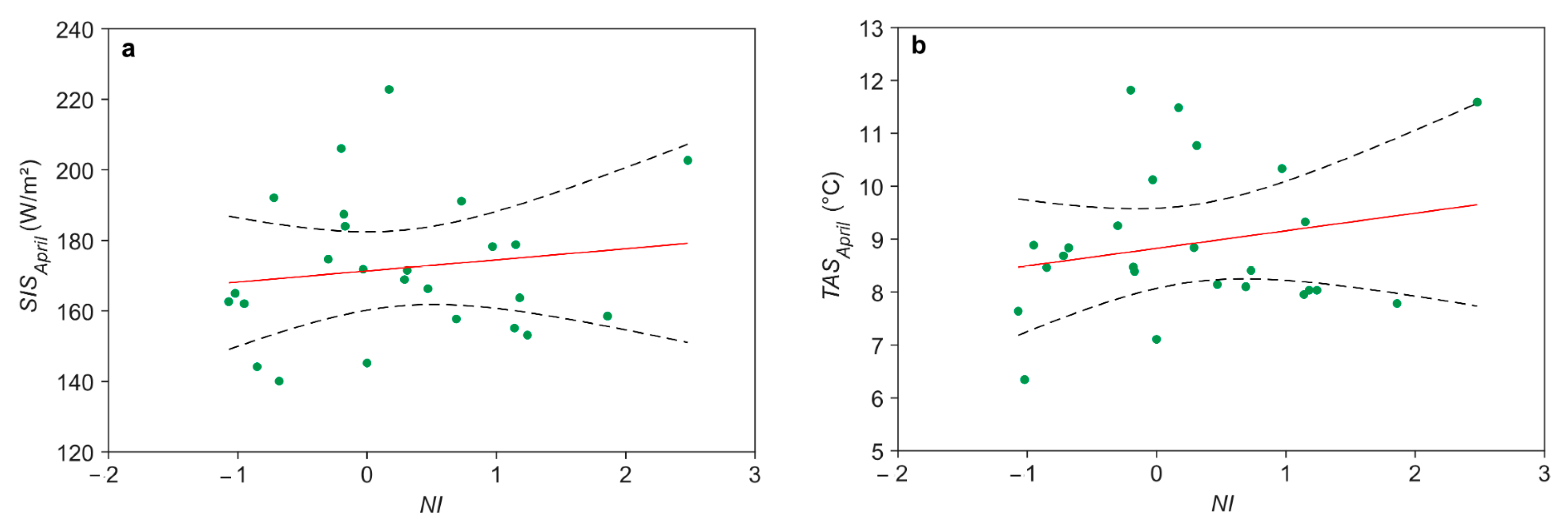
3.4. Influence of the NAO Index on SIS and TAS

As an example, for April, the correlations between NI and SIS (SIS_April) and NI and TAS (TAS_April) are shown in Figure 8.

Both figures show a weak dependence of SIS_April and TAS_April on NI. Similar correlations for all months are given in

Table 2. Correlation coefficients (R) between monthly values of SIS and TAS (R_SIS,TAS), NI and SIS (R_NI,SIS), and NI and TAS (R_NI,TAS) in Germany from 1991–2015. R values on significance level p < 0.05 are in bold.

Month	RSIS,TAS	RNI,SIS	RNI,TAS
January	−0.15	0.14	0.50
February	0.21	0.40	0.43
March	0.33	0.35	0.66
April	0.68	0.15	0.22
May	0.84	0.31	0.34
June	0.74	0.32	0.00
July	0.93	0.38	0.32
August	0.76	0.43	0.29
September	0.74	0.31	0.21
October	0.30	−0.06	0.15
November	0.43	0.35	−0.04
December	0.43	0.21	0.80

.

We found, similar to the study of [6], an interdependence of SIS, TAS, and NI of about 0.40–0.60 for the study area.

With the exception of January, the monthly R_SIS,TAS is positive. In July, which has the longest light days, R_SIS,TAS = 0.93. The correlation from April to September is significant at p < 0.05.

In the winter months, the high and also significant R_NI,TAS values are striking. During this time, TAS is essentially determined by high NI, which is responsible for a pronounced westerly wind circulation. The same was found for the BSRN station Tartu–Tõravere in Estonia [6] which indicates that atmospheric circulation is an important factor controlling TAS in the study areas.

The results in [6] differ slightly from those of our study for several reasons: (1) we used data records from a larger area (48° N–55° N/6° E–15° E) rather than from a single station (BSRN station Tartu–Tõravere in Estonia), (2) the station is located about 5° further north (about 500 km) than the northernmost point of Germany. Thus, in the winter months, the days of light are significantly shorter than those in Germany. In the summer months, the ratio reverses in favor of Tartu-Tõravere. (3) The two study periods are not identical: The author [6] used data records from the period 1955–2007.

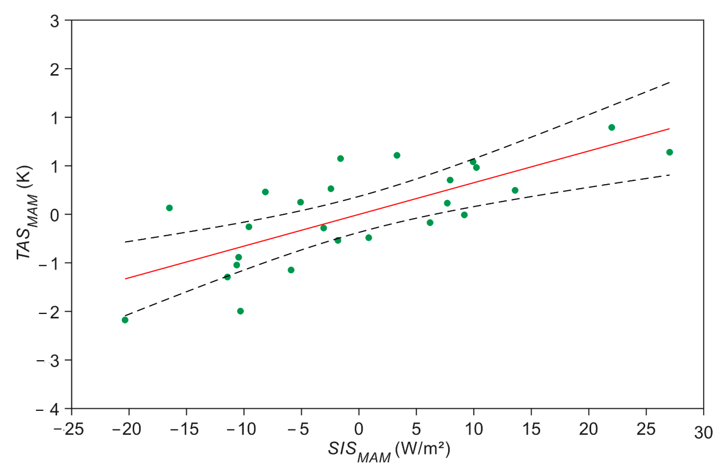
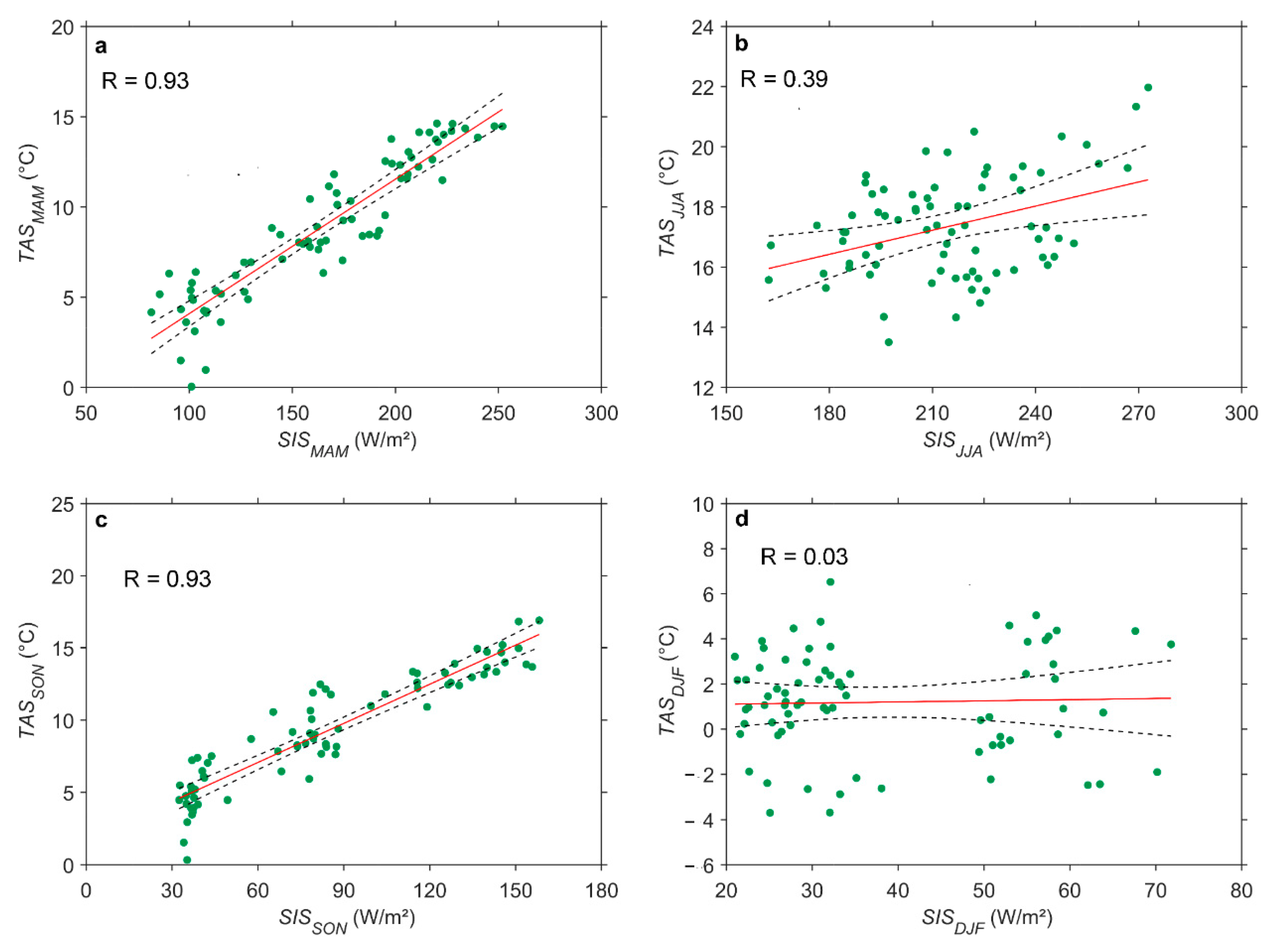
3.5. Correlation between SIS and TAS

The similar long-term increase in SIS and TAS in April and October presented in Figure 3 stimulated a correlation analysis of these two variables. A good correlation between these variables was also found by [3]. Figure 9a–d show the corresponding results for the four seasons. Only in spring and autumn, is a clear dependence of TAS on SIS discernible. The similar increase in these two variables in these two seasons indicates their good correlation.

3.6. Ratio of Temperature and Solar Radiation

Finally, the regional structure of the long-term ratio TAS/SIS in the four seasons is given in Figure 10a–d. In all four seasons, the ratio is between 0 and 0.15 K/W/m². The larger the quotient (light areas), the more TAS reacts on an increase in SIS. This is clearly visible in all four seasons in the large basins in Southwestern Germany. While spring and autumn have hardly any regional structure but a strong correlation, the strong increase in autumn is particularly noticeable in Northern Germany. In winter, the sign of K/W/m² reverses in Southern Germany and in the low mountains, while in the north it remains positive. This regional two-part behavior is also evident from the fact that the correlation between SIS and TAS is unstructured in these seasons. This behavior is determined on the one hand by changes in the NI and the lower inter-annual variability of cloud cover [20].

4. Conclusions

To mitigate climate change, solar energy must play an increasingly important role in today and tomorrow’s global energy supply. Before deciding to install PV systems in a particular area, a thorough analysis of the long-term spatial and temporal trends of solar radiation and surface air temperature is required. The following characteristic parameters of surface incoming solar radiation and surface air temperature are important for PV system operators to optimize their systems: long-term averages in the individual regions, the long-term trend of mean values and their variability, and finally an increase in exceedances of specified thresholds.

For the climate of the study area, we found a simultaneous long-term increase in incoming solar radiation and air temperature in spring. A further increase in surface air temperature was observed in autumn. The annual variability of incoming solar radiation and surface air temperature is much greater than their long-term variability.

Although an increase in solar radiation does not directly result in an increase in surface air temperature, an influence of solar radiation on surface air temperature was shown.

It was found that the TAS/SIS ratio is always positive, except in winter. This indicates a slight but almost equal interdependence of the two variables in the whole study area. Due to the short period of light days in winter, the ratios are unclear in this season.

The variable input of solar radiation in the study area influences the large-scale circulation, expressed by the variability of the NAO index. This quantity then controls the change in surface air temperature. These interdependencies are responsible for the efficiency of the PV systems and must therefore be considered by the operators of PV systems.

References

1. Obregón, M.A.; Costa, M.J.; Silva, A.M.; Serrano, A. Spatial and temporal variation of aerosol and water vapour effects on solar radiation in the Mediterranean basin during the last two decades. Remote Sens. 2020, 12, 1316. [Google Scholar] [CrossRef]
2. Wang, K.; Dickinson, R.E. Contribution of solar radiation to decadal temperature variability over land. Proc. Natl. Acad. Sci. USA 2013, 110, 14877–14882. [Google Scholar] [CrossRef] [PubMed]
3. Reitan, C.H. A Climatic model of solar radiation and temperature change. Quat. Res. 1974, 4, 25–38. [Google Scholar] [CrossRef]
4. Yang, C.; Yan, Z.; Jones, P.D.; Davies, T.D.; Moberg, A.; Bergström, H.; Camuffo, D.; Cocheo, C.; Maugeri, M.; Demarée, G.R.; et al. Trends of extreme temperatures in Europe and China based on daily observations. Clim. Chang. 2002, 53, 355–392. [Google Scholar] [CrossRef]
5. Waldau, T.; Chmielewski, F.M. Spatial and temporal changes of spring temperature, thermal growing season and spring phenology in Germany 1951–2015. Meteorol. Z. 2018, 27, 335–342. [Google Scholar] [CrossRef]
6. Russak, V. Changes in solar radiation and their influence on temperature trend in Estonia (1955–2007). J. Geophys. Res. Atm. 2009, 114, D00D01. [Google Scholar] [CrossRef]
7. Al-Kouz, W.; Al-Dahidi, S.; Hammad, B.; Al-Abed, M. Modeling and analysis framework for investigating the impact of dust and temperature on PV systems’ performance and optimum cleaning frequency. Appl. Sci. 2019, 9, 1397. [Google Scholar] [CrossRef]
8. World Meteorological Organization. Guide to Instruments and Methods of Observation (WMO-No. 8). In Guide to Meteorological Instruments and Methods of Observation; World Meteorological Organization: Geneva, Switzerland, 2018; Volumes I and II. [Google Scholar]
9. Sawadogo, W.; Abiodun, B.J.; Okogbue, E.C. Impacts of global warming on photovoltaic power generation over West Africa. Ren. Energy 2020, 151, 263–277. [Google Scholar] [CrossRef]
10. Kawajiri, K.; Oozeki, T.; Genchi, Y. Effect of temperature on PV potential in the world. Environ. Sci. Technol. 2011, 45, 9030–9035. [Google Scholar] [CrossRef] [PubMed]
11. Hasanuzzaman, M.; Malek, A.B.M.A.; Islam, M.M.; Pandey, A.K.; Rahim, N.A. Global advancement of cooling technologies for PV systems: A review. Sol. Energy 2016, 137, 25–45. [Google Scholar] [CrossRef]
12. Federal Network Agency (Bundesnetzagentur). Download Market Data. Available online: https://www.smard.de/en/downloadcenter/download-market-data (accessed on 1 August 2022).
13. van der Wiel, K.; Stoop, L.P.; van Zuijlen, B.R.H.; Blackport, R.; van den Broek, M.A.; Selten, F.M. Meteorological conditions leading to extreme low variable renewable energy production and extreme high energy shortfall. Renew. Sustain. Energy Rev. 2019, 111, 261–275. [Google Scholar] [CrossRef]
14. Schindler, D.; Behr, H.D.; Jung, C. On the spatiotemporal variability and potential of complementarity of wind and solar resources. Energy Convers. Manag. 2020, 218, 113016. [Google Scholar] [CrossRef]
15. IPCC. Sixth Assessment Report (AR6) 2021/2022. Available online: https://www.ipcc.ch/assessment-report/ar6/ (accessed on 9 June 2022).
16. National Oceanic and Atmospheric Administration. Indices and Forecasts, NAO (North Atlantic Oscillation). Available online: https://www.cpc.ncep.noaa.gov/products/precip/CWlink/daily_ao_index/teleconnections.shtml (accessed on 9 June 2022).
17. Kothe, S.; Hollmann, R.; Pfeifroth, U.; Träger-Chatterjee, C.; Trentmann, J. The CM SAF R Toolbox—A tool for the easy usage of satellite-based climate data in NetCDF format. ISPRS Int. J. Geo-Inf. 2019, 8, 109. [Google Scholar] [CrossRef]
18. Pfeifroth, U.; Kothe, S.; Trentmann, J.; Hollmann, R.; Fuchs, P.; Kaiser, J.; Werscheck, M. Surface Radiation Data Set—Heliosat (SARAH), ed. 2.1; Satellite Application Facility on Climate Monitoring (CM SAF): Offenbach am Main, Germany, 2019. [Google Scholar] [CrossRef]
19. Müller, R.; Pfeifroth, U.; Träger-Chatterjee, C.; Trentmann, J.; Cremer, R. Digging the METEOSAT treasure-3 decades of solar surface radiation. Remote Sens. 2015, 7, 8067–8101. [Google Scholar] [CrossRef]
20. Behr, H.D.; Jung, C.; Trentmann, J.; Schindler, D. Using satellite data for assessing spatiotemporal variability and complementarity of solar resources—A case study from Germany. Meteorol. Z. 2021, 30, 515–532. [Google Scholar] [CrossRef]
21. Frick, C.; Steiner, H.; Mazurkiewicz, A.; Riediger, U.; Rauthe, M.; Reich, T.; Gratzki, A. Central European high-resolution gridded daily data sets (HYRAS): Mean temperature and relative humidity. Meteorol. Z. 2014, 23, 15–32. [Google Scholar] [CrossRef]
22. Mann, H.B. Nonparametric Tests against Trend. Econometrica 1945, 13, 245–259. [Google Scholar] [CrossRef]
23. Jung, C.; Schindler, D. On the inter-annual variability of wind energy generation—A case study from Germany. Appl. Energy 2018, 230, 845–854. [Google Scholar] [CrossRef]
24. Kasten, F.; Czeplak, G. Solar and terrestrial radiation dependent on the amount and type of cloud. Sol. Energy 1980, 24, 177–189. [Google Scholar] [CrossRef]
25. Hurrel, J.W.; Kushnir, Y.; Ottersen, G.; Visbeck, M. The North Atlantic Oscillation: Climatic Significance and Environmental Impact; Geophysical Monograph Series; American Geophysical Union: Washington, DC, USA, 2003; Volume 134. [Google Scholar] [CrossRef]
26. Pfeifroth, U.; Bojanowski, J.S.; Clerbaux, N.; Manara, V.; Sanchez-Lorenzo, A.; Trentmann, J.; Walawender, J.P.; Hollmann, R. Satellite-based trends of solar radiation and cloud parameters in Europe. Adv. Sci. Res. 2018, 15, 31–37. [Google Scholar] [CrossRef]
27. Huld, T.; Trentmann, J. Variability and trend in the annual solar irradiation determined from METEOSAT satellite data. In Proceedings of the 31st EUPVSEC, Hamburg, Germany, 14–18 September 2015; pp. 2073–2076. [Google Scholar] [CrossRef]
28. Alexandri, G.; Georgoulias, A.K.; Meleti, C.; Balis, D.; Kourtidis, K.A.; Sanchez-Lorenzo, A.; Trentmann, J.; Zanis, P. A high resolution satellite view of surface solar radiation over the climatically sensitive region of Eastern Mediterranean. Atmos. Res. 2017, 188, 107–121. [Google Scholar] [CrossRef]
29. Manara, V.; Bassi, M.; Brunetti, M.; Cagnazzi, B.; Maugeri, M. 1990–2016 surface solar radiation variability and trend over the Piedmont region (northwest Italy). Theor. App. Clim. 2019, 136, 849–862. [Google Scholar] [CrossRef]
30. Mäder, C.; Richter, S.; Lehmann, H. Globale Erwärmung im letzten Jahrzehnt? Umweltbundesamt, 2013. Available online: https://www.umweltbundesamt.de/themen/globale-erwaermung-im-letzten-jahrzehnt (accessed on 9 June 2022).
31. van der Wiel, K.; Bloomfield, H.C.; Lee, R.W.; Stoop, L.P.; Blackport, R.; Screen, J.A.; Selten, F.M. The influence of weather regimes on European renewable energy production and demand. Environ. Res. Lett. 2019, 14, 094010. [Google Scholar] [CrossRef]
Figure 1. Mean values of (a) SIS (SISP), (b) TAS (TASP) at the grid cells in 1991–2015, trends of annual mean values of (c) solar radiation SISA (SIST = 2.4 W/m2/10 yr, R2 = 0.13), and (d) surface air temperature TASA (TAST = 0.32 K/10 yr, R2 = 0.12) in Germany. The black dashed lines indicate the 95% confidence intervals for the regression models.
Meteorology 01 00022 g001
Figure 2. Inter-annual variability of annual means of (a) surface incoming solar radiation (SISIAV) and (b) air temperature (TASIAV) in Germany in 1991–2015.
Meteorology 01 00022 g002
Figure 3. Violin plots of 10-year trend values of monthly (a) surface incoming solar radiation (SIST), and (b) air temperature (TAST) in Germany from 1991–2015 at the grid cells. The black dots mark the medians, which are given as numerical values.
Meteorology 01 00022 g003
Figure 4. Ten-year trends of (a) SIS (SIST) and (b) TAS (TAST) in April in Germany from 1991–2015.
Meteorology 01 00022 g004
Figure 5. Anomalies of TAS (TASMAM) as a function of anomalies of SIS (SISMAM) in spring (MAM) in Germany from 1991–2015 with a root mean square error RMSE = 0.71 and R2 = 0.55. The black dashed lines indicate the 95% confidence intervals for the regression model.
Meteorology 01 00022 g005
Figure 6. Seasonal means of (a) SIS (SISMAM) and (b) TAS (TASMAM) in spring (MAM). Share of events where SISMAM or TASMAM at each grid point is greater than (c) 150, (d) 200, (e) 250 W/m2, and (f) 10, (g) 15, (h) 20 °C in Germany from 1991–2015.
Meteorology 01 00022 g006
Figure 7. Long-term change in (a) solar radiation (SISMAM) in the range 150 W/m2 < SISMAM ≤ 200 W/m2 (1.73 W/m2/10 yr and R2 = 0.22) and (b) surface air temperature (TASMAM) in the range 10 °C < TASMAM ≤ 15 °C (2.1 °C/10 yr and R2 = 0.21) in spring (MAM) in Germany from 1991–2015. The black dashed lines indicate the 95% confidence intervals for the regression model.
Meteorology 01 00022 g007
Figure 8. Change in (a) SISAprilNISISApril = 3.16, R N I , S I S 2 = 0.021) and (b) TASAprilNITASApril = 0.33, R N I , T A S 2 = 0.05) in dependence on the NAO index (NI) in April in Germany 1991–2015. The black dashed lines indicate the 95% confidence intervals for the regression model.
Meteorology 01 00022 g008
Figure 9. Correlation of seasonal means of SIS and TAS in (a) spring (MAM), (b) summer (JJA), (c) autumn (SON), and (d) winter (DJF) in Germany from 1991–2015. The correlation coefficient (R) is given for each season in the corresponding figure. The black dashed lines indicate the 95% confidence intervals for the regression model.
Figure 10. Ratio of surface air temperature (TAS) and solar radiation (SIS) in (a) spring (MAM), (b) summer (JJA), (c) autumn (SON), and (d) winter (DJF) in Germany 1991–2015.
Meteorology 01 00022 g009