
Development and Investigation of a Separation Process Within Cross-Flow with Superimposed Electric Field


Abstract
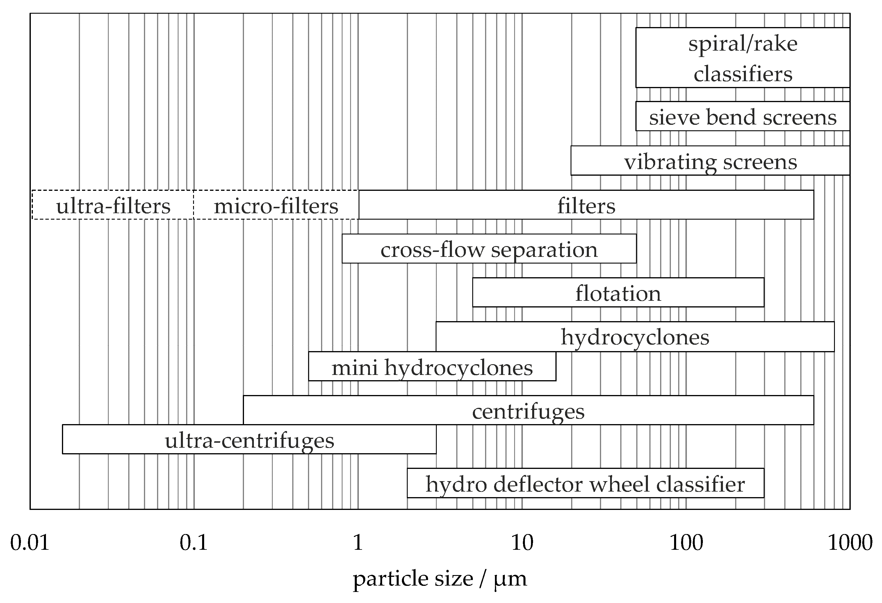
1. Introduction
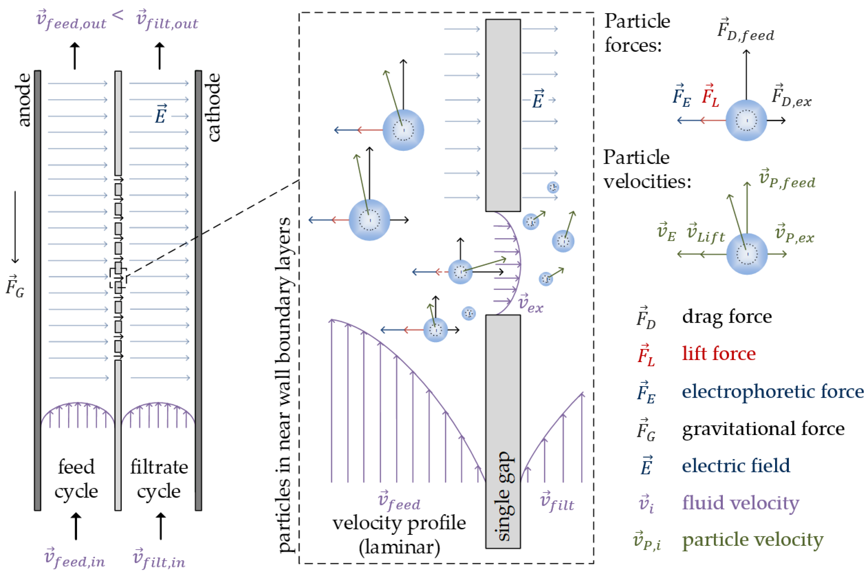
2. Separation Method and Mechanisms
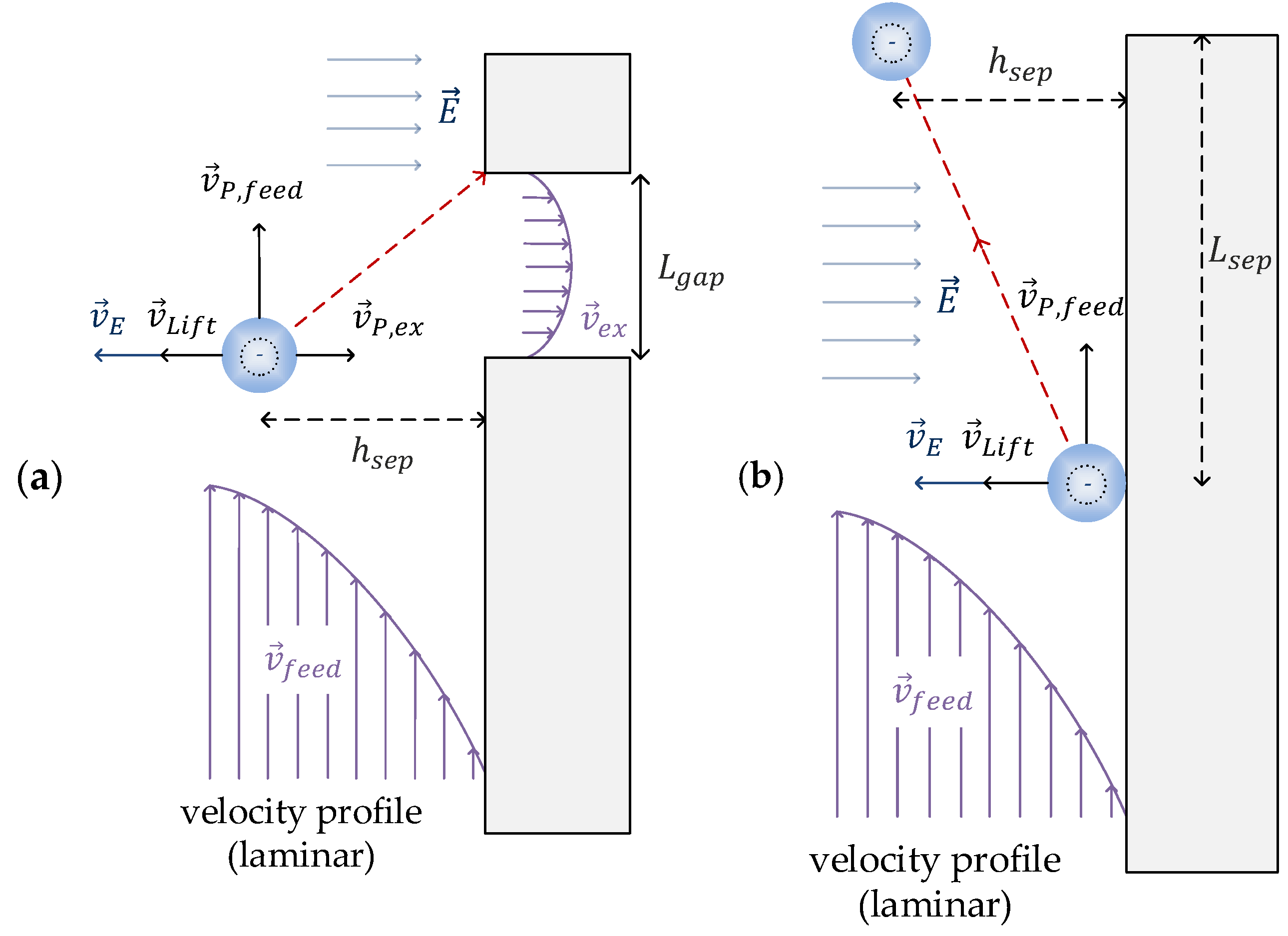
2.1. Hydrodynamic Forces
2.2. Electrophoretic Forces
2.3. Calculation of a Theoretical Separation with a Balance of Forces
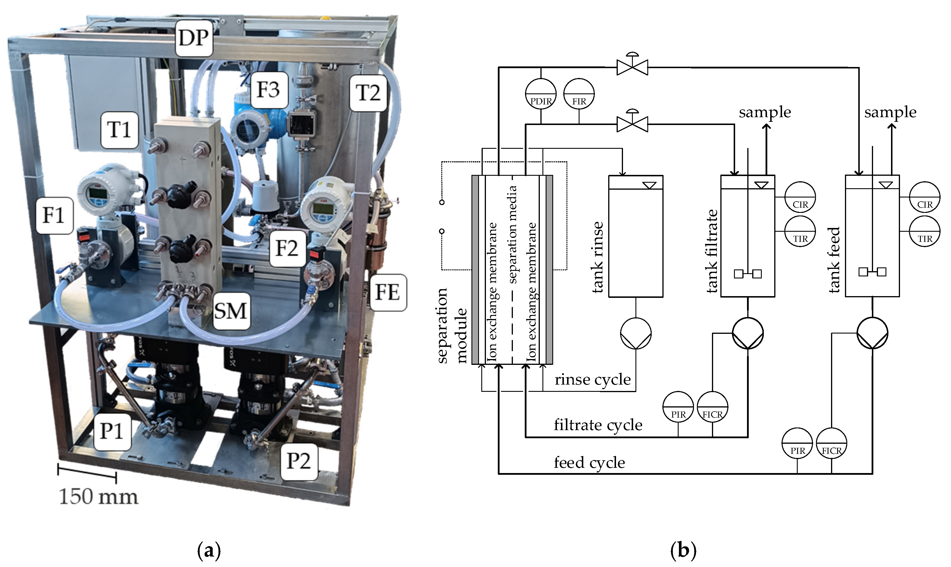
3. Experimental Setup, Simulation Parameters and Materials
3.1. Experimental Setup
3.2. Modelling of the Multidimensional Separation
3.3. Particle System
4. Results
4.1. Investigation of the Particle Motion in the Discontinuous Process
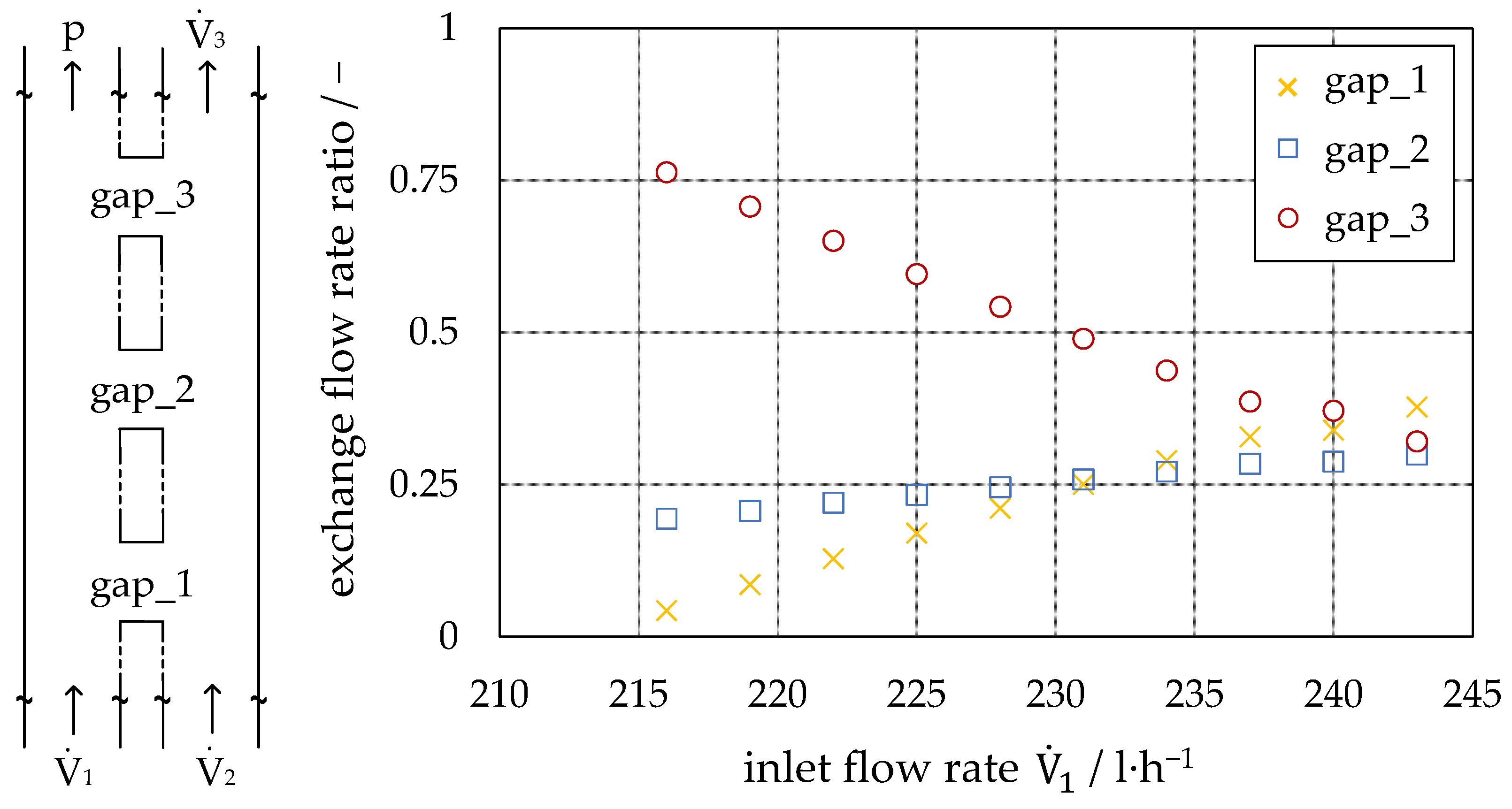
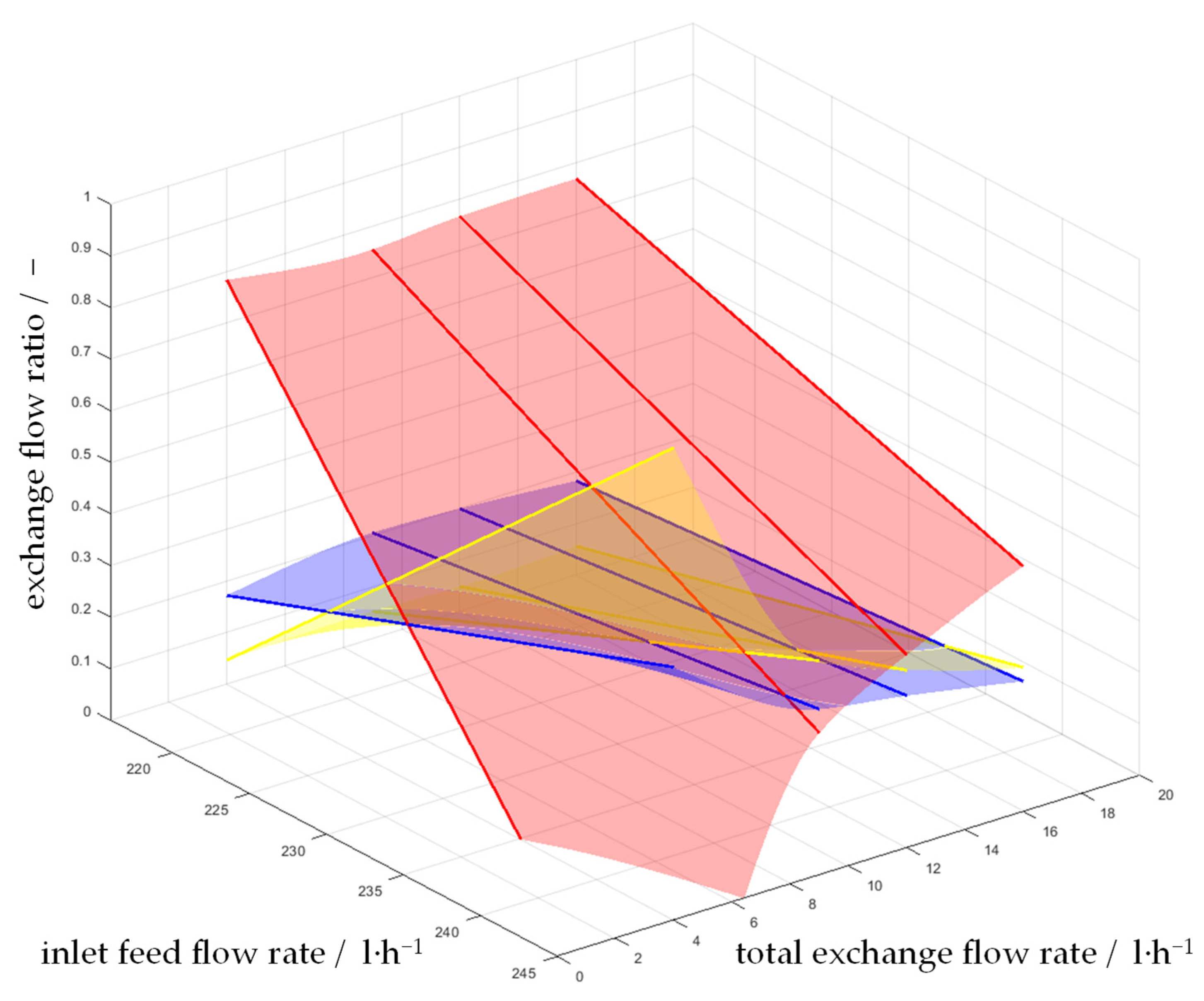
4.2. Investigation on Continuous Separation with Scale-Up Approaches
5. Conclusions
Author Contributions
Funding
Data Availability Statement
Acknowledgments
Conflicts of Interest
Abbreviations
| CFD | computational fluid dynamics |
| DC | direct current |
| DI | deionized |
| DLS | dynamic light scattering |
| EP | electrophoresis |
| EPM | electrophoretic mobility |
| EO | electro-osmosis |
| PSD | particle size distribution |
| SLS | static light scattering |
| UDF | user defined function |
References
- Steigerwald, J.M. Chemical Mechanical Planarization of Microelectronic Materials; John Wiley: New York, NY, USA, 1997. [Google Scholar]
- Bitsch, B.; Willenbacher, N.; Wenzel, V.; Schmelzle, S.; Nirschl, H. Einflüsse der mechanischen Verfahrenstechnik auf die Herstellung von Elektroden für Lithium-Ionen-Batterien. Chem. Ing. Tech. 2015, 87, 466–474. [Google Scholar] [CrossRef]
- Oosterbeek, R.N.; Zhang, X.C.; Best, S.M.; Cameron, R.E. A technique for improving dispersion within polymer-glass composites using polymer precipitation. J. Mech. Behav. Biomed. Mater. 2021, 123, 104767. [Google Scholar] [CrossRef] [PubMed]
- Tripathy, S.K.; Bhoja, S.K.; Raghu Kumar, C.; Suresh, N. A short review on hydraulic classification and its development in mineral industry. Powder Technol. 2015, 270, 205–220. [Google Scholar] [CrossRef]
- Sygusch, J.; Rudolph, M. Multidimensional Characterization and Separation of Ultrafine Particles: Insights and Advances by Means of Froth Flotation. Powders 2024, 3, 460–481. [Google Scholar] [CrossRef]
- Damm, C.; Long, D.; Walter, J.; Peukert, W. Size and Shape Selective Classification of Nanoparticles. Powders 2024, 3, 255–279. [Google Scholar] [CrossRef]
- Reinecke, S.R.; Zhang, Z.; Blahout, S.; Radecki-Mundinger, E.; Hussong, J.; Kruggel-Emden, H. Investigation of Multidimensional Fractionation in Microchannels Combining a Numerical DEM-LBM Approach with Optical Measurements. Powders 2024, 3, 305–323. [Google Scholar] [CrossRef]
- Müller, F. Wet Classification in the Fines Range < 10 μm. Chem. Eng. Technol. 2010, 33, 1419–1426. [Google Scholar] [CrossRef]
- Ripperger, S. Mikro- und Ultrafiltration mit Membranen; Wiley: Hoboken, NJ, USA, 2023. [Google Scholar]
- Wang, W.K. (Ed.) Membrane Separations in Biotechnology; Biotechnology and Bioprocessing Series No. 26; CRC Press Taylor & Francis Group: Boca Raton, FL, USA, 2019. [Google Scholar]
- Heiskanen, K. Developments in wet classifiers. Int. J. Miner. Process. 1996, 44–45, 29–42. [Google Scholar] [CrossRef]
- Weirauch, L.; Giesler, J.; Pesch, G.R.; Baune, M.; Thöming, J. Highly Permeable, Electrically Switchable Filter for Multidimensional Sorting of Suspended Particles. Powders 2024, 3, 574–593. [Google Scholar] [CrossRef]
- Giesler, J.; Weirauch, L.; Thöming, J.; Pesch, G.R.; Baune, M. Dielectrophoretic Particle Chromatography: From Batch Processing to Semi-Continuous High-Throughput Separation. Powders 2024, 3, 54–64. [Google Scholar] [CrossRef]
- Rhein, F.; Zhai, O.; Schmid, E.; Nirschl, H. Multidimensional Separation by Magnetic Seeded Filtration: Experimental Studies. Powders 2023, 2, 588–606. [Google Scholar] [CrossRef]
- Buchwald, T.; Schach, E.; Peuker, U.A. A framework for the description of multidimensional particle separation processes. Powder Technol. 2024, 433, 119165. [Google Scholar] [CrossRef]
- Premaratne, W.A.P.J.; Rowson, N.A. Development of a Magnetic Hydrocyclone Separation for the Recovery of Titanium From Beach Sands. Phys. Sep. Sci. Eng. 2003, 12, 215–222. [Google Scholar] [CrossRef]
- Bourgeois, F.; Majumder, A.K. Is the fish-hook effect in hydrocyclones a real phenomenon? Powder Technol. 2013, 237, 367–375. [Google Scholar] [CrossRef]
- Yamamoto, T.; Oshikawa, T.; Yoshida, H.; Fukui, K. Improvement of particle separation performance by new type hydro cyclone. Sep. Purif. Technol. 2016, 158, 223–229. [Google Scholar] [CrossRef]
- Neesse, T.; Dueck, J.; Schwemmer, H.; Farghaly, M. Using a high pressure hydrocyclone for solids classification in the submicron range. Miner. Eng. 2015, 71, 85–88. [Google Scholar] [CrossRef]
- Yamamoto, T.; Kageyama, T.; Yoshida, H.; Fukui, K. Effect of new blade of centrifugal separator on particle separation performance. Sep. Purif. Technol. 2016, 162, 120–126. [Google Scholar] [CrossRef]
- Konrath, M.; Brenner, A.-K.; Dillner, E.; Nirschl, H. Centrifugal classification of ultrafine particles: Influence of suspension properties and operating parameters on classification sharpness. Sep. Purif. Technol. 2015, 156, 61–70. [Google Scholar] [CrossRef]
- Ives, K.J. The Scientific Basis of Flotation; NATO ASI Series, Series E No. 75; Springer: Dordrecht, The Netherlands, 1983. [Google Scholar]
- Gontijo, C.d.F.; Fornasiero, D.; Ralston, J. The Limits of Fine and Coarse Particle Flotation. Can. J. Chem. Eng. 2007, 85, 739–747. [Google Scholar] [CrossRef]
- Miettinen, T.; Ralston, J.; Fornasiero, D. The limits of fine particle flotation. Miner. Eng. 2010, 23, 420–437. [Google Scholar] [CrossRef]
- Lösch, P.; Antonyuk, S. Selective particle deposition at cross-flow filtration with constant filtrate flux. Powder Technol. 2021, 388, 305–317. [Google Scholar] [CrossRef]
- Lösch, P. Methoden zur Diskontinuierlichen und Kontinuierlichen Hydrodynamischen Klassierung Feinster Partikeln in Einer Querströmung. Dissertation, Schriftenreihe des Lehrstuhls für Mechanische Verfahrenstechnik, Technische Universität Kaiserslautern, Kaiserslautern, Germany, 2021. Band 25. [Google Scholar]
- Altmann, J.; Ripperger, S. Particle deposition and layer formation at the crossflow microfiltration. J. Membr. Sci. 1997, 124, 119–128. [Google Scholar] [CrossRef]
- Lösch, P.; Nikolaus, K.; Antonyuk, S. Fractionating of finest particles using cross-flow separation with superimposed electric field. Sep. Purif. Technol. 2021, 257, 117820. [Google Scholar] [CrossRef]
- Sommerfeld, M.; Wirth, K.-E.; Muschelknautz, U. L3 Zweiphasige Gas-Festkörper-Strömungen. In VDI-Wärmeatlas—Mit 320 Tabellen; VDI-Gesellschaft Verfahrenstechnik und Chemieingenieurwesen, VDI/-Buch; Springer: Berlin/Heidelberg, Germany, 2013; pp. 1359–1412. [Google Scholar]
- Hölzer, A.; Sommerfeld, M. New simple correlation formula for the drag coefficient of non-spherical particles. Powder Technol. 2008, 184, 361–365. [Google Scholar] [CrossRef]
- Grohn, P.; Schaedler, L.; Atxutegi, A.; Heinrich, S.; Antonyuk, S. CFD-DEM Simulation of Superquadric Cylindrical Particles in a Spouted Bed and a Rotor Granulator. Chem. Ing. Tech. 2023, 95, 244–255. [Google Scholar] [CrossRef]
- Deshpande, R.; Antonyuk, S.; Iliev, O. DEM-CFD study of the filter cake formation process due to non-spherical particles. Particuology 2020, 53, 48–57. [Google Scholar] [CrossRef]
- Sommerfeld, M.; Horender, S. Fluid Mechanics. In Ullmann’s Encyclopedia of Industrial Chemistry; Wiley-VCH: Weinheim, Germany, 2012. [Google Scholar] [CrossRef]
- Kaskas, A.A. Schwarmgeschwindigkeiten in Mehrkornsuspensionen am Beispiel der Sedimentation. Doctoral Dissertation, Technische Universität Berlin, Berlin, Germany, 1970. [Google Scholar]
- Morsi, S.A.; Alexander, A.J. An investigation of particle trajectories in two-phase flow systems. J. Fluid Mech. 1972, 55, 193. [Google Scholar] [CrossRef]
- Goossens, W.R. Review of the empirical correlations for the drag coefficient of rigid spheres. Powder Technol. 2019, 352, 350–359. [Google Scholar] [CrossRef]
- Zhang, J.; Yan, S.; Yuan, D.; Alici, G.; Nguyen, N.-T.; Warkiani, M.E.; Li, W. Fundamentals and applications of inertial microfluidics: A review. Lab Chip 2016, 16, 10–34. [Google Scholar] [CrossRef]
- Segré, G.; Silberberg, A. Radial Particle Displacements in Poiseuille Flow of Suspensions. Nature 1961, 189, 209–210. [Google Scholar] [CrossRef]
- Segré, G.; Silberberg, A. Behaviour of macroscopic rigid spheres in Poiseuille flow Part 1. Determination of local concentration by statistical analysis of particle passages through crossed light beams. J. Fluid Mech. 1962, 14, 115–135. [Google Scholar] [CrossRef]
- Segré, G.; Silberberg, A. Behaviour of macroscopic rigid spheres in Poiseuille flow Part 2. Experimental results and interpretation. J. Fluid Mech. 1962, 14, 136–157. [Google Scholar] [CrossRef]
- Ho, B.P.; Leal, L.G. Inertial migration of rigid spheres in two-dimensional unidirectional flows. J. Fluid Mech. 1974, 65, 365–400. [Google Scholar] [CrossRef]
- Saffman, P.G. The lift on a small sphere in a slow shear flow. J. Fluid Mech. 1965, 22, 385–400. [Google Scholar] [CrossRef]
- Lösch, P.; Nikolaus, K.; Antonyuk, S. Classification of Fine Particles Using the Hydrodynamic Forces in the Boundary Layer of a Membrane. Chem. Ing. Tech. 2019, 91, 1656–1662. [Google Scholar] [CrossRef]
- Rubin, G. Widerstands-und Auftriebsbeiwerte von Ruhenden, Kugelförmigen Partikeln in Stationären, Wandnahen, Laminaren Grenzschichten. Doctoral Dissertation, Universität Karlsruhe, Karlsruhe, Germany, 1977. [Google Scholar]
- Leighton, D.; Acrivos, A. The lift on a small sphere touching a plane in the presence of a simple shear flow. ZAMP Z. Angew. Math. Phys. 1985, 36, 174–178. [Google Scholar] [CrossRef]
- Bureau, L.; Coupier, G.; Salez, T. Lift at low Reynolds number. Eur. Phys. J. E Soft Matter 2023, 46, 111. [Google Scholar] [CrossRef]
- Yuan, D.; Zhao, Q.; Yan, S.; Tang, S.-Y.; Alici, G.; Zhang, J.; Li, W. Recent progress of particle migration in viscoelastic fluids. Lab Chip 2018, 18, 551–567. [Google Scholar] [CrossRef]
- Mahian, O.; Kolsi, L.; Amani, M.; Estellé, P.; Ahmadi, G.; Kleinstreuer, C.; Marshall, J.S.; Siavashi, M.; Taylor, R.A.; Niazmand, H.; et al. Recent advances in modeling and simulation of nanofluid flows-Part I: Fundamentals and theory. Phys. Rep. 2019, 790, 1–48. [Google Scholar] [CrossRef]
- Mandø, M.; Rosendahl, L. On the motion of non-spherical particles at high Reynolds number. Powder Technol. 2010, 202, 1–13. [Google Scholar] [CrossRef]
- Shi, P.; Rzehak, R. Lift forces on solid spherical particles in unbounded flows. Chem. Eng. Sci. 2019, 208, 115145. [Google Scholar] [CrossRef]
- Besra, L.; Liu, M. A review on fundamentals and applications of electrophoretic deposition (EPD). Prog. Mater. Sci. 2007, 52, 1–61. [Google Scholar] [CrossRef]
- Barany, S. Electrophoresis in strong electric fields. Adv. Colloid Interface Sci. 2009, 147–148, 36–43. [Google Scholar] [CrossRef] [PubMed]
- Kerner, M.; Schmidt, K.; Hellmann, A.; Schumacher, S.; Pitz, M.; Asbach, C.; Ripperger, S.; Antonyuk, S. Numerical and experimental study of submicron aerosol deposition in electret microfiber nonwovens. J. Aerosol Sci. 2018, 122, 32–44. [Google Scholar] [CrossRef]
- O’Brien, R.W.; White, L.R. Electrophoretic mobility of a spherical colloidal particle. J. Chem. Soc. Faraday Trans. 2 1978, 74, 1607. [Google Scholar] [CrossRef]
- Ohshima, H. Electrophoretic mobility of soft particles. Colloids Surf. A Physicochem. Eng. Asp. 1995, 103, 249–255. [Google Scholar] [CrossRef]
- Heintz, A. Thermodynamik der Mischungen—Mischphasen, Grenzflächen, Reaktionen, Elektrochemie, Äußere Kraftfelder; Springer-Verlag GmbH, Lehrbuch; Springer Spektrum: Berlin/Heidelberg, Germany, 2017. [Google Scholar]
- Ferziger, J.H.; Perić, M. Computational Methods for Fluid Dynamics; Springer: Berlin/Heidelberg, Germany, 2002. [Google Scholar]
- Menter, F.R. Two-equation eddy-viscosity turbulence models for engineering applications. AIAA J. 1994, 32, 1598–1605. [Google Scholar] [CrossRef]
- Li, A.; Ahmadi, G. Dispersion and Deposition of Spherical Particles from Point Sources in a Turbulent Channel Flow. Aerosol Sci. Technol. 1992, 16, 209–226. [Google Scholar] [CrossRef]
- Kruggel-Emden, H.; Simsek, E.; Rickelt, S.; Wirtz, S.; Scherer, V. Review and extension of normal force models for the Discrete Element Method. Powder Technol. 2007, 171, 157–173. [Google Scholar] [CrossRef]
- Krull, F.; Hesse, R.; Breuninger, P.; Antonyuk, S. Impact behaviour of microparticles with microstructured surfaces: Experimental study and DEM simulation. Chem. Eng. Res. Des. 2018, 135, 175–184. [Google Scholar] [CrossRef]
- Puderbach, V.; Schmidt, K.; Antonyuk, S. A Coupled CFD-DEM Model for Resolved Simulation of Filter Cake Formation during Solid-Liquid Separation. Processes 2021, 9, 826. [Google Scholar] [CrossRef]
- Krull, F.; Mathy, J.; Breuninger, P.; Antonyuk, S. Influence of the surface roughness on the collision behavior of fine particles in ambient fluids. Powder Technol. 2021, 392, 58–68. [Google Scholar] [CrossRef]
- Strohner, D.; Antonyuk, S. Experimental and numerical determination of the lubrication force between a spherical particle and a micro-structured surface. Adv. Powder Technol. 2023, 34, 104173. [Google Scholar] [CrossRef]
- Tiwari, P.; Antal, S.P.; Podowski, M.Z. Modeling shear-induced diffusion force in particulate flows. Comput. Fluids 2009, 38, 727–737. [Google Scholar] [CrossRef]
- Kurzweil, P. Angewandte Elektrochemie—Grundlagen, Messtechnik, Elektroanalytik, Energiewandlung, Technische Verfahren, Lehrbuch; Springer: Wiesbaden, Germany, 2020. [Google Scholar]


| Ranges | |||
|---|---|---|---|
| 0.1 ≤ Re ≤ 1 | 0 | 24 | 0 |
| 1 < Re ≤ 10 | 3.69 | 22.73 | 0.0903 |
| 10 < Re ≤ 100 | 1.222 | 29.1667 | −3.8889 |
| 100 < Re ≤ 1000 | 0.6167 | 46.5 | −116.67 |
| 1000 < Re ≤ 5000 | 0.3644 | 98.33 | −2778 |
| 5000 < Re ≤ 10,000 | 0.357 | 148.62 | −47,500 |
| Re > 10,000 | 0.46 | 578.7 | −166,200 |
| Unit | Setup No. 1 | |||
|---|---|---|---|---|
| Single-Gap Profile | Three-Gap Profile | |||
| Total length | mm | 420 | ||
| Gap distance | mm | 74.5 | ||
| Main length | mm | 306 | ||
| Main width | mm | 3; 6 | ||
| Main depth | mm | 60 | ||
| In- and Outlet length | ; | mm | 58 | |
| In- and Outlet depth | ; | mm | 22 | |
| Unit | Setup No. 2 | Setup No. 3 | ||
|---|---|---|---|---|
| Enclosed | Optical Accessible | |||
| Total length | mm | 210 | 110 | |
| Main length | mm | 170 | 90 | |
| Main width | mm | 3 | 3 | |
| Main depth | mm | 1 | 1 | |
| In- and Outlet length | mm | 20 | 10 | |
| In- and Outlet depth | mm | 1 | 1 |
| Particle Diameter | 1 µm | 5 µm | 10 µm | 15 µm | 20 µm | |
|---|---|---|---|---|---|---|
| Material | Flow Rate | Initial Wall Distances [µm] Ratio of Horizontal to Vertical Path [µm·mm−1] | ||||
| polystyrene | 5 mL·min−1 | 189.81 0.0077 | 189.38 0.008 | 189.04 0.0106 | 189.53 0.0174 | 191.29 0.0304 |
| 30 mL·min−1 | 150.62 0.0864 | 149.54 0.0858 | 149.75 0.0859 | 149.29 0.0865 | 150.49 0.0896 | |
| d10/µm | d50/µm | d90/µm | d99/µm | wt.% Filtrate/g·L−1 | |
|---|---|---|---|---|---|
| single-gap | ~5 | ~10 | ~16 | ~26 | ~0.55 |
| three-gap | ~7 | ~15 | ~30 | ~45 | ~0.93 |
Disclaimer/Publisher’s Note: The statements, opinions and data contained in all publications are solely those of the individual author(s) and contributor(s) and not of MDPI and/or the editor(s). MDPI and/or the editor(s) disclaim responsibility for any injury to people or property resulting from any ideas, methods, instructions or products referred to in the content. |
© 2025 by the authors. Licensee MDPI, Basel, Switzerland. This article is an open access article distributed under the terms and conditions of the Creative Commons Attribution (CC BY) license (https://creativecommons.org/licenses/by/4.0/).
Share and Cite
Paas, S.; Nikolaus, K.; Antonyuk, S. Development and Investigation of a Separation Process Within Cross-Flow with Superimposed Electric Field. Powders 2025, 4, 6. https://doi.org/10.3390/powders4010006
Paas S, Nikolaus K, Antonyuk S. Development and Investigation of a Separation Process Within Cross-Flow with Superimposed Electric Field. Powders. 2025; 4(1):6. https://doi.org/10.3390/powders4010006
Chicago/Turabian StylePaas, Simon, Kai Nikolaus, and Sergiy Antonyuk. 2025. "Development and Investigation of a Separation Process Within Cross-Flow with Superimposed Electric Field" Powders 4, no. 1: 6. https://doi.org/10.3390/powders4010006
APA StylePaas, S., Nikolaus, K., & Antonyuk, S. (2025). Development and Investigation of a Separation Process Within Cross-Flow with Superimposed Electric Field. Powders, 4(1), 6. https://doi.org/10.3390/powders4010006