Three-Dimensional Particle-Discrete Datasets: Enabling Multidimensional Particle System Characterization Using X-Ray Tomography

Abstract

This collection of studies, conducted within the framework of the DFG-funded Priority Program SPP 2045, explores the role of X-ray tomography in advancing the multidimensional characterization of particulate systems, with a strong focus on enhancing 3D particle-discrete data quality. It critically assesses the limitations of traditional particle characterization methods, particularly those reliant on imaging techniques, and demonstrates how advanced methodologies can overcome these constraints by providing highly detailed and accurate geometric and structural 3D data. The research further introduces innovative sample preparation techniques for particle collectives, aiming to reduce post-processing efforts in image analysis. Additionally, the development of a particle database, aligned with FAIR data principles (Findable, Accessible, Interoperable, and Reusable), supports data sharing and collaborative research. Ultimately, this collection underscores the transformative potential of 3D particle-discrete datasets acquired through X-ray tomography in advancing particle technology and improving particle system analyses across diverse scientific and industrial fields.

1. Introduction

This publication of the Topical Collection Multidimensional Particle Properties: Characterization, Description, Separation is part of the DFG-funded Priority Program SPP 2045 and summarizes the work on three-dimensional particle characterization within the central characterization subproject. The focus is on the particle-discrete description of the 3D particle data, which is not fundamentally new within the computed tomography and image analysis community, but in our opinion is underrepresented in the process-related particle characterization community and requires further motivation. In the following, we therefore focus on the motivation behind the topic and show how these data can serve as the basis for multidimensional property correlations. In the individual sections, we focus on how the quality of the resulting image data is affected and explore ways to maximize it in order to create reliable datasets suitable for multidimensional particle analysis. Application examples are briefly outlined and further considered, but are described in detail in the project-related publications.

The structure of the document is as follows. In the Introduction we will start with an extended motivation on the topic of particle-discrete data. Initially, this might seem trivial and basic, but in many personal discussions it has become evident that the understanding of the importance of particle-discrete data is the essential starting point for better and more comprehensive insight on the multidimensional nature of modern particle-related processes. In this context, multidimensional means considering multiple particle characteristics—like size and shape or size and composition—simultaneously and interdependently, rather than evaluating each characteristic separately, to describe a process such as a separation process. Such analysis we call multidimensional—in this example, a two dimensional one. The Materials and Methods section is divided into two parts. The first will introduce X-ray tomography as a key technique for 3D particle-discrete analysis and the second focuses on how an adapted particle sample preparation technique can significantly support those types of analysis. Please note that in the first two sections, we emphasize the impact on the final quantitative analysis of particle-discrete datasets. The Results and Discussion section is divided into a short description of possible workflows. One workflow comprises multiple particle size scales, the other acquires additional information from different analyses, thereby supplementing tomographic measurements, the so-called correlative workflow. The second part of the section deals with further challenges and future directions.

1.1. The Need for 3D Particle-Discrete Data

When characterizing particulate systems, one can generally distinguish between three different approaches. The first is aggregated parameters, such as characteristic quantiles of a distribution ($x_{10}$, $x_{50}$, $x_{90}$), mean value and variance. The second is class-based, i.e., the proportion of particles in a collective that lies between fixed class boundaries, e.g., a lower and upper particle size. And the third is the acquisition of values for each individual particle, which we refer to hereafter as particle-discrete. In the following, we will see that this ordering is historically due to the low availability of suitable measurement technology. Nowadays, 2D and 3D imaging in particular is able to provide particle-discrete data from which one can easily derive class-based and aggregated representations, be it for condensing information or for comparison with other measurement methods.

Individual measurement techniques are more or less “optimized” for one specific particle characteristic, in many cases equivalent quantities such as the scattered light equivalent diameter, e.g., in case of laser diffraction [1]; the equivalent hydrodynamic diameter, e.g., in case of an ultracentrifuge [2]; or the projection equivalent diameter, e.g., in case of sieving [3]. First, laser diffraction is currently the standard method for particle characterization in the particle size range from 1 $\mu$$\mathrm{m}$ to approx. 1000 $\mu$$\mathrm{m}$. The fact that the calculated software output of the laser diffraction measurement is given by the system as a number-based or volume-weighted distribution of particle size suggests a particle-discrete dataset. But actually, this is not the case. While moving through the measurement volume within the laser beam, the interaction of a set of particles and the incoming laser photons creates a diffraction signal on the detector, where the diffraction angle is a function of particle size. Three principal factors are evident when looking at such a diffraction pattern, of which different examples are given in Figure 1.

First of all, large particles result in a fine structure of intensity peaks, as shown in Figure 1a, and smaller particles create a much more pronounced pattern with larger distances between the individual intensity peaks, as shown in Figure 1b. Secondly, the orientation of the particles is preserved, which can be seen in Figure 1c, but the information of their location in space is lost. As a result, all peaks in the diffraction pattern are concentrically aligned. Thirdly, particles that deviate from the spherical shape create much more complex patterns. Considering that the flat panel detector is divided into sub-areas, as shown in Figure 1d, which vary in size depending on the information density, it becomes clear that an evaluation will be very complex and the particle-discrete signal will be lost in any case. The interested reader is referred to ImageJ [4], where the transformation from object to Fourier space, represented by the diffraction pattern, can easily be performed on images to obtain a feeling of this very essential transformation.

Another example is the sieving process. Because of the direct observation of classes by the user, the lack of particle-discrete information is much more obvious. Looking at one single sieve, the size and shape of the mesh in combination with the particles’ 3D shape and its dynamic orientation during the sieving process determine the result. We only know that particles will or will not pass through the mesh. This uncertainty can only be lowered by increasing the number of classes and, consequently, the number of sieves with varying mesh size. The properties of individual particles are “lost”. If we consider a large number of measurements with a well-known, maybe idealized, particle system, this is not of concern. But for unknown systems with broadly distributed properties, not only of the particle geometry, the loss of information can lead to significant deviations from the expected and true distributions of the particle property.

Both example methods, sieve analysis as a simple and descriptive method and laser diffraction as a sophisticated technical method, are not able to deliver the discrete geometrical properties of a single particle. Expanding the particle property space to include, e.g., shape, surface properties, and composition, and shifting from idealized to practical particle systems, highlights both the great potential and challenges of simultaneously measuring multiple particle characteristics.

1.2. Discretization of Particle Data

As introduced in the previous section, 2D and 3D imaging techniques are essential tools in today’s particle characterization portfolio. In the following section, we will introduce why we can consider the particle itself as the basis for the simultaneous consideration of the correlation between several particle properties, which we call multidimensional analysis. After that, we show how 2D and 3D data relate to each other and what needs to be considered, especially when looking at geometric parameters.

1.2.1. The Particle Interface to Multidimensional Analysis Methods

Starting with this topic, we asked ourselves what a suitable interface between a particle sample and the quantitative measurement results could be. Considering the aspects of measurement accuracy and (quantitative) values of the parameters to be described, all analyses should be traceable to the individual particle. The realization seems trivial, but looking back at the established measurement methods, this was only made possible by modern imaging techniques and, in the case of geometrical properties, the possibility of 3D imaging. If measurement data of sufficient quality are available, individual particle properties as well as the properties of the particle collective are available in the same way, without the need for indirect methods for calculating equivalent measures.

1.2.2. From 2D to 3D Description via Direct Imaging

In static image analysis, like optical microscopy or scanning electron microscopy (SEM), particles are manually separated on a slide or embedded in a polished matrix. Techniques like micro-milling [5], automated serial sectioning [6], or focused ion beam (FIB) [7] acquire a set of images that can be stacked virtually to create quasi-3D datasets. Therefore, the z-resolution plays a key role, as the lateral resolution in the x–y plane is usually significantly higher and it is not possible to generate volumetric pixels (voxels) on the basis of the image data, or only in an interpolated manner. As we will see in the next section, a major advantage of direct tomographic measurement methods is that they implicitly produce an isometric structure. Deducing a 3D volume from 2D sections, especially for irregular particles, often leads to significant errors, known as stereological bias [8]. As an example, Figure 2a shows a set of curves originating from a virtual cutting procedure of one single representative 3D particle that was captured with X-ray tomography.

Depending on how the particle is rotated in 3D, the area from the cut section and the particle measure—in this case the Feret max—deviate significantly. The blue curve indicates the smallest dimension in the z-direction, which means a minimum number of slices and the largest Feret max. The red curve shows the opposite, the largest number of slices combined with a small cut section area, meaning a small Feret max. Some examples of these cut sections are given in Figure 2b from the top to the bottom of the particle. Figure 2c shows 100 randomly chosen rotations of this one single randomly cut particle. The latter is known from polished sections, e.g., from SEM-based automated mineralogy [9,10]. Remembering that all of the data are generated from one single particle, it becomes obvious that effects originating from the conversion from 2D to 3D are very important—and we are now taking only single-phase particles into account. Consequences for multi-phase particles will be discussed in the following sections.

Reconsidering stereological bias, we see that the case where the embedding matrix changes its aggregate state from liquid (suitable for dispersing the particles) to solid is the key. As this phase change takes time, the particles have enough time to separate in the direction of the gravitational force according to their size or density (actually both at the same time). If such a sample is ground at a certain height for analysis, the occurrence of the particles is no longer independent of the height and therefore no longer random. So, compared to a full 3D representative, there is also a stereological bias. To prevent this, one technique involves re-cutting and rotating already embedded particulate samples so that the direction of segregation is not related to the cut height anymore [11]. This method is often referred to by practitioners as “transverse mounting”. Furthermore, dynamic imaging methods have been developed that rotate particles of sizes larger than 100 $\mu$$\mathrm{m}$ by selectively feeding them to the measuring slit and recording multiple projection images [12]. Particles below 100 $\mu$$\mathrm{m}$ are only projected once, which means that shape information is now considered a statistical characteristic [13]. Despite analyzing 2D cross-sections or projections in a statistical manner, the stereological bias persists, especially for particles that greatly deviate from the spherical shape. Only a 3D analysis can accurately capture individual particles [14,15]. It should be mentioned that the same phenomena occur, even if to a lesser extent, when analyzing 2D projection images. This can be performed statically by using optical or electron microscopy or dynamically with the use of dynamic image analysis (DIA), which is a very helpful tool for generating image data with a statistically significant number of particles, especially in situ process monitoring [16].

While there are additional shape parameters such as roundness, aspect ratio, or compactness, they do not provide a complete characterization. Here, “complete” means that the calculated shape parameters should accurately reflect the particle’s original geometry. However, using these calculated shape parameters only offers an approximate representation, as they are derived from basic particle dimensions like axis lengths or volume. A thorough understanding of the particle’s 3D structure is crucial to fully appreciate the relevance of these particle parameters.

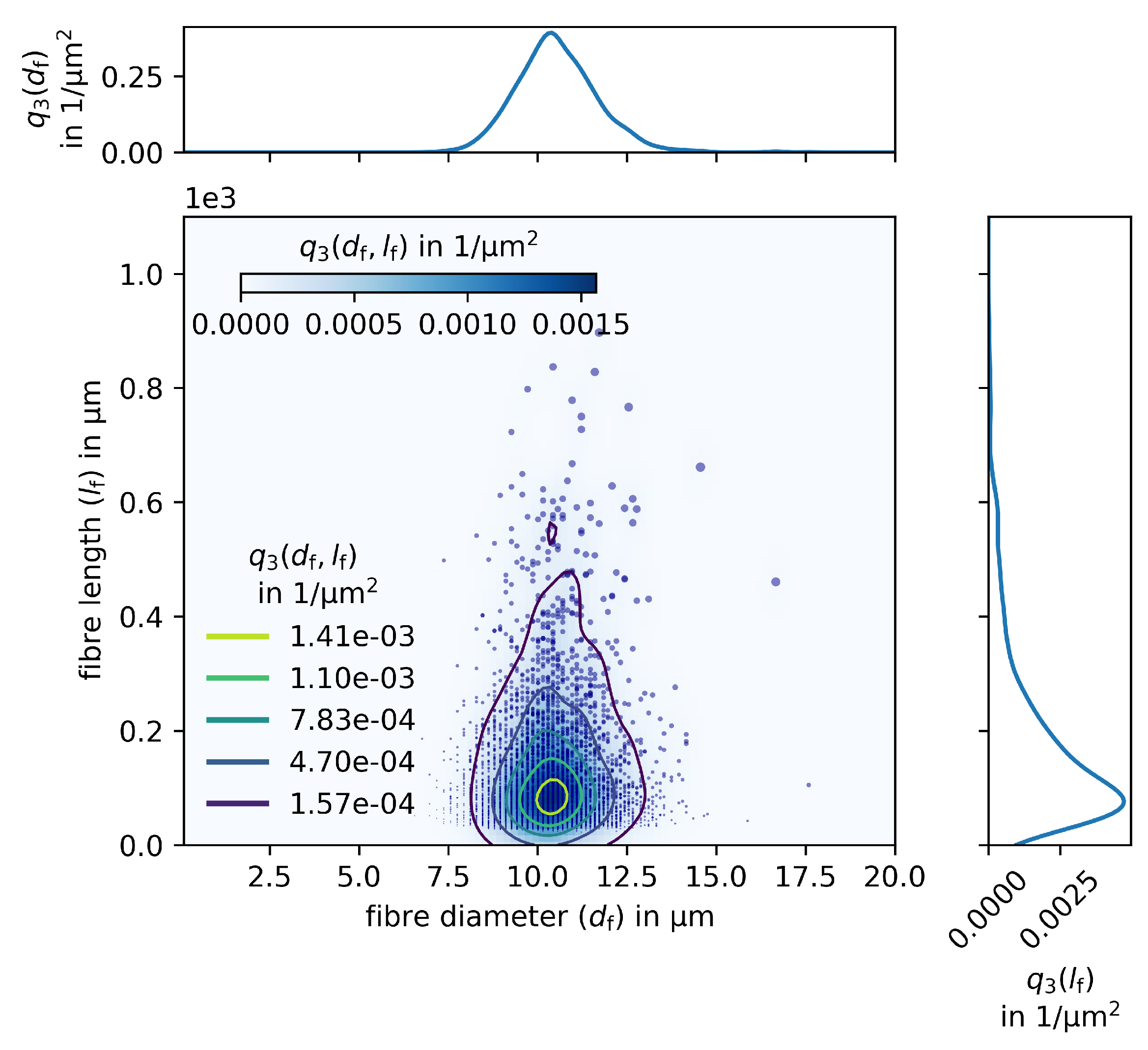
1.3. Multidimensional Characterization

In the previous sections, we established the critical need for 3D particle-discrete data and discussed the methods to create such datasets. To access the full potential of such datasets, we now have to use them for the analysis of more than one property at a time—called multidimensional analysis.

Two methodologies should be discussed here: the kernel density estimation (KDE) and the copula approach. KDE, as part of descriptive statistics, acts as a sophisticated alternative to histograms, smoothing the distribution of data points using a bandwidth parameter to create a continuous, non-parametric joint probability distribution. The KDE is a visual estimation of how two properties such as particle size and shape co-occur [17,18,19,20]. This helps visualize how these properties are distributed across the sample set, highlighting regions where certain sizes tend to correlate with certain shapes, for example. Figure 3 shows four different particle datasets downloaded from the PARROT particle database [21], further discussed in Section 5.1.

The image presents kernel density estimates for the two-dimensional number-based distribution of the longest particle dimension (principal axis 1, or rather the Feret max of the bounding box) vs. the particles’ sphericity of these four particle systems: mica (Figure 3a), soda-lime glass (Figure 3b), limestone (Figure 3c), and quartz (Figure 3d). All particle systems were produced through a crushing process, except for soda-lime glass, which was created via a spraying process. Density increases from white to dark blue. Marginal distributions along the top and right axes provide a 1D projection of the data. An SEM image displays representative particles from each sample. The additional contour lines indicate the same regions and are good for comparative purposes, which can be seen in Figure 4.

Here, limestone is plotted as a comparison to ${\mathrm{Al}}_2$, shown as number-based (Figure 4a) and particle volume-weighted (Figure 4c). Here, only a look at the sphericity shows a clear separation of the two 2D distributions. The same visualization is performed for comparing limestone with mica (Figure 4b,d). Looking at the SEM images in Figure 3, it is obvious that both marginals must show significant differences. But comparing the areas covered shows an example of how strong the difference between number-based and volume-weighted distribution can be.

The copula approach [22,23] models dependencies by first considering the marginal distribution functions of the parameters and then applying a copula function to capture their relationships [24,25]. Unlike KDE, which directly analyzes data points as a descriptive method, the copula method focuses on the joint behavior of marginal distributions. By separating individual distributions, such as size and shape, from their dependency structure, copulas provide a flexible framework for modeling complex interactions.

One possible workflow could be starting with the KDE approach as it can be performed intuitively without a deeper analysis of the characteristics of the marginal distributions. A subsequent copula-based analysis can then provide further insights into the interactions. Furthermore, the copula can be very helpful if there are more than two dimensions to consider. Consequently, there is a need for an increased sample size in terms of particle number, which is known as the curse of dimensionality [26]; this effect does not exist for the copula modeling. The copula-based method is used, e.g., in the multi-scale particle analysis [27] summarized in Section 4.1.

At this point, it should be noted that the multidimensional representation and analysis of particle-discrete data is not limited to the inherent properties of a particle system, but can be extended, for example, to the description of separation processes, which is one of the main motivations of the SPP 2045 priority program mentioned at the beginning.

2. X-Ray Tomography as a Key Technique for 3D Particle-Discrete Analysis

X-ray tomography has become a standard tool in material science [28,29], biology [30], hydrology [31], geoscience [32], and industry [33,34] over the past three decades. Early work in particle technology [35,36] evolved from 2D sectional imaging of minerals [37], while X-ray tomography was already established in medicine. Though synchrotron-based methods offer high resolution and fast measurements, they remain less accessible. Meanwhile, laboratory-based devices have advanced significantly, catching up in resolution and progressing from micro- [38] down to medium nano-scale [39].

In the following, we will focus on a micro-CT system (ZEISS, Xradia 510 VERSA, Oberkochen, Germany) equipped with an additional microscope optic to achieve high voxel resolution down to $0.3$ $\mu$$\mathrm{m}$, often called X-ray microscope (XRM). All technical details regarding the measurement parameters can be found in the referenced publications within the specific sections. They should only serve to provide better understanding of the following sections, which describe the main factors influencing a quantitative particle analysis as the foundation of a particle-discrete description. We will limit ourselves to the main influencing factors from the perspective of the particle system. In the standard workflow, these are the sample properties, the measurement parameters, the properties of the raw image data, and the properties of the pre-processed image data. In brief, these points should motivate the subsequent section on adapted sample preparation and clarify the question of what can be done to optimize the sample in order to minimize the influence of the mentioned factors.

2.1. X-Ray Microscopy

Due to its non-destructive nature, X-ray tomography became more and more interesting for determining the geometric properties and internal structure of single particles. Figure 5 shows an exemplary workflow to capture a 3D particle sample.

A typical lab-based system features a polychromatic X-ray source, where electrons from a cathode accelerate toward a target anode (e.g., tungsten), generating X-ray photons. The interaction volume is bulb-shaped, producing two sorts of radiation: characteristic X-rays, whose energy depends on the target material and is useful for chemical analysis (though irrelevant here), and bremsstrahlung, a continuous spectrum shaped by filtering (low-energy limit) and electron acceleration voltage (high-energy limit). The chosen filter and voltage define the usable spectrum. Ensuring temporal and spatial stability of this interaction is crucial for minimizing image unsharpness on the detector.

After passing through the X-ray tube aperture and sample, the conical beam is projected onto a 2D flat-panel detector. Unlike medical CT, where the detector moves, here the sample rotates on a stage, capturing projection images at each step. These images undergo reconstruction using algebraic, iterative, or filtered back-projection (FBP) [40], forming a 3D tomogram. Since the detector has a finite pixel size, the minimum pixel edge length is determined by the projection width divided by the number of pixels. To optimize the signal-to-noise ratio (SNR) and reduce measurement time, pixels can be combined (binning). In our setup, a 2048 × 2048 detector is binned to 1024 × 1024, linking the field of view (FOV) to voxel resolution by a factor of 1000. The impact on sample geometry is discussed in Section 3.2.

2.2. Main Factors Influencing Quantitative Particle Analysis

The overall goal of the tomographic measurement workflow is a sharp, highly resolved reconstructed dataset that is suitable not only for illustrative purposes in 3D visualization but for quantitative analysis, e.g., the determination of a distributed characteristic of the analyzed particle system. In general, it should be noted that materials with similar X-ray attenuation produce the same gray values, which cannot be assigned to a specific material phase without additional correlative methods. This problem is inherent in the measurement method and will not be discussed further here. The interested reader is referred to a basic introduction to the subject of X-ray imaging [40]. Within the following section, we will discuss the main influencing parameters coming from sample preparation, measurement, and image processing.

2.2.1. Particle Sample

To ideally prepare particle samples for image data evaluation, several criteria need to be met. This involves adapting established methods from 2D analysis techniques such as those used in SEM [41] and transmission electron microscopy (TEM) [42] to the requirements of 3D tomographic characterization [36,43,44]. To stabilize the particles to be scanned for several hours, necessary for a sufficiently long exposure time to obtain a series of projection images, epoxy resin can be used. In liquid state, the particles can be dispersed well and mixed with the resin. After hardening, the matrix is stable and the particles cannot move. The critical point is the significantly long curing time in the range of hours which enables particle segregation as a function of particle size and density, as can be seen in Figure 6a,b.

Furthermore, there is nothing to keep the particles at a distance since the particles have a tendency to agglomerate in the organic liquid. In the reconstructed images, there are always spots where the particles physically touch each other. Figure 6c shows an exemplary cut section. If the volumetric concentration of the particles within the epoxy is low, segregation also leads to a very large volume with a significantly different behavior. Here, only a very limited number, as shown in Figure 6d, or even no particles are visible. The described effect is shown in Figure 6e. Removing these regions before scanning would require a detailed pre-analysis, which would be impractical. The exclusion of small and/or less dense particles is critical because it alters the particle system and thus intentionally manipulates the measurement result. Significantly different sectional images are also not advantageous for automated processing with regard to subsequent image post-processing to generate the discrete-particle data. How particles can nevertheless be immobilized without coming into contact with each other we will show in Section 3.

2.2.2. Measurement Setup

With the analytical view from the perspective of the particle system, only the structural resolution counts for the actual measurement. A high voxel resolution can be achieved very easily by increasing the geometric magnification when increasing the source–detector distance or increasing the optical magnification by selecting a another objective lens in the case of XRM. Whether this increased voxel resolution helps to actually generate more valuable information on the projection image is the crucial question. In optics, this is referred to as “empty magnification”. The magnification is then no longer converted into a recognizable resolution of object details. Consequently, voxel resolution represents an idealized, theoretical number achievable under perfect conditions, disregarding several critical factors: (1) artifacts stemming from the measurement method, (2) sample-related artifacts, (3) system configuration, which directly impacts the measurement (see Figure 7), and (4) limitations in reconstruction and image post-processing. Each of these factors can significantly affect image quality. Therefore, the primary goal is to understand and mitigate these effects to optimize the actual structural resolution.

2.2.3. Artifacts

When talking about imaging techniques, artifacts are unwanted visible features that do not show the true details of the original object, like the 3D object we want to picture. Understanding artifacts is crucial, as it enables the identification and correction of image processing errors, which is especially important when working with high-resolution images. In the next section, only artifacts will be discussed that are relevant for 3D particle-discrete analysis. More details can be found in [45,46,47].

Highly X-ray-absorbing material phases change the polychromatic spectrum of the X-ray source to the extent that hardly any low-energy photons reach the scintillator. In the subsequent reconstruction, the regions of these phases appear to glow in comparison to their surroundings, and streak-like structures often appear, as exemplified in Figure 6f. This effect, called beam hardening (BH), can also occur at sharp edges and spikes. It is important to recognize that evaluating BH solely through projection images results in underestimating their effect on the final reconstructed image data.

If the embedding matrix is not completely stable, the embedded particles may shift during measurement. Furthermore, if the object’s position changes in addition to its rotational movement between individual projection images, the reconstruction algorithm may produce shadow images with varying degrees of offset. These obvious artifacts are evidence of strong object movements in the range of several percent of the object dimensions and are easy to recognize and correct during a new measurement; see Figure 6g. Smaller movements in the voxel size range are more critical. These create a blur that is difficult to identify without a reference measurement.

The preceding discussion leads to an artifact that is due to the nature of the image data. No matter how the signal is recorded, in the end it is transformed into rows and columns of a pixel image. A discrete pixel in the reconstructed sectional image has a certain gray value, and adjacent pixels have the same or a different one. Information is only generated when the gray value changes, e.g., at interesting structures such as for the particles compared to the matrix (when the particle and matrix have different attenuating properties) or within the particles at cracks, pores, phase changes, or inclusions. As the gray value change is not infinitely steep, but gradual, there are voxels in the volume that are affected by this gradient. Basically, this is a kind of averaging of different attenuation properties occurring in all neighboring voxel volumes, which is why it is also called the partial volume effect (PVE) [48]. Coming back to particle-discrete data, the image on the left in Figure 7 shows two physically touching particles that were not perfectly segmented after image post-processing. The gap between the particles was not large enough to create voxels with a gray value significantly different to the particle gray value, so it was assigned to the particle. The key issue is that two adjacent particles with a gap that is too small are likely to be mistaken for a single particle during automatic evaluation. The subsequent rejection of such artificial agglomerates needs additional image processing steps. On the other hand, the misinterpretation of particle voxels assigned to the background phase could lead to an artificial cut through the particle, which is called over-segmentation (see Figure 7—right). This should be critically examined, as it increases the number of particles in the virtual sample and skews the distribution toward smaller particles. This is the opposite of under-segmentation, which artificially raises the proportion of larger particles within the particle size distribution.

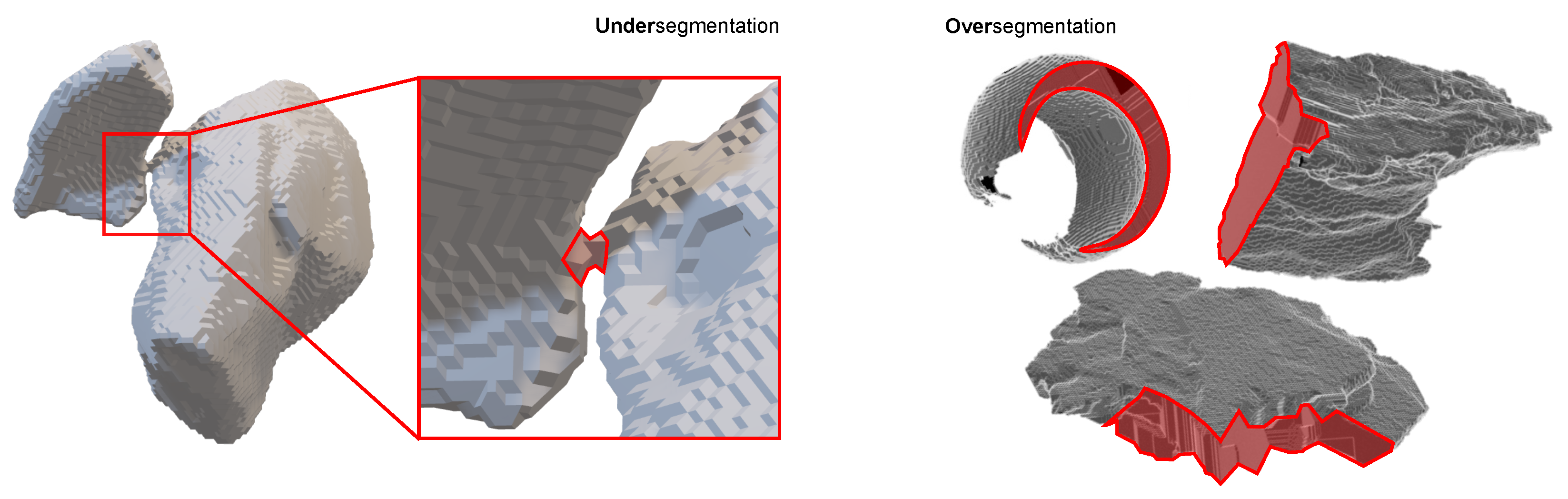
2.2.4. Image Processing

Image processing can be divided into two main steps, image pre-processing, before or during the tomographic reconstruction process, and post-processing, after the reconstruction. Important pre-processing steps are beam hardening correction; normalization to standardize brightness and contrast across different series of projection images; correction of misalignment and motion, not only of the sample but also for source and detector; and noise filtering. These steps are crucial for optimum image quality but should not be of further concern here. The interested reader is referred to [40].

Image post-processing is usually performed on the reconstructed image stack and includes methods like noise reduction, contrast enhancement, further artifact correction, and edge sharpening. Considering the main objective, namely a quantitative analysis of the discrete particle data, the most important step is the separation of the particles, which are only recognized as individual sub-volumes by automatic evaluation algorithms after correct virtual separation. This process is called segmentation.

As discussed previously, only one “binding” voxel is enough to create under-segmented particle assemblies. Conversely, over-segmentation can happen and a single particle is incorrectly divided into multiple entities during image processing. The right-hand side of Figure 7 shows examples where parts of the particles are virtually cut off.

Figure 8a shows a reconstructed gray value image representing one section in a specific height of the tomogram of the particle sample.

In this example, we used the freeware tool Ilastik [49] (version 1.4.0,post1) to perform the image segmentation. Here, a standard workflow is to first create a classifier based on pixel information only. Here, the material phase is distinguished from the background phase. The result is a map of probabilities that are loaded with the original image data in a second step. Now it is possible to perform an automated routine running through the whole image stack identifying individual volumes of the material phase that will be color-coded; see Figure 8b. This color code is later translated into a unique gray value, called a label, that finally can be used by another automated routine to acquire quantitative data.

The disadvantage of this method is that the internal gray value distribution of each particle is lost after labeling. However, the information of an aggregated gray value or even a histogram for each individual particle is essential for the particle-discrete analysis of the distribution of the material phases. Since the gray value is an intrinsic feature of the voxel dataset, it can easily be extracted as particle-discrete data and compared with other 3D image data with the same measurement parameters after appropriate scaling. Figure 8b,d shows the extracted particle with the corresponding gray value histogram generated with the freeware tool ImageJ [4]. An example of conventional sectioning is shown in Figure 8e. Scanning the images from the top left to the bottom right reveals how difficult and error-prone this process of obtaining particle information would be if only one of these sectional images were available.

2.2.5. Summary

Assessing the accuracy of quantitative image data is difficult without a comprehensive understanding of the particle sample, the measurement system, the raw data generated with this system, and the image processing. In contrast to image processing, however, the effects during image generation cannot be separated from each other as a kind of layer; they merge into a more or less good result in the reconstructed image. In this sense, “good” is the state of highest possible practical structural resolution and sharpness, and lowest noise. Figure 9 summarizes the influencing factors.

How the preparation of the particle sample positively support this process will be discussed in the next section.

3. Supporting Particle Sample Preparation Techniques

3.1. General Aspects

The 3D sample preparation method presented here enables the creation of a homogeneous and representative particle sample of a statistically relevant quantity, eliminating the stereological bias. Both presented methods, wax-based and epoxy-based, ensure two key requirements: first of all, the rotational symmetry of the sample to guarantee uniform X-ray penetration lengths, and secondly, a sample size that fits to the desired FOV. The latter is crucial to prevent region of interest (ROI) tomography [50], also called truncated tomography [51], within the sample, which leads to increased exposure times due to sample thickness and a greater number of required projections. The adapted sample preparation also reduces the likelihood of artifacts caused by material outside the FOV. Although appropriate segmentation algorithms are available, e.g., in ImageJ [4] or Ilastik [49], going one step back to the sample and finding a preparation method that creates enough space between single particles seems to be a more reasonable approach.

3.2. Particle Sample Requirements

Challenges in tomography include sample geometry, grade of dispersion, homogeneity, and the statistical representativeness of the particle sample. The following short section starts with an overview of the mentioned points before introducing both methods in detail, which are applied for the studies presented in Section 4. A detailed description is given in [47].

3.2.1. Geometry

The geometry of the sample has a direct influence on the image quality and the achievable structural resolution of the measurement. As discussed in Section 2.1, voxel resolution and FOV are firmly linked. In other words, it is not possible to scan large samples with the highest possible resolution. Although the tomography of very small ROI is possible, it requires a significant increase in the acceleration voltage and power of the X-ray source. Highly accelerated electrons produce highly energetic X-ray photons that are able to penetrate larger volumes and make ROI tomography possible. Note that these electrons also generate a significantly larger interaction bulb in the target material, which, in addition to the thermal fluctuations of this region, has a negative influence on the expansion of the X-ray point source, i.e., the starting point of the cone beam, resulting in (penumbral) blurring. Furthermore, material contrast is lost, as there are more and more high-energy X-ray photons in the spectrum, which easily penetrate the larger sample diameter, but are hardly absorbed by light phases. Both effects show that optimum results can only be achieved when the sample geometry is adapted to the size of the structures that are to be resolved.

3.2.2. Dispersity and Homogeneity

The optimal case would be additional space between a particle and all its neighbors to guarantee the separation volume being much larger than the PVE blurred voxels, which cannot be eliminated. Besides the dispersion, all particles should be homogeneously distributed within the sample volume no matter their particle size or density. Both requirements are quite challenging and have not been adequately met in the past, e.g., the adhesion of individual particles to an adhesive tape that is rolled up for measurement [52] or the embedding of particles in a rotating gravitational field during solidification [1]. Both methods are not suitable for accommodating a statistically relevant quantity of representative particles in a very small volume.

3.2.3. Statistics

When dealing with distributed properties, it is essential for the particle sample to be representative of the entire population. Sampling particulate materials involves a series of steps: extracting sub-samples (like from a mineral deposit), creating a homogeneous mixture, conditioning the sample, and finally, sample splitting to obtain a representative sample. Each of these steps can introduce errors [53]. Even when measuring the entire sample in cases of very small quantities, it is essential to ensure that there are enough particles within the FOV to achieve a statistically reliable analysis. All measurement volumes, regardless of their size, must be representative of the whole sample. One major advantage of 3D analysis in this regard is that the number of particles increases rapidly compared to 2D analysis methods where the statistical challenge is addressed by measuring a large number of polished cut sections, mapping a large area, or generating a continuous stream of particles passing the detector, like in DIA [16]. An additional point is the particle size distribution itself. If this distribution is very narrow and follows a known type, e.g., normal, then it is significantly different to a distribution that is very wide with a non-negligible share of large particles, or maybe with a multi-modal shape. It has to be guaranteed that each individual particle has the same chance to enter the FOV [54].

3.2.4. Validation

When setting up a workflow for 3D tomographic acquisition, it is always good to have an idea about the expected result, even if the available image data are only 2D. Comparing the quantitative results of image-based measurement techniques with results from other image-based methods is ideal. Cross-validating quantitative results from tomographic measurements with 2D image analysis methods like optical microscopy or SEM has been very effective, as can be seen in [27,43], respectively. “Optical inspection” is crucial for identifying unique features in the particle sample, such as satellite particles or hollow structures, which could further complicate image processing. This is performed not for calibrating the system (due to stereological bias) in the workflow of tomographic image data evaluation, but for highlighting potential errors.

3.3. Shock Freezing of a Highly Viscous Matrix

We were looking for a sample preparation method that is particularly suitable for brittle particles as it avoids the need for mechanical dispersion steps other than stirring. The method involves a histological wax with a melting point between 59 ° C and 61 ° C as the embedding matrix. The process includes dispersing the particles in wax and then sampling the suspension using a pre-heated plastic tube to prevent uncontrolled solidification and radial segregation of the wax before sampling is completed. After controlled suction with a self-constructed automated extraction unit [25], the sample is instantly solidified by applying a freezing spray.

The method is beneficial as it minimizes the risk of damaging brittle particles during preparation, making it ideal for sensitive samples in XRM analysis. The wax method was first tested and evaluated with a one-component idealized spherical glass particle system [43] and later used for a study with a mixture of fibers and spheres over multiple length scales [27], later discussed in Section 4.1. With the wax method, we were able to create a sample of a homogeneously dispersed particle mixture without applying mechanical stress that destroys the glass fibers and alters the particle property distributions.

3.4. Epoxy Embedding Adding Low-X-Ray-Attenuating Spacer Particles

The epoxy-based sample preparation method effectively suppresses segregation by using carbon black nanoparticles as the spacer [44]. The method is designed to minimize the negative influence of particle sedimentation during the curing process of the epoxy resin. The carbon black nanoparticles, being nearly X-ray-transparent and significantly smaller than the voxel resolution, serve to maintain spatial separation between the particles of interest. Previously implemented for 2D mineralogical analysis [9,11,17], the method has now been adapted and validated for 3D tomographic experiments. While our discussion focuses on its application in X-ray tomographic analysis, the method is also suitable for laser milling [55] and serial sectioning [6].

However, for a correlative analysis with an additional higher resolution imaging modality, discussed in Section 4.2, highly absorbing mineralogical samples of the same size would have led to significant artifacts and increased exposure times, needing a reduction in sample size. This allowed the use of a laser mill to create a cylinder with a diameter of 60 $\mu$$\mathrm{m}$ from manually cut bars, suitable for both FIB-SEM analysis and for accommodating the constraints of highly absorbing phases.

4. Application

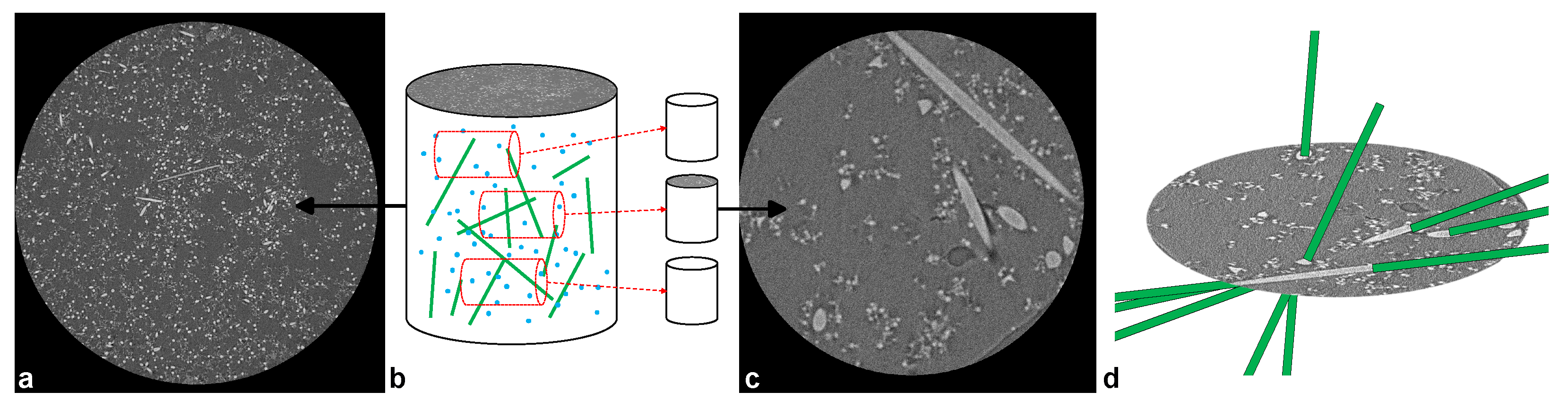
4.1. Multi-Scale Analysis

Multi-scale analysis focuses on imaging the same sample at different spatial resolutions and FOVs. The analysis often starts with a large area scan at lower resolution to identify the ROI, followed by high-resolution scans of selected areas. This is useful to bridge the gap between macro-structural and micro-structural features, e.g., to link bulk material properties with fine structural details.

Tomographic datasets can have a multi-scale structure of two types. The first type refers to a particle system with a characteristic particle geometry within the same order of magnitude, but the particles possess recurring, finely structured surface features. The latter need to be analyzed with a higher resolution which is possible only for selected ROIs. The second case is a mixture of disperse particle systems, at least one of which differs from the other by an order of magnitude in size. We analyzed this case using the wax-based sample preparation method [27].

This study investigates a combination of fibers that are several hundred micrometers long and spherical particles smaller than 10 $\mu$$\mathrm{m}$ in diameter. Figure 10 shows an example of the particle system of the fibers by plotting the very narrowly distributed fiber diameter against the very widely distributed fiber length. It should be noted that the slight asymmetry of the variation in the specified fiber diameter from 10 $\mu$$\mathrm{m}$ to larger values can be explained by the previously mentioned PVE.

When adjusting the FOV to encompass the length of the fibers, the voxel size is decreased to a point where only a partial representation of the spherical particles is possible, as they fall well below the voxel size; see Figure 11a. Therefore, sub-samples are taken at different heights of the initial sample to have a statistically significant amount of particles; see Figure 11b,c. This was performed by manually cutting the sample cylinders into small bars of about 300 $\mu$$\mathrm{m}$ diameter, matching the XRM’s minimum voxel size of 400 $\mathrm{n}$$\mathrm{m}$. The scans of these bar scans then serve as an overview to select sub-volumes for high-resolution nano-CT scans, applicable to both spherical and fiber particles in multi-scale analysis, with a voxel size of 64 $\mathrm{n}$$\mathrm{m}$. Conversely, scanning the spherical particles at high resolution does not capture the full length of the fibers. Figure 11d shows that in most cases only oval-shaped structures appear in the cut section. The comprehensive characterization of the entire system is achieved only by integrating two steps of magnification.

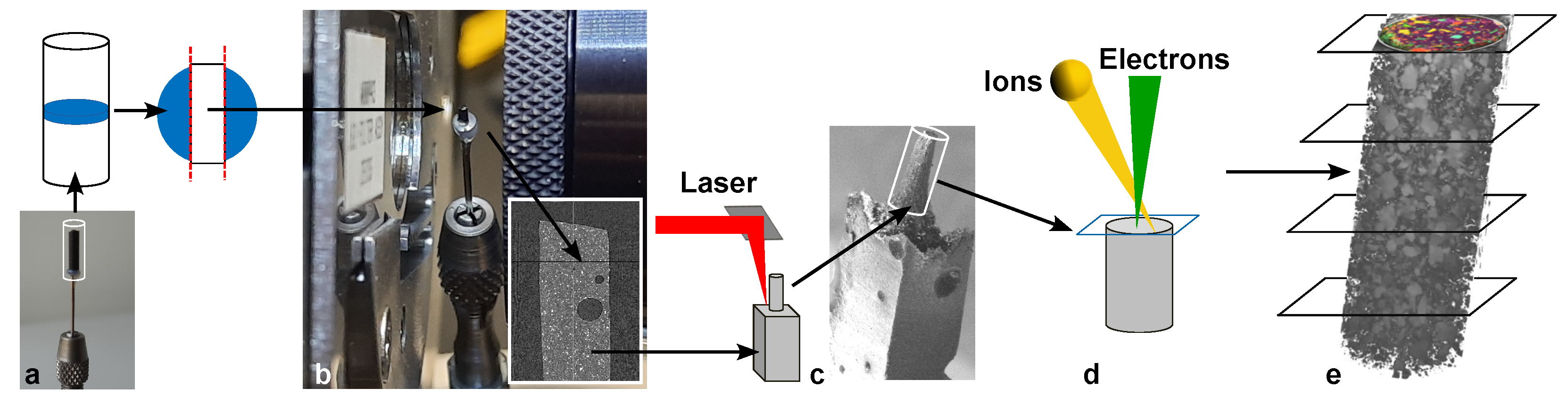
4.2. Correlative Analysis

Correlative analysis combines X-ray tomography with other imaging methods (e.g., electron microscopy, optical microscopy, or spectroscopy) to provide complementary information. Here, the aim is to correlate different datasets, e.g., combining XRM for 3D structure with SEM for surface details or EDS for elemental composition. This enables a more comprehensive analysis by integrating different contrasts, resolutions, and information types. So, it is not only about enhancing and validating the primary measurement results but also uncovering additional information that could not be accessed by a single method [56]. This approach is particularly valuable for comprehensive material characterization, as it allows the strengths of different imaging techniques to be combined to provide a more complete picture of the sample.

It has to be emphasized here that the sample preparation strategy plays a critical role in optimizing the analysis process. For instance, reducing the sample volume between steps, as demonstrated in some studies, can significantly decrease the time needed for acquisition. This is particularly advantageous in applications like nano-tomography, where the feasibility of the measurement already depends on such optimizations.

Figure 12 shows how we implemented a workflow utilizing multiple measurement devices to unravel the 3D composition of multi-phase particles [57]. We used epoxy preparation to produce samples that only lose their structural integrity in locations when exposed to high-energy radiation (laser, ions) and thus enable more or less flat cut surfaces without a subsequent change of the structure.

5. Challenges and Future Directions

5.1. The FAIR Principle Applied to Particle Data

In accordance with the FAIR principle [58], which is designed to ensure that scientific data are structured and stored in a manner that facilitates their findability, accessibility, interoperability, and reusability, we initiated a feasibility study to generate a particle database called PARROT [21]. The database employs a straightforward web interface, allowing users to filter particle-discrete data based on a range of parameters before downloading datasets in different levels of aggregation. The highest level contains the reconstructed tomographic data as a stack of tagged image file format (TIFF) images, accompanied by a segmented image stack. Both datasets are securely stored within an existing repository, OpARA [59], ensuring long-term availability via digital object identifier (DOI) references. Figure 13 shows exemplary particles from all six particle systems downloaded from the database.

A key feature of the PARROT database is its comprehensive metadata framework, which plays a crucial role in describing the context of each dataset. Metadata includes details about the sample preparation method, measurement conditions, and image processing parameters, ensuring that users can accurately interpret the data and integrate them into their research. Automated metadata extraction is implemented to improve dataset consistency and minimize manual errors.

Beyond data storage, the database architecture follows a relational database model, which efficiently organizes particle-discrete data and metadata while reducing redundancy. This enables fast queries for dataset retrieval, making the system scalable for future expansions. The integration with OpARA further enhances data accessibility, allowing researchers to cross-reference datasets using DOIs in scientific publications.

To demonstrate the value of PARROT, three practical use cases are presented in [21], showcasing its applications in 3D particle analysis, statistical and multivariate parametric modeling, and numerical process simulations. The latter leverages lattice Boltzmann methods to simulate fluid–particle interactions, providing critical insights into filtration and transport processes.

5.2. 3D Multi-Phase Particle-Discrete Datasets

As described in the previous paragraph, correlative imaging enables the acquisition of 3D particle-discrete phase information. Each voxel of a 3D particle has a specific gray value. If these are clearly separated from each other and there are no mixed phases, as in Figure 14a–c, it is possible to separate the phases, i.e., to segment them with phase accuracy.

However, if there are intergrowth and mixed phases, visualization becomes challenging. Figure 14d shows one possibility. Each individual volume of voxels, i.e., each particle, is saved as a histogram. If the density of the histogram is color-coded again in gray values, the maximum in white, the minimum in black, and the values are plotted horizontally, a line with distributed gray values is obtained. In simple terms, this is the view of the histogram from above. A random selection from the entire dataset, in this example 1000 particles, is arranged according to the width of the distribution from narrow to wide and all histogram lines are stacked on top of each other. This results in some kind of fingerprint for each particle system and thus comparisons can be made easily. Of course, this is just one example, but it shows that there is a large field of application for new visualization methods, some of which still need to be established, in order to visualize the data in a meaningful way.

Although the theoretical principles of the 3D characterization of particles have been discussed in detail in the past and the advantages of this method over 2D imaging and the description with equivalent sizes are obvious, it is still too rarely used in the particle characterization community. This needs to change. The relationships of particle properties are rarely one-dimensional, and when they are, they often lack precision. Particle-discrete multidimensional analysis offers a powerful tool to gain new insights on process and parameter correlations.

References

1. Erdoğan, S.T.; Garboczi, E.T.; Fowler, D.W. Shape and size of microfine aggregates: X-ray microcomputed tomography vs. laser diffraction. Powder Technol. 2007, 177, 53–63. [Google Scholar] [CrossRef]
2. Demeler, B.; Nguyen, T.L.; Gorbet, G.E.; Schirf, V.; Brookes, E.H.; Mulvaney, P.; El-Ballouli, A.O.; Pan, J.; Bakr, O.M.; Demeler, A.K.; et al. Characterization of Size, Anisotropy, and Density Heterogeneity of Nanoparticles by Sedimentation Velocity. Anal. Chem. 2014, 86, 7688–7695. [Google Scholar] [CrossRef] [PubMed]
3. Whitby, K. The Mechanics of Fine Sieving. In Symposium on Particle Size Measurement; ASTM International: West Conshohocken, PA, USA, 1959; pp. 3–25. [Google Scholar] [CrossRef]
4. Rueden, C.T.; Schindelin, J.; Hiner, M.C.; DeZonia, B.E.; Walter, A.E.; Arena, E.T.; Eliceiri, K.W. ImageJ2: ImageJ for the next generation of scientific image data. BMC Bioinform. 2017, 18, 529. [Google Scholar] [CrossRef] [PubMed]
5. Pham, D.T.; Dimov, S.S.; Petkov, P.V.; Petkov, S.P. Laser milling. Proc. Inst. Mech. Eng. Part B J. Eng. Manuf. 2002, 216, 657–667. [Google Scholar] [CrossRef]
6. Spowart, J.E. Automated serial sectioning for 3-D analysis of microstructures. Scr. Mater. 2006, 55, 5–10. [Google Scholar] [CrossRef]
7. Burnett, T.L.; Kelley, R.; Winiarski, B.; Contreras, L.; Daly, M.; Gholinia, A.; Burke, M.G.; Withers, P.J. Large volume serial section tomography by Xe Plasma FIB dual beam microscopy. Ultramicroscopy 2016, 161, 119–129. [Google Scholar] [CrossRef]
8. Lätti, D.; Adair, B. An assessment of stereological adjustment procedures. Miner. Eng. 2001, 14, 1579–1587. [Google Scholar] [CrossRef]
9. Sutherland, D.N.; Gottlieb, P. Application of automated quantitative mineralogy in mineral processing. Miner. Eng. 1991, 4, 753–762. [Google Scholar] [CrossRef]
10. Schulz, B.; Sandmann, D.; Gilbricht, S. SEM-Based Automated Mineralogy and Its Application in Geo- and Material Sciences. Minerals 2020, 10, 1004. [Google Scholar] [CrossRef]
11. Shaffer, M. Sample preparation methods for imaging analysis. In Proceedings of the Geometallurgy and Appl. Mineralogy 2009, Conference of Mineralogists, Cape Town, South Africa, 23–27 November 2009. [Google Scholar]
12. Macho, O.; Kabát, J.; Gabrišová, L.; Peciar, P.; Juriga, M.; Fekete, R.; Galbavá, P.; Blaško, J.; Peciar, M. Dimensionless criteria as a tool for creation of a model for predicting the size of granules in high-shear granulation. Part. Sci. Technol. 2019, 38, 381–390. [Google Scholar] [CrossRef]
13. Köhler, U.; Stübinger, T.; Witt, W. Laser-Diffraction Results From Dynamic Image Analysis Data. In Proceedings of the Conference Proceedings WCPT6, Nuremberg, Germany, 26–29 April 2010. [Google Scholar]
14. Gay, S.L.; Morrison, R.D. Using Two Dimensional Sectional Distributions to Infer Three Dimensional Volumetric Distributions—Validation using Tomography. Part. Part. Syst. Charact. 2006, 23, 246–253. [Google Scholar] [CrossRef]
15. Ueda, T.; Oki, T.; Koyanaka, S. Experimental analysis of mineral liberation and stereological bias based on X-ray computed tomography and artificial binary particles. Adv. Powder Technol. 2018, 29, 462–470. [Google Scholar] [CrossRef]
16. Ulusoy, U.; Igathinathane, C. Particle size distribution modeling of milled coals by dynamic image analysis and mechanical sieving. Fuel Process. Technol. 2016, 143, 100–109. [Google Scholar] [CrossRef]
17. Schach, E.; Buchmann, M.; Tolosana-Delgado, R.; Leißner, T.; Kern, M.; van den Boogaart, G.; Rudolph, M.; Peuker, U.A. Multidimensional characterization of separation processes—Part 1: Introducing kernel methods and entropy in the context of mineral processing using SEM-based image analysis. Miner. Eng. 2019, 137, 78–86. [Google Scholar] [CrossRef]
18. Buchmann, M.; Schach, E.; Leißner, T.; Kern, M.; Mütze, T.; Rudolph, M.; Peuker, U.A.; Tolosana-Delgado, R. Multidimensional characterization of separation processes—Part 2: Comparability of separation efficiency. Miner. Eng. 2020, 150, 106284. [Google Scholar] [CrossRef]
19. Schach, E.; Buchwald, T.; Furat, O.; Tischer, F.; Kaas, A.; Kuger, L.; Masuhr, M.; Sygusch, J.; Wilhelm, T.; Ditscherlein, R.; et al. Progress in the Application of Multidimensional Particle Property Distributions: The Separation Function. KONA Powder Part. J. 2024, 42, 134–155. [Google Scholar] [CrossRef]
20. Buchwald, T.; Schach, E.; Peuker, U.A. A framework for the description of multidimensional particle separation processes. Powder Technol. 2024, 433, 119165. [Google Scholar] [CrossRef]
21. Ditscherlein, R.; Furat, O.; Löwer, E.; Mehnert, R.; Trunk, R.; Leißner, T.; Krause, M.J.; Schmidt, V.; Peuker, U.A. PARROT: A Pilot Study on the Open Access Provision of Particle-Discrete Tomographic Datasets. Microsc. Microanal. 2022, 28, 350–360. [Google Scholar] [CrossRef]
22. Nelsen, R.B. An Introduction to Copulas; Springer: Berlin/Heidelberg, Germany, 2006. [Google Scholar]
23. Durante, F.; Sempi, C. Principles of Copula Theory; Chapman and Hall/CRC: Boca Raton, FL, USA, 2015. [Google Scholar]
24. Furat, O.; Leißner, T.; Bachmann, K.; Gutzmer, J.; Peuker, U.A.; Schmidt, V. Stochastic Modeling of Multidimensional Particle Properties Using Parametric Copulas. Microsc. Microanal. 2019, 25, 720–734. [Google Scholar] [CrossRef]
25. Ditscherlein, R.; Leißner, T.; Peuker, U.A. Self-constructed automated syringe for preparation of micron-sized particulate samples in X-ray microtomography. MethodsX 2020, 7, 100757. [Google Scholar] [CrossRef]
26. Bellman, R.; Page, E.S. Adaptive Control Processes: A Guided Tour; Princeton University Press: Princeton, NJ, USA, 1961. [Google Scholar] [CrossRef]
27. Ditscherlein, R.; Furat, O.; de Langlard, M.; Martins de Souza e Silva, J.; Sygusch, J.; Rudolph, M.; Leißner, T.; Schmidt, V.; Peuker, U.A. Multiscale Tomographic Analysis for Micron-Sized Particulate Samples. Microsc. Microanal. 2020, 26, 676–688. [Google Scholar] [CrossRef] [PubMed]
28. Baruchel, J.; Buffiere, J.Y.; Maire, E.; Merle, P.; Peix, G. X-Ray Tomography in Material Science; Hermes Science Publications: Paris, France, 2000. [Google Scholar]
29. Stock, S.R. Recent advances in X-ray microtomography applied to materials. Int. Mater. Rev. 2008, 53, 129–181. [Google Scholar] [CrossRef]
30. Mizutani, R.; Suzuki, Y. X-ray microtomography in biology. Micron 2012, 43, 104–115. [Google Scholar] [CrossRef] [PubMed]
31. Wildenschild, D.; Vaz, C.M.P.; Rivers, M.L.; Rikard, D.; Christensen, B.S.B. Using X-ray computed tomography in hydrology: Systems, resolutions, and limitations. J. Hydrol. 2002, 267, 285–297. [Google Scholar] [CrossRef]
32. Ketcham, R.A.; Carlson, W.D. Acquisition, optimization and interpretation of X-ray computed tomographic imagery: Applications to the geosciences. Comput. Geosci. 2001, 27, 381–400. [Google Scholar] [CrossRef]
33. Brown, D.J.; Vickers, G.T.; Collier, A.P.; Reynolds, G.K. Measurement of the size, shape and orientation of convex bodies. Chem. Eng. Sci. 2005, 60, 289–292. [Google Scholar] [CrossRef]
34. Zschech, E.; Yun, W.; Schneider, G. High-resolution X-ray imaging—A powerful nondestructive technique for applications in semiconductor industry. Appl. Phys. A 2008, 92, 423–429. [Google Scholar] [CrossRef]
35. Lin, C.L.; Miller, J.D.; Cortes, A. Applications of X-Ray Computed Tomography in Particulate Systems. KONA Powder Part. J. 1992, 10, 88–95. [Google Scholar] [CrossRef]
36. Miller, J.D.; Lin, C.L. Three-dimensional analysis of particulates in mineral processing systems by cone beam X-ray microtomography. Miner. Metall. Process. 2004, 21, 113–124. [Google Scholar] [CrossRef]
37. Miller, J.D.; Lin, C.L. Treatment of polished section data for detailed liberation analysis. Int. J. Miner. Process. 1988, 22, 41–58. [Google Scholar] [CrossRef]
38. Withers, P.J.; Bouman, C.; Carmignato, S.; Cnudde, V.; Grimaldi, D.; Hagen, C.K.; Maire, E.; Manley, M.; du Plessis, A.; Stock, S.R. X-ray computed tomography. Nat. Rev. Methods Prim. 2021, 1, 18. [Google Scholar] [CrossRef]
39. Withers, P.J. X-ray nanotomography. Mater. Today 2007, 10, 26–34. [Google Scholar] [CrossRef]
40. Buzug, T.M. Computed Tomography from Photon Statistics to Modern Cone-Beam CT; Springer: Berlin/Heidelberg, Germany, 2008. [Google Scholar] [CrossRef]
41. Echlin, P. Handbook of Sample Preparation for Scanning Electron Microscopy and X-Ray Microanalysis; Springer: Cambridge Analytical Microscopy: Cambridge, UK, 2009. [Google Scholar]
42. Ayache, J.; Beaunier, L.; Boumendil, J.; Ehret, G.; Laub, D. Sample Preparation Handbook for Transmission Electron Microscopy: Techniques; Springer: Berlin/Heidelberg, Germany, 2010; p. 338. [Google Scholar]
43. Ditscherlein, R.; Leißner, T.; Peuker, U.A. Preparation techniques for micron-sized particulate samples in X-ray microtomography. Powder Technol. 2019, 360, 989–997. [Google Scholar] [CrossRef]
44. Ditscherlein, R.; Leißner, T.; Peuker, U.A. Preparation strategy for statistically significant micrometer-sized particle systems suitable for correlative 3D imaging workflows on the example of X-ray microtomography. Powder Technol. 2022, 395, 235–242. [Google Scholar] [CrossRef]
45. Davis, G.R.; Elliott, J.C. Artefacts in X-ray microtomography of materials. Mater. Sci. Technol. 2006, 22, 1011–1018. [Google Scholar] [CrossRef]
46. Boas, F.E.; Fleischmann, D. CT artifacts: Causes and reduction techniques. Imaging Med. 2012, 4, 229–240. [Google Scholar] [CrossRef]
47. Ditscherlein, R. A Contribution to the Multidimensional and Correlative Tomographic Characterization of Micron-Sized Particle Systems. Ph.D. Thesis, TU-Bergakademie Freiberg, Freiberg, Germany, 2022. [Google Scholar]
48. Soret, M.; Bacharach, S.L.; Buvat, I. Partial-Volume Effect in PET Tumor Imaging. J. Nucl. Med. 2007, 48, 932–945. [Google Scholar] [CrossRef]
49. Berg, S.; Kutra, D.; Kroeger, T.; Straehle, C.N.; Kausler, B.X.; Haubold, C.; Schiegg, M.; Ales, J.; Beier, T.; Rudy, M.; et al. ilastik: Interactive machine learning for (bio)image analysis. Nat. Methods 2019, 16, 1226–1232. [Google Scholar] [CrossRef]
50. Kyrieleis, A.; Titarenko, V.; Ibison, M.; Connolley, T.; Withers, P.J. Region-of-interest tomography using filtered backprojection: Assessing the practical limits. J. Microsc. 2010, 241, 69–82. [Google Scholar] [CrossRef]
51. Katsumata, A.; Hirukawa, A.; Okumura, S.; Naitoh, M.; Fujishita, M.; Ariji, E.; Langlais, R.P. Effects of image artifacts on gray-value density in limited-volume cone-beam computerized tomography. Oral Surg. Oral Med. Oral Pathol. Oral Radiol. Endodontol. 2007, 104, 829–836. [Google Scholar] [CrossRef]
52. Tsuchiyama, A.; Sakurama, T.; Nakano, T.; Uesugi, K.; Ohtake, M.; Matsushima, T.; Terakado, K.; Galimov, E.M. Three-dimensional shape distribution of lunar regolith particles collected by the Apollo and Luna programs. Earth Planets Space 2022, 74, 172. [Google Scholar] [CrossRef]
53. Gy, P.M. The sampling of particulate materials—A general theory. Int. J. Miner. Process. 1976, 3, 289–312. [Google Scholar] [CrossRef]
54. Hutschenreiter, W. Fehlerrechnung und Optimierung bei der Probenahme. Freib. Forschungshefte 1975, A 531, 8. [Google Scholar]
55. Leone, C.; Papa, I.; Tagliaferri, F.; Lopresto, V. Investigation of CFRP laser milling using a 30W Q-switched Yb:YAG fiber laser: Effect of process parameters on removal mechanisms and HAZ formation. Compos. Part A Appl. Sci. Manuf. 2013, 55, 129–142. [Google Scholar] [CrossRef]
56. Furat, O.; Leißner, T.; Ditscherlein, R.; Šedivý, O.; Weber, M.; Bachmann, K.; Gutzmer, J.; Peuker, U.A.; Schmidt, V. Description of Ore Particles from X-Ray Microtomography (XMT) Images, Supported by Scanning Electron Microscope (SEM)-Based Image Analysis. Microsc. Microanal. 2018, 24, 461–470. [Google Scholar] [CrossRef]
57. Englisch, S.; Ditscherlein, R.; Kirstein, T.; Hansen, L.; Furat, O.; Drobek, D.; Leißner, T.; Apeleo Zubiri, B.; Weber, A.P.; Schmidt, V.; et al. 3D analysis of equally X-ray attenuating mineralogical phases utilizing a correlative tomographic workflow across multiple length scales. Powder Technol. 2023, 419, 118343. [Google Scholar] [CrossRef]
58. Wilkinson, M.D.; Dumontier, M.; Aalbersberg, I.J.; Appleton, G.; Axton, M.; Baak, A.; Blomberg, N.; Boiten, J.W.; da Silva Santos, L.B.; Bourne, P.E.; et al. The FAIR Guiding Principles for scientific data management and stewardship. Sci. Data 2016, 3, 160018. [Google Scholar] [CrossRef]
59. OpARA. Open Access Repository and Archive. Available online: https://opara.zih.tu-dresden.de/xmlui/ (accessed on 12 February 2025).
Figure 1. Exemplary particle systems as 2D projection with their representative in Fourier space. Mono-disperse spherical particles: (a) large, (b) small, and (c) fibers. (d) shows the measurement setup of the laser diffraction system creating a diffraction pattern of an ejected particle system projected on a semi-circled flat panel detector.
Powders 04 00012 g001
Figure 2. An (a) exemplary particle, selected based on the longest dimension of its virtual cut section, extracted from an X-ray tomographic 3D volume. Random rotations produce significantly different values due to variations in the number of cut sections. The particle with the minimum and maximum number of cut sections is highlighted in blue and red, respectively. (b) Examples of sectional surfaces from a 2D preparation, illustrating different grinding depths along the z-axis. (c) An example of a sectional plane at different rotations, as analyzed using SEM-based automated mineralogy.
Powders 04 00012 g002
Figure 3. Multidimensional visualization using kernel density estimates for four different particle systems: (a) mica, (b) soda-lime glass, (c) limestone, and (d) quartz. Density is represented by color, ranging from white (low density) to dark blue (high density), with contour lines following the same color scheme. The top and right sides display the corresponding marginal distributions. The SEM image presents representative particles from each sample.
Powders 04 00012 g003
Figure 4. Multidimensional visualization of kernel density estimates: (a,c) limestone (red) vs. Al 2 O 3 (blue) and (b,d) limestone vs. mica, shown as (a,b) number-based and (c,d) volume-weighted.
Powders 04 00012 g004
Figure 5. Exemplary workflow of a tomographic particle measurement. The X-rays are penetrating the embedded particle sample non-destructively and are projected on a scintillator screen in a first magnification step, where they are converted to visual light. A macroscopic optic magnifies the image a second time and projects it onto a detector. Multiple of these images, recorded under different sample rotating angles, result in a set of projection images that is converted to a 3D image stack via tomographic reconstruction, which enables particle-discrete datasets to be extracted by extensive image processing that can be used further for quantitative analysis. Note that for illustrative purposes a comparatively large particle system is used. The presented studies deal with particles around one order of magnitude lower.
Powders 04 00012 g005
Figure 6. Epoxy-embedded particle sample (a) showing segregation along the sample height; (b) representative 3D volume virtually cut in different heights (c) with cut sections containing large touching particles that are (d) separated, but with very few particles, and (e) very small particles occurring sporadically in the region of the sample volume. (f) Highly X-ray-absorbing particles generating beam-hardening artifacts and (g) motion artifacts, and (h) and an exemplary mica particle from the example captured by SEM.
Powders 04 00012 g006
Figure 7. Under-segmented particles only connected by a single voxel (left) and three examples of particles showing typical patterns (outlined) as sign of over-segmentation (right).
Powders 04 00012 g007
Figure 8. (a) Results from a raw tiff (b) segmented with the software package Ilastik [49] resulting in a labeled particle-discrete dataset. (c) An exemplary particle from this dataset (d) with the corresponding histogram and (e) exemplary cut sections from the same particle showing the significantly different gray values depending on the cut height.
Powders 04 00012 g008
Figure 9. Overview of elements affecting quantitative image data analysis. This includes the system setup, which directly impacts the measurement. Both the measurement and the particle sample can introduce artifacts, influencing the projection image quality. Additionally, the reconstruction process can modify the final tomogram’s image quality, relevant for quantitative analysis, summarizing image reproduced from [47].
Powders 04 00012 g009
Figure 10. Visualization of the fiber particle system, showing the narrowly distributed fiber diameter against the widely distributed fiber length. The slight asymmetry in fiber diameter variation from 10 n m to larger values is due to the previously mentioned PVE.
Powders 04 00012 g010
Figure 11. Multi-scale analysis example with a (a) large volume used to test the sample for homogeneity and acquire the fibers, and (b) sub-sampling to create (c) samples that can be used for high-resolution scans acquiring spheres as the second part of the particle mixture, where the fibers are now only represented by (d) fibers in a trimmed state.
Powders 04 00012 g011
Figure 12. X-ray tomographic workflow for element-specific analysis includes (a) particle-discrete epoxy-based sample preparation method producing a stable epoxy–spacer matrix that can be extracted using a syringe to form a cylindrical sample. This is then cut into a bar and (b) imaged in medium-resolution with XRM. (c) A laser mill creates a cylinder suitable for nano-CT measurements and (d) correlated analysis at different heights with FIB-SEM to identify various mineral phases, allowing (e) mapping of the entire 3D volume, image reproduced from [47].
Powders 04 00012 g012
Figure 13. Exemplary 3D representatives from six different particle systems downloaded from the PARROT particle database [21].
Powders 04 00012 g013
Figure 14. (a) Three-dimensional representative of a single dolomite particle. (b) Depending on the cutting height (from top to bottom), different shares of two phases are shown, indicated as blue and red, that (c) vary significantly in size, number, and share of phases. Note that the small dark gray circles are air inclusions in the matrix originating from the sample preparation method. (d) An alternative method indicating a fingerprint-like representative collected from a random sample of the 3D information of 1000 discrete particles, stacking all related histograms for both particle systems.
Powders 04 00012 g014
Disclaimer/Publisher’s Note: The statements, opinions and data contained in all publications are solely those of the individual author(s) and contributor(s) and not of MDPI and/or the editor(s). MDPI and/or the editor(s) disclaim responsibility for any injury to people or property resulting from any ideas, methods, instructions or products referred to in the content.