
Correlation Methodologies between Land Use and Greenhouse Gas emissions: The Case of Pavia Province (Italy)

Department of Building Engineering and Architecture, University of Pavia, 27100 Pavia, Italy
*
Author to whom correspondence should be addressed.
Air 2024, 2(2), 86-108; https://doi.org/10.3390/air2020006
Submission received: 13 February 2024
/
Revised: 10 April 2024
/
Accepted: 24 April 2024
/
Published: 27 April 2024
(This article belongs to the Topic Accessing and Analyzing Air Quality and Atmospheric Environment)
Abstract
:The authors present an analysis of the correlation between demographic and territorial indicators and greenhouse gas (GHG) emissions, emphasizing the spatial aspect using statistical methods. Particular attention is given to the application of correlation techniques, considering the spatial correlation between the involved variables, such as demographic, territorial, and environmental indicators. The demographic data include factors such as population, demographic distribution, and population density; territorial indicators include land use, particularly settlements, and road soil occupancy. The aims of this study are as follows: (1) to identify the direct relationships between these variables and emissions; (2) to evaluate the spatial dependence between geographical entities; and (3) to contribute to generating a deeper understanding of the phenomena under examination. Using spatial autocorrelation analysis, our study aims to provide a comprehensive framework of the territorial dynamics that influence the quantity of emissions. This approach can contribute to formulating more targeted environmental policies, considering the spatial nuances that characterize the relationships between demographics, territory, and GHGs. The outcome of this research is the identification of a direct formula to obtain greenhouse gas emissions from data about land use starting from the case study of Pavia Province in Italy. In the paper, the authors highlight different methodologies to compare land use and GHG emissions to select the most feasible correlation formula. The proposed procedure has been tested and can be used to promote awareness of the spatial dimension in the analysis of complex interactions between anthropogenic factors and environmental impacts.
1. Introduction
In recent years, due to the global population’s gravity, human activities have profoundly altered the natural landscape. These alterations are driven by the demands of urbanization, agriculture, and industrialization. Simultaneously, emissions of greenhouse gas (GHG) into the atmosphere, water bodies, and soil have escalated. These emissions result from expanding industrial activities and unsustainable consumption patterns [1]. As a consequence, the intricate web of interactions within ecosystems is under strain, with far-reaching implications for biodiversity, ecosystem services, and human well-being. The delicate balance between the environment and human activity lies at the heart of growing global concerns regarding the sustainability and conservation of natural resources [2,3]. In this context, the correlation between GHG emissions and changes in land use emerges as a critical aspect. It requires in-depth analysis to understand the complex interactions and consequences for the ecosystem [4,5]. This study aims to explore and quantify the relationship between emissions from different sources and the state of land use. The goal is to provide a scientific basis for environmental and spatial management strategies. The working assumption is that there exists a close interdependence between land use and emission scenarios
In areas with high urban density, soil plays a crucial role as a regulator of climate and microclimate. Its status as the habitat for green spaces is closely linked to air quality. Understanding the dynamics associated with land use is crucial for territorial planning. It allows for the interpretation of current conditions as the culmination of past changes while simultaneously monitoring ongoing transformations and anticipating future ones. Drawing upon interdisciplinary perspectives from ecology, environmental science, geography, and urban planning, the authors examine how much human-driven alterations to the landscape amplify the impact of GHGs [6,7,8,9,10,11,12,13,14,15].
The authors’ contribution focuses on analyzing the relationship between land use and GHG emissions using both correlation and spatial correlation methods. Their study specifically examines the current state of Pavia Province and conducts an in-depth analysis of all its municipalities.
By investigating the interplay between land use patterns and emissions, the authors aim to provide some direct dependencies of cause and effects that usually require extremely complex (and time consuming) elaborations. This result can furnish valuable insights for environmental management and policy decisions. Stressing a direct formula that interrelates how land use influences GHG emissions is crucial for sustainable development policies at every decision-making scale [16,17,18].
Study Area: Pavia Province
The study focuses on Pavia Province, located in the Po Valley, one of the most disadvantaged areas in Europe regarding air quality and particularly for its dynamic economy, a consolidated industrial fabric, and a rich agricultural tradition, which together contribute to its economic role in the vibrant Lombardy Region [19,20]. Pavia Province has 186 municipalities, and its population constitutes 5% of the Lombard population; its 534,691 inhabitants are concentrated mostly in the cities of Pavia, Voghera, and Vigevano (31% of the total). The average population density of the province of Pavia is about 184 inhabitants/sq km, which is lower than the regional average (422 inhabitants/sq km) [21]. The Lombardy Region inventory of atmospheric emissions, INEMAR (INventario EMissioni Aria) of ARPA LOMBARDIA, is currently available for the year 2019, and all the data about emissions derived from this database. Energy production (54%), road transport (14%), non-industrial combustion (10%), agriculture (10%), and industrial combustion (6%) are the most emissive sectors in Pavia Province [22]. The status of land use is derived using a quantitative geographic approach. In urban settings, geographical elements such as surfaces, perimeters, and percentage distributions across the total area serve as objective metrics. These quantitative indicators are analyzed within the framework of land use in Lombardy, as encapsulated in the DUSAF (Agricultural and Forestry Land Use) database and in the Geo-Topographical Database using Q-Gis software ver. 3.26.2. The territorial area of the province of Pavia is occupied by 69.30% of arable land, by 17.44% of vegetation, by 0.32% of infrastructure and transport, by 2.53% of settlements, and by 10.03% of residential buildings and appliances.
2. Materials and Methods
This study aims to investigate the correlation between environmental indicators, socio-demographic indicators, and territorial indicators (Table 1). Each indicator will be correlated using the Spearman method and linearized Pearson method in pairwise comparisons to verify the strength and direction of potential correlations between land use and emissions [6,7,8,9,10,11,12,13,14]. Subsequently, after confirming the existence of relationships among the aforementioned indicators, we will proceed with their representation using ESRI-ArcGIS® software, ver. 10.8.2, to calculate Moran’s autocorrelation index and the kernel density. The authors utilize INEMAR CO2eq. emissions data as the fundamental experimental data, exploring new methods for calculating emissions through four techniques (Spearman, Pearson, Moran, and Kernel). The research aims to simplify the interpretation of spatial data compared to INEMAR algorithms, identifying the relative determinants and correlations between them and emissions.
2.1. Environmental Indicator
Quoting the definition provided by INEMAR, “emission” is defined as the quantity of polluting substances released into the atmosphere from a specific pollution source over a defined period, commonly measured in tons per year [23]. GHG emissions can originate from both anthropogenic and natural sources, including combustion processes in transportation, industry, and residential areas, agricultural activities, waste treatment, and natural sources. In our analysis, we chose to focus on CO2eq. (carbon dioxide equivalent) emissions as an environmental quantitative indicator due to their comparatively lower level of uncertainty when compared with concentrations. In this study, we consider the CO2 equivalent as “CO2eq.” emissions represent total greenhouse gas emissions, weighted based on their contribution to the greenhouse gas effect. The estimated aggregate GHG emissions are based on Formula (1) [22]:
where:
- CO2eq.: CO2 equivalent emissions in kt/year;
- GWPi: “Global Warming Potential”, coefficient IPCC 2014 equal to 1, 0.025, and 0.298, respectively, for CO2, CH4, and N2O. INEMAR considers a GWP100 (100 years);
- Ei: CO2 emissions (in kt/year), CH4, and N2O etc.
2.2. Socio-Demographic Indicators
Socio-demographic indicators may offer useful insights into understanding land use, but it is important to note that they are not direct measurements of land use itself. However, they can be related and utilized as proxies or factors influencing land use.
- Population: Population growth can significantly impact land use. Increasing population can drive up demand for housing, infrastructure, and industrial and commercial areas, leading to urbanization and land consumption.
- Population density: A dense population can exert pressure on agriculture and natural resources, prompting changes in land use such as converting agricultural land into residential or industrial areas.
- GDP (Gross Domestic Product): The GDP of a region can indicate the level of economic and industrial development, thereby affecting land use. For instance, a high GDP may correlate with increased urbanization, infrastructure expansion, and industrialization, resulting in changes like loss of natural habitats or conversion of rural areas into industrial or urban zones.
However, it is essential to recognize that the relationship between these socio-demographic indicators and land use is complex and contingent on various contextual factors, including urban policy, environmental regulations, cultural preferences, and resource accessibility. Therefore, while population and GDP can serve as useful indicators for understanding land use patterns broadly, integrating them with other data such as specific soil occupation data and qualitative analysis is necessary to achieve a comprehensive and accurate understanding of territorial dynamics [24,25].
Population dynamics are closely linked to local environmental changes: population growth drives up the consumption of natural resources and land use, thereby increasing pressures. All data related to socio-demographic indicators were sourced from the ISTAT website [21].
In this study, the socio-demographic indicators we will employ in linear and spatial correlation methods are population, population density, and the GDP of the 186 municipalities of the province of Pavia. These are fundamental tools for evaluating and comprehending various aspects of society’s life, economic efficiency, and quality of life.
The province of Pavia has a population of 534,506 (2022) inhabitants, mainly concentrated in the cities of Pavia, Voghera, and Vigevano (31% of the total). The average population density of the province is about 184 inhabitants/sq km, lower than the regional average of 422 inhabitants/sq km. Population density is crucial for understanding resource and environmental pressures, as well as for planning urban and rural development effectively.
The GDP of the province of Pavia is EUR 14,934,830,415.00 (2022), representing approximately 5% of the Lombardy Region’s GDP. It is one of the primary economic indicators used to gauge a country’s total output of goods and services, reflecting economic health and general well-being.
2.3. Geographic and Territorial Indicators
Indicators related to land use are derived using a quantitative geographical approach. In an urban setting, geographical elements such as surfaces, perimeters, and percentage distributions over a total area serve as objective metrics. These quantitative values are analyzed within the framework of land use in Lombardy, which is documented in the DUSAF (Agricultural and Forestry Land Use) database and the Geo-Topographical Database [26].
Building upon analyses conducted in the 1990s as part of the European Corine Land Cover Program, the Lombardy Region developed a tool for analyzing and monitoring land use known as DUSAF. Established in 2000–2001, this database was created through a project supported and funded by the Directorates General for Territory and Urban Planning and Agriculture of the Lombardy Region.
It was developed by the Regional Authority for Services to Agriculture and Forests (ERSAFs) in collaboration with the Regional Agency for the Protection of the Environment of Lombardy (ARPA).
The Geo-Topographic Database (DBGT) is a geographical database comprising digital–spatial information that represents and describes the topographical objects of the territory, serving as the basic cartography.
The primary contents of the DBGT include roads, railways, bridges, viaducts, tunnels, buildings and appliances, natural and artificial waterways with their beds, lakes, dams, waterworks, electricity networks, waterfalls, altimetry, quarries, and landfills, and plant covers categorized into woods, pastures, agricultural crops, urban greenery, and areas without vegetation.
The DUSAF 2018 database and Geo-Topographical Database have been downloaded from the Geo-Portal database, inserted, and analyzed using Q-Gis software. From this process, 7 indicators are generated:
- Territorial area (sqm);
- Residential area (sqm): including residential buildings and appliances;
- Gross floor area (sqm);
- Settlements area (sqm): industrial, commercial, and craft settlements, farmhouses, quarries, landfills, cemeteries, campsites, technological system, hospital settlements, degraded or obliterated areas and amusement parks;
- Road lines (m): including road networks;
- Arable land (sqm): including rice fields and agriculture;
- Vegetated land (sqm): including woods, meadows, grasslands, and groves.
In Table 1, the cited indicators are listed in order of CO2 emissions, the 5 most emissive municipalities, and the 5 least emissive municipalities of the province of Pavia with relative socio-demographic and geographical data. The data of all municipalities are in Supplementary Materials.
2.4. Analytic Correlation Analysis Output
Correlation analysis is used to establish a relationship or association between two quantitative variables, measuring the strength and direction of the relationship between them. Linear correlation, a statistical measure, indicates the force and direction of a linear relationship between two variables. The linear correlation coefficient, often denoted as “r”, ranges from −1 to 1. A value of 1 signifies a perfect positive correlation, −1 indicates a perfect negative correlation, and 0 suggests the absence of a linear relationship [27,28].
In a previous article titled “Lack of correlation between land use and pollutant emissions: the case of Pavia Province”, the authors employed correlation methods, concluding a total lack of correlation. Proceeding further with the research, the authors experimented with various methods of linearizing data and determined that logarithm was the most suitable function for linearization. Building on the previous work, this research conducted the following types of correlation with linearized data:
- Nonparametric/rank: Spearman’s rank correlation coefficient;
- Parametric/linear correlation: Pearson’s correlation coefficient.
The previous article highlighted a lack of linear correlation among demographic and economic parameters, geographical and territorial parameters, and environmental parameters. Consequently, the research proceeded to examine the existence of a non-linear correlation among the selected indicators using Spearman’s correlation method. Subsequently, the nature of the correlation was determined by linearizing the data and recalculating Pearson’s correlation coefficient [29,30].
2.4.1. Spearman’s Rank Correlation Coefficient
Spearman’s rank correlation coefficient is a nonparametric (distribution-free) rank statistic proposed as a measure of the strength of the association between two variables. It assesses the strength and direction of the monotonic relationship between two variables. Spearman’s correlation coefficient is less sensitive to outliers compared to Pearson’s correlation coefficient and is suitable for ordinal or nonparametric data [29,31].
The coefficient is calculated using Formula (2):
where:
- : Spearman’s coefficient;
- di: rank differences;
- n: number of data.
Spearman’s rank correlation coefficient assumes values ranging from −1 to +1, where a value of +1 indicates a perfect monotonic increasing relationship, −1 indicates a perfect monotonic decreasing relationship, while 0 indicates the absence of a monotonic correlation.
The significance of Spearman’s correlation can lead to the significance or non-significance of Pearson’s correlation coefficient even for big sets of data, which is consistent with a logical understanding of the difference between the two coefficients.
2.4.2. Pearson’ s Correlation Coefficient
Pearson’s correlation method, commonly used for numerical variables, enables the determination of the strength and direction of the relationship between the two variables by calculating a single quantitative measure: Pearson’s moment–product correlation coefficient (r).
Pearson’s correlation coefficient measures the tendency of two variables to change in value together. This is achieved by dividing the sum of the products of the two standardized variables by the degrees of freedom [32,33].
In the case of Pearson correlation between the two matrices, it involves summing the product of their differences from their respective means and then dividing the result by the product of the squared differences from the mean.
The coefficient is calculated using Formula (3):
where:
- : Pearson’s coefficient;
- : number of data;
- : first variable;
- mean of the first variable;
- : second variable;
- mean of the second variable.
Pearson’s correlation coefficient produces a score that can vary from −1 to +1, where the following applies:
- r = 1 is total positive correlation;
- r = −1 is total negative correlation;
- 0.5 < r < 1 means that the two values are completely or perfectly positively correlated, that is, one variable’s value increases as the other variable’s value increases;
- −1 < r < −0.5 means that the two values are perfectly negatively correlated, that is, one variable’s value decreases as the other variable’s value increases;
- r = 0 means that there is no relationship between two variables and indicates that the two variables are not linearly correlated.
2.5. Spatial Correlation Analysis Output
Spatial correlation refers to the measure of similarity between the values of two variables at different spatial positions. It evaluates whether there is a tendency for similar values of variables to be close together in space [34].
Spatial autocorrelation, on the other hand, is a quantitative measure of the intensity and shape of spatial relations between geographic entities. It assesses the tendency of similar geographical entities to group together in space. In this context, objects share two different categories of information: spatial position (latitude and longitude) and related features. In this case, the related feature is a ratio between the CO2eq. environmental indicator and a socio-demographic or territorial indicator [35,36].
2.5.1. Moran’s Spatial Autocorrelation Index
Moran’s Index is a global spatial autocorrelation indicator used to evaluate the spatial dependence of the values of a given variable in a geographical space. It compares the observed value of a variable at a specific point with the average values of all the surrounding points, weighted according to the spatial distance between them.
Moran’s I is a measure of spatial autocorrelation employed to determine whether observations in a spatial distribution are similarly or dissimilarly correlated with their geographic locations. This measure provides insights into the presence and direction of spatial autocorrelation in the data. A positive value of Moran’s I indicates positive spatial autocorrelation (cluster), whereas a negative value suggests negative spatial autocorrelation (dispersion) [35,37].
Moran’s I is an indicator of spatial autocorrelation that can be used to assess the presence of spatial patterns in the data. It can be calculated using Formula (4):
where:
- is the number of spatial units (in our case, municipalities);
- and are the values of the variables of interest (e.g., the number of inhabitants or CO2 emissions) for spatial units i and j;
- is the mean of the values of the variables across all spatial units;
- is the weight associated with the pair of spatial units i and j. These weights represent the spatial connection between the units and can be defined based on geographical proximity.
Moran’s I index ranges from −1 to 1. Positive values indicate positive autocorrelation (similarity between nearby spatial units), while negative values indicate negative autocorrelation (dissimilarity between nearby spatial units).
2.5.2. Kernel Density
Kernel density is indeed a spatial analysis technique used to estimate the density of a point distribution in space. It generates a continuous density map that represents the intensity of the distribution at each point in space [38,39,40].
In contrast to classical statistical approaches, territorialization of the data is necessary with kernel density analysis. This involves considering events as spatial occurrences of the phenomenon under consideration. Each event must be uniquely located in space using coordinates (x, y). Consequently, an event becomes a function of its position and the attributes that characterize it, quantifying its intensity.
Kernel density produces a raster where each cell contains a value representing the estimated density in that area of the map. This value indicates the density of points or events in the surrounding area of the cell, calculated using the specified kernel.
Therefore, each event must be uniquely identified in space by the coordinates . Consequently, an event is a function of its position and its attributes that characterize it and quantify its intensity (6):
Kernel density considers a three-dimensional moving surface, which weighs events based on their distance from the point from which the intensity is estimated. The density or intensity of the distribution at point L can be defined by the following equation:
where:
- : The intensity of the point distribution, measured at point L;
- : i-th event;
- : kernel function;
- : bandwidth defined as the radius of the circle generated by the intersection of the surface within which the density of the point will be evaluated, with the plane containing the study region R.
3. Results
3.1. Analytic Correlation
3.1.1. Spearman Rank Correlation Coefficient
Using Formula (2), the correlation between the CO2 equivalent and the other indicators obtained the results in Table 2.
From these findings, it emerged that there is a non-linear correlation between the CO2 equivalent and the following indicators: population, GDP, territorial area, residential area, GFA (gross floor area), settlements area, road lines, and arable land.
Therefore, it is imperative to comprehend the type of relationship that links the CO2 equivalent to these indicators.
To achieve this, normalization of the data through non-linear functions is necessary, followed by recalculating the Pearson index.
3.1.2. Pearson Correlation Coefficient and Bivariate Map
As mentioned in the previous paragraph, normalization of the data was undertaken to discern the type of relationship between the CO2 equivalent and the other indicators. The data were normalized using various functions, including natural logarithm, square root, reciprocal, inverse of the logarithm, Box–Cox transformation, and Johnson transformation.
After linearizing the data, correlation was recalculated using Pearson’s correlation coefficient. The most significant transformation was found to be the natural logarithm, which yielded Pearson’s correlation values (see Table 3) similar to Spearman’s rank correlation coefficient.
Therefore, since the results obtained with the normalization of data through the natural logarithm are similar to those obtained with the Spearman correlation, the relationship between the CO2 equivalent and the other variables will be exponential, and the equations that link the variables follow Formula (7):
where:
- y: dependent variable;
- x: independent variable;
- : the coefficient representing the intercept or the amplitude;
- : exponent determining the rate of growth or decay;
- e: the base of the natural logarithm.
Table 4 shows the equations between CO2eq. and the socio-demographic and territorial indicators following Formula (7).
As a method of scientific visualization of the Pearson correlation in every municipality of the province of Pavia, the authors have chosen to utilize the technique of the bivariate map [41,42]. A bivariate map illustrates two variables that are related but have different values on a map by combining different sets of symbols and colors. It serves as a straightforward method to illustrate the relationship graphically and accurately between the two variables that are spatially distributed [43]. With this map, it is also possible to easily assess how two attributes change in relation to one another.
Figure 1a illustrates how the correlations between socio-demographic indicators and CO2eq. emissions are similar to each other, exhibiting a distinct pattern across the northern and southern parts of the province. In the northern part, where there is an average high value of population density and GDP, there is also a medium–high value of CO2eq. emissions. Conversely, in the southern part, characterized by an average low value of population density and GDP, there is a medium–low value of CO2eq. emissions. Generally, areas with a higher population tend to have higher emissions, whereas the distribution of population density appears more random, with a correlation index of 0.38. A cold spot (low density and low emissions) is observed in the south of the province. The municipalities of Pavia, Vigevano, and Voghera, which are more populous, denser, and have higher GDP, are highlighted in red.
The maps indicate a positive correlation between territorial area and CO2eq., but in the south and east of the province, many municipalities (purple) exhibit a large territorial extension with low CO2 emissions. Regarding residential area, although there is a positive correlation, many municipalities (yellow) show a high rate of emissions compared to residential area. For GFA, the map is more evenly distributed.
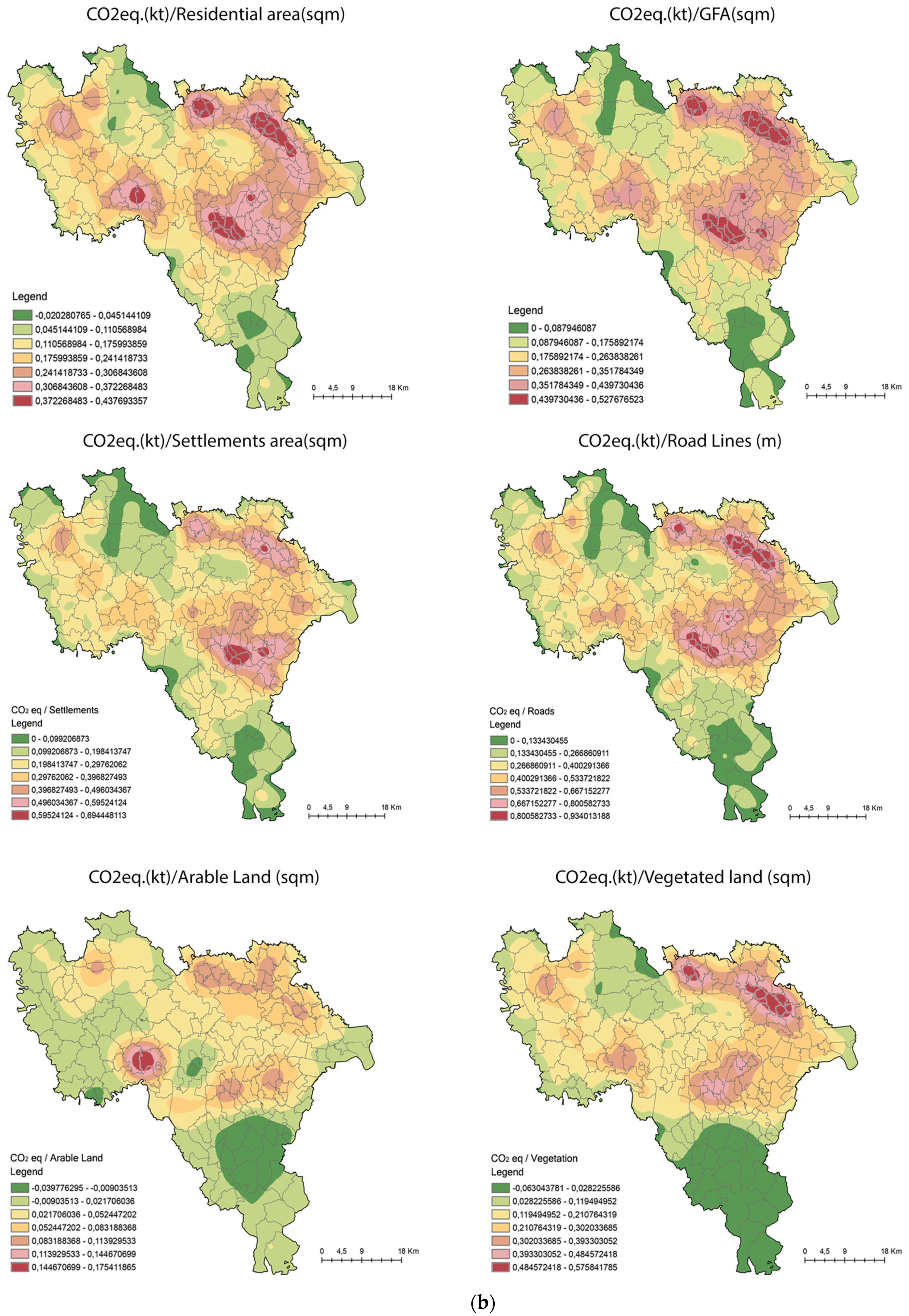
Figure 1b reveals that municipalities with a larger production area tend to have higher emissions. Similarly, for roads, the correlation is positive, but in the northern part of the province, areas with medium–high rates of emissions correspond to medium–high kilometers of roads, whereas in the southern part, areas with medium–high rates of roads correspond to fewer emissions. The agricultural area map is homogeneous, indicating that agriculture generally has a low contribution to emissions. As for vegetation, there is a high area dedicated to vegetation in the southern part and a low area in the northern part due to cultivation by agricultural soils.
3.1.3. Multiple Regression Analysis
From the indicators and related data presented in Section 2.2 and Section 2.3, the authors developed a multiple regression equation to link emissions data resulting from INEMAR algorithms and socio-demographic and territorial indicators. The objective is to establish a relationship of dependence of emissions (dependent variable Y) on socio-demographic, geographical, and territorial factors (independent variables X) through a multiple regression model. This model allows for the determination of the relationship (on average) between the independent variables , , …, and the dependent variable y through a linear relation [44,45,46].
where:
- intercept;
- inclination of y with respect to variable holding constant variables ,… ;
- : inclination of y with respect to variable holding constant variables , … .
The purpose of the following estimated regression models is to forecast the increase and decrease in the emissions from transport and residential installations based on changes in various indicators. Additionally, these models aim to identify which aspects are priorities in the planning and formulation process of policies and regulations.
The resulting estimated multiple regression model (6) is as follows:
The coefficients in a multiple regression model shall be considered as net regression coefficients. They measure the variation in the response variable Y at one of the explanatory variables when the others are constant [47,48,49,50].
Thanks to this equation, it is possible to calculate the value of CO2eq. present within the province of Pavia without referring to INEMAR algorithms. To verify the effectiveness of this formula, CO2eq. was calculated based on the indicator values, and the average of the obtained values is equal to the average of the CO2eq. values provided by INEMAR.
3.2. Spatial Autocorrelation
3.2.1. Moran’s I and Cluster Map
The Global Moran’s Index values obtained for all the ratios are greater than zero, suggesting positive autocorrelation or a highly clustered pattern. The results of the spatial autocorrelation tool indicate that the pattern of the CO2eq. ratio with each socio-demographic and territorial indicator, at each feature location, is clustered [51] as shown in Table 5. This result is validated by observing the p-values and z-scores. The p-value obtained is less than 0.05 (p < 0.05), rejecting the null hypothesis of randomness and independence in the data values. The z-score obtained is greater than 2.58 (z-score > 2.58) for all three years, indicating less than a 1% probability that the observed model is the result of a stochastic process.
Figure 2 shows the graphs generated by the software ESRI-ArcGIS®.
As a method of scientific visualization of the spatial autocorrelation Moran I in every municipality of the province of Pavia, the authors have chosen to use the technique of the cluster map [52,53]. Cluster analyses identify areas where elements are significantly grouped relative to random distribution, using techniques such as spatial clustering.
Figure 3a,b contain information on the spatial distribution of CO2 equivalent values compared to other demographic and territorial indicators, illustrating how these values are grouped or distributed within the province.
- Not Significant: There is no statistical evidence of significant spatial clustering in the data. In other words, there are no obvious spatial patterns that emerge from the analysis.
- High–High Cluster: A cluster of areas with a high CO2 equivalent value and high values of other demographic or territorial indicators. This means that the areas in this cluster have relatively high values for both variables.
- High–Low Outliers: Areas with high CO2 equivalent values but low values of other demographic or territorial indicators.
- Low–High Outliers: Areas with low CO2 equivalent values but high values of other demographic or territorial indicators.
- Low–Low Cluster: A cluster of areas with low CO2 equivalent values and low values of other demographic or territorial indicators. This means that the areas in this cluster have relatively low values for both variables.
In Figure 3a, the map CO2eq./ population mainly highlights two clusters: one LL in the area around the municipality of Pavia and one H-H to the west of the province, with blue municipalities indicating a low level of emissions compared to the population. In the map CO2eq./ density, two main clusters are evident: one LL to the east and one H-H to the west of the province, with red municipalities indicating a high CO2 value compared to the population density. In the map CO2eq./ GDP, mainly two clusters are highlighted: one LL to the east and one H-H to the west of the province. The map CO2eq./ territorial area shows an L-L cluster south of the province where the municipalities have fewer emissions than the territorial area, possibly due to the large presence of vegetation and the low presence of industrial settlements. In the maps CO2eq./ residential area and CO2eq./ GFA, two types of clusters are primarily identified: the cluster containing the municipalities LL and HL to the south of the province and the cluster containing the municipalities H-H and L-H to the west. In Figure 3b, the map CO2eq. highlights the relevant cluster to the west containing the municipalities H-H due to the large presence of industrial settlements in the area. In the map CO2eq./ road, the low level of roads in the southern part of the province is evident.
3.2.2. Kernel Density
The visualization of kernel density on ESRI-ArcGIS®, as shown in Figure 4a,b, provides a visual representation of the spatial distribution of point data, allowing for the identification and analysis of clusters or areas of high density of certain phenomena [40] within the province of Pavia. From the images, it can be noted that higher values are concentrated in the northeast area of the province, while lower values are in the south.
The maps shown are very similar to each other, and this confirms the positive correlation between emissions and the socio-demographic and territorial indicators considered. We see that the ratios are higher (and therefore a greater presence of emissions than the indicator considered) in the western area of the province, creating a semicircle around the city of Pavia.
4. Discussion
The research investigates the correlation between GHG emissions, in terms of the CO2 equivalent, and the key socio-demographic and territorial indicators in the province of Pavia. It recognizes the critical importance of understanding these dynamics for effective environmental and spatial management strategies. The complex interaction between emissions and changes in land use is crucial for mitigating their impacts on ecosystems and ensuring the long-term sustainability of human societies. The methods of analytic correlation and spatial autocorrelation highlight the positive correlation between GHG emissions (in terms of CO2 equivalent) and land use (in terms of socio-demographic and geographic and territorial indicators). Linear correlation is based on a direct linear relationship, while spatial correlation focuses on the spatial distribution of the data. The Spearman rank correlation coefficient reveals a significant non-linear correlation between CO2 equivalent emissions and several indicators, underscoring the diverse nature of the relationship. Moreover, the subsequent normalization of the data and recalculated Pearson correlation coefficients confirm the presence of exponential relationships, emphasizing the need for a nuanced understanding and modeling of these interactions. Spatial autocorrelation analysis using Moran’s index highlights a positive autocorrelation/clustering of high emissions areas, spatial heterogeneity, and localized hotspots of emissive areas. Figure 5 shows analogies and differences between the methods used in the paper.
5. Conclusions
The results underscore the need for holistic approaches to environmental management, emphasizing the importance of integrating socio-economic factors and spatial considerations into policy formulation and planning processes in the Province of Pavia. With this research, the authors presented an expeditious method to correlate spatial data on human macro-activities and greenhouse gas emissions. The results of this correlation can be used in several ways:
- To forecast emissions based on planning choices, which may concern the distribution of different urban functions within a municipality or the entire province under study.
- To identify areas that require further investigation, especially those elements that represent uniqueness and particular elements (L-L and H-H). This helps to highlight elements of punctual criticality that necessitate further examination.
- With these simplified formulas, it is possible to upscale to the whole national/regional territory. This allows for a first verification to validate the predicted results using the formulas in Table 4 on page 9 and to see if the study can be generalized to other territories outside the Italian context and then to other contexts around the world.
- The simplification of some algorithms that are otherwise very complex and require years of work is important for understanding the order of magnitude of the phenomena observed, particularly the emissions of greenhouse gases. These emissions are important worldwide mainly for macro values and not so much in specific detail, which is measured very precisely by INEMAR, which is the scientific data.
The aim of the authors is to find a direct and efficient method for calculating emissions based on indicators that are readily available through correlation and regression methods. Indeed, the algorithms of INEMAR are very complicated (for the common knowledge of sustainability scholars) and they require a high level of time consumption. The proposed methods can be easily implemented in all the contexts in which information about land use is available. Moreover, also considering the situation in which there is a lack of precise information about all human activities, starting from land use and basic information (such as for example GDP), the proposed method is useful to define the order of magnitude of the GHG’s emissions, with an acceptable approximation without introducing very complex modeling.
The methodology can be applied to many other contexts in which data and information about land use exist without any specific measure of GHG emissions. The presented methods cannot furnish exact final data, but they provide a negligible approximation that can be refined with the application in other contexts where all the data are available. The authors are confident that the process can lead to expeditious evaluations useful in environmental assessment processes such as, for example, Strategic Environmental Assessment.
The proposed simplified approach provides an effective method for assessing and predicting GHG’s emissions also in a future planning scenario, enabling better environmental consequences in certain regional planning decisions and more integrated relations among local decisions and potential global effects.
Supplementary Materials
The following supporting information can be downloaded at: https://www.mdpi.com/article/10.3390/air2020006/s1, Table S1: Data CO2eq., population, population density, GDP, territorial area residential area, GFA, settlements area, 3 road lines, arable land, vegetated land data of municipalities in Pavia Province.
Author Contributions
Conceptualization, R.D.L., R.B. and M.M.; methodology, R.B. and M.M.; software, M.M.; validation, R.B., R.D.L. and M.M.; formal analysis, R.B.; investigation, R.B.; resources, M.M.; data curation, R.B.; writing—original draft preparation, M.M.; writing—review and editing, R.D.L.; visualization, R.D.L.; supervision, R.D.L.; project administration, R.D.L.; funding acquisition, R.D.L. All authors have read and agreed to the published version of the manuscript.
Funding
This research received no external funding.
Institutional Review Board Statement
Not applicable.
Informed Consent Statement
Not applicable.
Data Availability Statement
ISTAT (National Institute of Statistics) Available online: https://www.istat.it/en/ (accessed on 2 February 2024). INEMAR (INventory of atmospheric emissions)—ARPA Lombardia Available online: https://www.inemar.eu/xwiki/bin/view/Inemar/ (accessed on 2 February 2024). Geoportale Lombardy Region. Available online: https://www.geoportale.regione.lombardia.it/download (accessed on 10 September 2023).
Conflicts of Interest
The authors declare no conflicts of interest.
References
- D’Odorico, P.; Davis, K.F.; Rosa, L.; Carr, J.A.; Chiarelli, D.; Dell’Angelo, J.; Rulli, M.C. The global food-energy-water nexus. Rev. Geophys. 2018, 56, 456–531. [Google Scholar]
- Beall, J.; Fox, S. Cities and Development, 1st ed.; Routledge: London, UK, 2009. [Google Scholar]
- Sathaye, J.; Shukla, P.R.; Ravindranath, N.H. Climate change, sustainable development and India: Global and national concerns. Curr. Sci. 2006, 90, 314–325. [Google Scholar]
- Young, O.R. The Institutional Dimensions of Environmental Change: Fit, Interplay, and Scale; MIT Press: Cambridge, MA, USA, 2002. [Google Scholar]
- Treweek, J. Ecological impact assessment. Impact Assess. 1995, 13, 289–315. [Google Scholar] [CrossRef]
- Babiy, A.P.; Kharytonov, M.M.; Gritsan, N.P. Connection between emissions and concentrations of atmospheric pollutants. In Air Pollution Processes in Regional Scale; Springer: Dordrecht, The Netherlands, 2003; pp. 11–19. [Google Scholar]
- Janssen, S.; Dumont, G.; Fierens, F.; Mensink, C. Spatial interpolation of air pollution measurements using CORINE land cover data. Atmos. Environ. 2008, 42, 4884–4903. [Google Scholar] [CrossRef]
- Xu, G.; Jiao, L.; Zhao, S.; Yuan, M.; Li, X.; Han, Y.; Zhang, B.; Dong, T. Examining the impacts of land use on air quality from a spatio-temporal perspective in Wuhan, China. Atmosphere 2016, 7, 62. [Google Scholar] [CrossRef]
- Zheng, S.; Zhou, X.; Singh, R.P.; Wu, Y.; Ye, Y.; Wu, C. The spatiotemporal distribution of air pollutants and their relationship with land-use patterns in Hangzhou city, China. Atmosphere 2017, 8, 110. [Google Scholar] [CrossRef]
- Bashir, M.F.; Jiang, B.; Komal, B.; Bashir, M.A.; Farooq, T.H.; Iqbal, N.; Bashir, M. Correlation between environmental pollution indicators and COVID-19 pandemic: A brief study in Californian context. Environ. Res. 2020, 187, 109652. [Google Scholar] [CrossRef]
- Zimmerman, N.; Li, H.Z.; Ellis, A.; Hauryliuk, A.; Robinson, E.S.; Gu, P.; Shah, R.U.; Ye, G.Q.; Snell, L.; Subramanian, R.; et al. Improving correlations between land use and air pollutant concentrations using wavelet analysis: Insights from a low-cost sensor network. Aerosol Air Qual. Res. 2020, 20, 314–328. [Google Scholar] [CrossRef]
- Hong, J.; Shen, Q. Residential density and transportation emissions: Examining the connection by addressing spatial autocorrelation and self-selection. Transp. Res. Part D Transp. Environ. 2013, 22, 75–79. [Google Scholar] [CrossRef]
- Heres-Del-Valle, D.; Niemeier, D. CO2 emissions: Are land-use changes enough for California to reduce VMT? Specification of a two-part model with instrumental variables. Transp. Res. Part B Methodol. 2011, 45, 150–161. [Google Scholar] [CrossRef]
- Wen, Y.; Wu, R.; Zhou, Z.; Zhang, S.; Yang, S.; Wallington, T.J.; Shen, W.; Tan, Q.; Deng, Y.; Wu, Y. A data-driven method of traffic emissions mapping with land use random forest models. Appl. Energy 2022, 305, 117916. [Google Scholar] [CrossRef]
- Feliciano, D.; Slee, B.; Hunter, C.; Smith, P. Estimating the contribution of rural land uses to greenhouse gas emissions: A case study of North East Scotland. Environ. Sci. Policy 2013, 25, 36–49. [Google Scholar] [CrossRef]
- Pezzagno, M.; Richiedei, A.; Tira, M. Spatial planning policy for sustainability: Analysis connecting land use and GHG emission in rural areas. Sustainability 2020, 12, 947. [Google Scholar] [CrossRef]
- De Lotto, R. Elementi della Città Flessibile; Maggioli Politecnica: Santarcangelo di Romagna, Italy, 2022. [Google Scholar]
- De Lotto, R. Flexibility in urban planning: Rules, opportunities and limits. In Cities and Communities across Europe: Governance Design for a Sustainable Future; Suárez, J.J.R.A., Ed.; ARANZADI/CIVITAS: Pamplona, Spain, 2023; pp. 93–112. [Google Scholar]
- Maranzano, P. Air quality in Lombardy, Italy: An overview of the environmental monitoring system of ARPA Lombardia. Earth 2022, 3, 172–203. [Google Scholar] [CrossRef]
- Caserini, S.; Giani, P.; Cacciamani, C.; Ozgen, S.; Lonati, G. Influence of climate change on the frequency of daytime temperature inversions and stagnation events in the Po Valley: Historical trend and future projections. Atmos. Res. 2017, 184, 15–23. [Google Scholar] [CrossRef]
- ISTAT (National Institute of Statistics). Available online: https://www.istat.it/en/ (accessed on 2 February 2024).
- Emission factors, I.N.E.M.A.R. Available online: https://www.inemar.eu/xwiki/bin/view/InemarDatiWeb/I+fattori+di+emissione (accessed on 2 February 2024).
- INEMAR (INventory of Atmospheric Emissions)—ARPA Lombardia. Available online: https://www.inemar.eu/xwiki/bin/view/Inemar/ (accessed on 2 February 2024).
- Wiggering, H.; Dalchow, C.; Glemnitz, M.; Helming, K.; Müller, K.; Schultz, A.; Zander, P. Indicators for multifunctional land use—Linking socio-economic requirements with landscape potentials. Ecol. Indic. 2006, 6, 238–249. [Google Scholar] [CrossRef]
- Esengulova, N.; Balena, P.; De Lucia, C.; Lopolito, A.; Pazienza, P. Key Drivers of Land Use Changes in the Rural Area of Gargano (South Italy) and Their Implications for the Local Sustainable Development. Land 2024, 13, 166. [Google Scholar] [CrossRef]
- Geoportale Lombardy Region. Available online: https://www.geoportale.regione.lombardia.it/download (accessed on 10 September 2023).
- Gogtay, N.J.; Thatte, U.M. Principles of correlation analysis. J. Assoc. Physicians India 2017, 65, 78–81. [Google Scholar] [PubMed]
- Senthilnathan, S. Usefulness of Correlation Analysis; 2019. SSRN 3416918. Available online: https://papers.ssrn.com/sol3/papers.cfm?abstract_id=3416918 (accessed on 2 February 2024).
- Myers, L.; Sirois, M.J. Spearman correlation coefficients, differences between. In Encyclopedia of Statistical Sciences; Wiley: Hoboken, NJ, USA, 2004; Volume 12. [Google Scholar]
- De Winter, J.C.; Gosling, S.D.; Potter, J. Comparing the Pearson and Spearman correlation coefficients across distributions and sample sizes: A tutorial using simulations and empirical data. Psychol. Methods 2016, 21, 273. [Google Scholar] [CrossRef]
- Bolboaca, S.D.; Jäntschi, L. Pearson versus Spearman, Kendall’s tau correlation analysis on structure-activity relationships of biologic active compounds. Leonardo J. Sci. 2006, 5, 179–200. [Google Scholar]
- Cohen, I.; Huang, Y.; Chen, J.; Benesty, J. Noise Reduction in Speech Processing; Springer: Berlin/Heidelberg, Germany, 2009; pp. 1–4. [Google Scholar]
- Thelwall, M. Interpreting correlations between citation counts and other indicators. Scientometrics 2016, 108, 337–347. [Google Scholar] [CrossRef]
- Anselin, L.; Syabri, I.; Kho, Y. GeoDa: An introduction to spatial data analysis. In Handbook of Applied Spatial Analysis: Software Tools, Methods and Applications; Fischer, M., Getis, A., Eds.; Springer: Berlin/Heidelberg, Germany, 2009; pp. 73–89. [Google Scholar]
- Murgante, B.; Scorza, F. Autocorrelazione Spaziale e Pianificazione del Territorio: Principi ed Applicazioni; Libria: Melfi, Italy, 2023. [Google Scholar]
- Cliff, A.D.; Ord, K. Spatial autocorrelation: A review of existing and new measures with applications. Econ. Geogr. 1970, 46, 269–292. [Google Scholar] [CrossRef]
- Chen, Y. Spatial autocorrelation equation based on Moran’s index. Sci. Rep. 2023, 13, 19296. [Google Scholar] [CrossRef] [PubMed]
- Krisp, J.M.; Špatenková, O. Kernel density estimations for visual analysis of emergency response data. In Geographic Information and Cartography for Risk and Crisis Management: Towards Better Solutions; Springer: Berlin/Heidelberg, Germany, 2010; pp. 395–408. [Google Scholar]
- Shi, X.; Alford-Teaster, J.; Onega, T. Kernel density estimation with geographically masked points. In Proceedings of the 17th International Conference on Geoinformatics, Fairfax, VA, USA, 12–14 August 2009. [Google Scholar]
- Milic, N.; Popovic, B.; Mijalkovic, S.; Marinkovic, D. The influence of data classification methods on predictive accuracy of kernel density estimation hotspot maps. Int. Arab J. Inf. Technol. 2019, 16, 1053–1062. [Google Scholar]
- Lucà, F.; Conforti, M.; Robustelli, G. Comparison of GIS-based gullying susceptibility mapping using bivariate and multivariate statistics: Northern Calabria, South Italy. Geomorphology 2011, 134, 297–308. [Google Scholar] [CrossRef]
- Speich, M.J.; Bernhard, L.; Teuling, A.J.; Zappa, M. Application of bivariate mapping for hydrological classification and analysis of temporal change and scale effects in Switzerland. J. Hydrol. 2015, 523, 804–821. [Google Scholar] [CrossRef]
- Fabrizio, E.; Garnero, G. Analisi di visibilità con tecniche GIS per la valutazione paesistica. In Proceedings of the L’edilizia Rurale Tra Sviluppo Tecnologico e Tutela del Territorio. Convegno della II Sezione AIIA, Florence, Italy, 20–22 September 2012. [Google Scholar]
- Song, Y.; Kang, L.; Lin, F.; Sun, N.; Aizezi, A.; Yang, Z.; Wu, X. Estimating the spatial distribution of soil heavy metals in oil mining area using air quality data. Atmos. Environ. 2022, 287, 119274. [Google Scholar] [CrossRef]
- Kleine Deters, J.; Zalakeviciute, R.; Gonzalez, M.; Rybarczyk, Y. Modeling PM 2.5 urban pollution using machine learning and selected meteorological parameters. J. Electr. Comput. Eng. 2017, 2017, 5106045. [Google Scholar]
- Del Giudice, V. L’analisi di regressione multipla nella stima “per valori tipici” in, C.e.S.E.T. Aspetti evolutivi della scienza estimativa. In Seminario in Onore di Ernesto Marenghi; Firenze University Press: Florence, Italy, 1995; pp. 1–10. [Google Scholar]
- Negri, I. Regressione multipla. In Probabilità e Statistica per L’ingegneria e le Scienze; McGraw Hill: New York, NY, USA, 2006; pp. 420–433. [Google Scholar]
- Berry, W.D.; Feldman, S.; Stanley Feldman, D. Multiple Regression in Practice (No. 50). 1985; Available online: https://www.worldcat.org/title/multiple-regression-in-practice/oclc/12279592 (accessed on 2 February 2024).
- Irwin, J.R.; McClelland, G.H. Misleading heuristics and moderated multiple regression models. J. Mark. Res. 2001, 38, 100–109. [Google Scholar] [CrossRef]
- Nordio, F.; Kloog, I.; Coull, B.A.; Chudnovsky, A.; Grillo, P.; Bertazzi, P.A.; Schwartz, J. Estimating spatio-temporal resolved PM10 aerosol mass concentrations using MODIS satellite data and land use regression over Lombardy, Italy. Atmos. Environ. 2013, 74, 227–236. [Google Scholar] [CrossRef]
- Kumari, M.; Sarma, K.; Sharma, R. Using Moran’s I and GIS to study the spatial pattern of land surface temperature in relation to land use/cover around a thermal power plant in Singrauli district, Madhya Pradesh, India. Remote Sens. Appl. Soc. Environ. 2019, 15, 100239. [Google Scholar] [CrossRef]
- Zhang, C.Y.; Zhao, L.; Zhang, H.; Chen, M.N.; Fang, R.Y.; Yao, Y.; Zhang, Q.P.; Wang, Q. Spatial-temporal characteristics of carbon emissions from land use change in Yellow River Delta region, China. Ecol. Indic. 2022, 136, 108623. [Google Scholar] [CrossRef]
- Ding, H.; Shi, W. Land-use/land-cover change and its influence on surface temperature: A case study in Beijing City. Int. J. Remote Sens. 2013, 34, 5503–5517. [Google Scholar] [CrossRef]
Figure 1.
(a) Bivariate map CO2eq. and population–population density–GDP–territorial area–residential area–GFA. (b) Bivariate map CO2eq. and settlements area–road lines–arable land–vegetated land.
Figure 1.
(a) Bivariate map CO2eq. and population–population density–GDP–territorial area–residential area–GFA. (b) Bivariate map CO2eq. and settlements area–road lines–arable land–vegetated land.


Figure 2.
Moran I graph.


Figure 3.
(a) Clustered map ratio between CO2eq. and population–population density–GDP–territorial area. (b) Clustered map ratio between CO2eq. and residential area–GFA–settlements area–road lines–arable land–vegetated land.
Figure 3.
(a) Clustered map ratio between CO2eq. and population–population density–GDP–territorial area. (b) Clustered map ratio between CO2eq. and residential area–GFA–settlements area–road lines–arable land–vegetated land.


Figure 4.
(a) Kernel density map ratio between CO2eq. and population–population density–GDP–territorial area–residential area–GFA. (b) Kernell density map ratio between CO2eq. and settlements area–road lines–arable land–vegetated land.
Figure 4.
(a) Kernel density map ratio between CO2eq. and population–population density–GDP–territorial area–residential area–GFA. (b) Kernell density map ratio between CO2eq. and settlements area–road lines–arable land–vegetated land.


Figure 5.
Analogies and differences between Pearson’s correlation, Spearman’s rank correlation, Moran’s spatial autocorrelation, and Kernel density.
Figure 5.
Analogies and differences between Pearson’s correlation, Spearman’s rank correlation, Moran’s spatial autocorrelation, and Kernel density.


Table 1.
Environmental, socio-demographic, and territorial indicators for each municipality.
| Municipality | CO2eq. [kt/year] | Population [inhab.] | Population Density [inhab./sqkm] | GDP [EUR] | Territorial Area [sqkm] | Residential Area [sqm] | GFA [mq] | Settlements Area [sqm] | Road Lines [m] | Arable Land [sqm] | Vegetated Area [sqm] |
|---|---|---|---|---|---|---|---|---|---|---|---|
| Ferrera Erbognone | 2870 | 1171 | 59.9 | 15,442,841.00 | 19.17 | 517,337 | 667,532 | 2,438,116 | 43,778 | 14,728,155 | 1,295,014 |
| Sannazzaro de’ Burgondi | 2245 | 5533 | 237.3 | 77,957,469.00 | 23.33 | 1,385,716 | 1,429,065 | 2,120,149 | 78,233 | 16,561,204 | 1,886,223 |
| Voghera | 886 | 39,356 | 621.9 | 637,341,042.00 | 63.44 | 7,261,991 | 6,785,758 | 3,556,511 | 274,498 | 48,037,718 | 2,467,872 |
| Pavia | 351 | 71,297 | 1134.2 | 1,502,659,302.00 | 63.25 | 8,983,402 | 10,776,269 | 4,734,546 | 346,757 | 38,550,845 | 7,294,540 |
| Vigevano | 287 | 63,268 | 768 | 970,129,252.00 | 81.36 | 10,876,712 | 8,962,370 | 4,413,324 | 434,552 | 43,620,466 | 18,250,505 |
| Verretto | 2 | 402 | 147.3 | 4,957,052.00 | 2.71 | 194,653 | 96,498 | 128,278 | 11,439 | 2,031,408 | 327,641 |
| Golferenzo | 2 | 196 | 45.1 | 2,804,711.00 | 4.42 | 224,208 | 91,058 | 20,452 | 27,638 | 2,992,303 | 1,118,606 |
| Rea | 1.5 | 431 | 145.6 | 5,745,015.00 | 2.16 | 202,116 | 163,207 | 83,606 | 12,558 | 1,313,383 | 234,622 |
| Lirio | 1.56 | 130 | 75.1 | 1,324,318.00 | 1.75 | 130,811 | 59,931 | 22,973 | 11,928 | 1,347,821 | 193,722 |
| Calvignano | 1 | 127 | 18.4 | 1,206,421.00 | 6.98 | 209,447 | 667,532 | 17,173 | 27,830 | 4,600,624 | 1,962,481 |
Table 2.
Spearman rank correlation coefficient between environmental, socio-demographic, and territorial indicators in the province of Pavia.
Table 2.
Spearman rank correlation coefficient between environmental, socio-demographic, and territorial indicators in the province of Pavia.
| Correlation | Population [inhab.] | Population Density [inhab/sqkm] | GDP [EUR] | Territorial Area [sqkm] | Residential Area [sqkm] | GFA [sqm] | Settlements Area [sqm] | Road Lines [m] | Arable Land [sqm] | Vegetated Land [sqm] |
|---|---|---|---|---|---|---|---|---|---|---|
| CO2eq. | 0.750 | 0.383 | 0.727 | 0.631 | 0.713 | 0.779 | 0.790 | 0.488 | 0.760 | 0.241 |
Table 3.
Pearson correlation coefficient between environmental, socio-demographic, and territorial indicators in the province of Pavia.
Table 3.
Pearson correlation coefficient between environmental, socio-demographic, and territorial indicators in the province of Pavia.
| Correlation | Population [inhabitants] | Population Density [inhab/skmq] | GDP [EUR] | Territorial Area [kmq] | Residential Area [mq] | GFA [mq] | Settlements Area [mq] | Road Lines [m] | Arable Land [mq] | Vegetated Land [mq] |
|---|---|---|---|---|---|---|---|---|---|---|
| CO2eq. | 0.726 | 0.396 | 0.704 | 0.614 | 0.634 | 0.773 | 0.782 | 0.504 | 0.707 | 0.194 |
Table 4.
Equations between CO2eq. and socio-demographic and territorial indicators.
| Dependent Variable y | Independent Variable x | Equation |
|---|---|---|
| CO2eq. | Population | |
| GDP | ||
| Territorial Area | ||
| Residential Area | ||
| GFA | ||
| Settlements Area | ||
| Road Lines | ||
| Arable Land | ||
| Vegetated land |
Table 5.
Moran’s Index between ratio between CO2eq. and socio-demographic and territorial indicators in the province of Pavia.
Table 5.
Moran’s Index between ratio between CO2eq. and socio-demographic and territorial indicators in the province of Pavia.
| Correlation | CO2eq./Population | CO2eq./Population Density | CO2eq./GDP | CO2eq./Territorial Area | CO2eq./Residential Area | CO2eq./GFA | CO2eq./Settlement Area | CO2eq./Road Lines | CO2eq./Arable Land | Co2eq./Vegetated Land |
|---|---|---|---|---|---|---|---|---|---|---|
| Moran I | 0.726 | 0.396 | 0.704 | 0.614 | 0.634 | 0.773 | 0.782 | 0.504 | 0.707 | 0.194 |
Disclaimer/Publisher’s Note: The statements, opinions and data contained in all publications are solely those of the individual author(s) and contributor(s) and not of MDPI and/or the editor(s). MDPI and/or the editor(s) disclaim responsibility for any injury to people or property resulting from any ideas, methods, instructions or products referred to in the content. |
© 2024 by the authors. Licensee MDPI, Basel, Switzerland. This article is an open access article distributed under the terms and conditions of the Creative Commons Attribution (CC BY) license (https://creativecommons.org/licenses/by/4.0/).
Share and Cite
MDPI and ACS Style
De Lotto, R.; Bellati, R.; Moretti, M. Correlation Methodologies between Land Use and Greenhouse Gas emissions: The Case of Pavia Province (Italy). Air 2024, 2, 86-108. https://doi.org/10.3390/air2020006
AMA Style
De Lotto R, Bellati R, Moretti M. Correlation Methodologies between Land Use and Greenhouse Gas emissions: The Case of Pavia Province (Italy). Air. 2024; 2(2):86-108. https://doi.org/10.3390/air2020006
Chicago/Turabian StyleDe Lotto, Roberto, Riccardo Bellati, and Marilisa Moretti. 2024. "Correlation Methodologies between Land Use and Greenhouse Gas emissions: The Case of Pavia Province (Italy)" Air 2, no. 2: 86-108. https://doi.org/10.3390/air2020006