Time Domain Vibration Analysis of Cracked Ice Shelf

Abstract

Understanding the effect of cracks on ice shelf vibrations is crucial for assessing their structural integrity, predicting possible breakup events, and understanding their interactions with the surrounding environment. In this work, a novel approach to modelling the simulation of cracked ice shelf vibrations using thin beam approximation along with cracked beam boundary conditions is proposed. A simplified model was used in which the ice shelf was modelled as a thin elastic plate floating on water of a constant depth. The crack was modelled as a connected spring condition, a model which is standard in other fields but which has not been applied to ice shelves. The boundary conditions assumed that there was no flow of energy into the open water, and two possible boundary conditions were considered: no pressure and no flux. The focus of this work is to show how we can simulate the motion of an ice shelf with a crack, and this is the first step towards modelling the effect of crack and crack propagation on ice shelf breakup.

1. Introduction

Ice shelves are large floating platforms of ice that extend from the edge of continental ice sheets into the ocean. They play a crucial role in the dynamics of polar regions and have significant impacts on global sea level rises. Recent studies of Antarctica show that changes in the Antarctic coastline, such as melting ice shelves and glacier retreat, can have significant implications for global sea level rises and climate patterns [1,2]. In the Antarctic region, ice shelves serve as vital habitats for various species, including Emperor penguins, which rely on ice shelves for safety and breeding grounds. In 2016, in Halley Bay, more than 10,000 penguin chicks vanished due to an intense storm that broke the sea ice before the chicks had matured [3]. In February 2019, a rift spanning most of the Brunt Ice Shelf in Antarctica appeared ready to spawn an iceberg about twice the size of New York City. According to the British Antarctic Survey (BAS), the break occurred late on 22 January 2023, and produced a new iceberg with an area of 1550 square kilometres [4,5,6].

Ice shelves are vulnerable to environmental changes, particularly those associated with climate change. Rising temperatures, changes in ocean currents, and increased melting can weaken ice shelves, making them more susceptible to breakup events [2]. Understanding the mechanisms and impacts of the breakup of ice shelves is essential to predict future changes in the polar regions, assess the risks associated with climate change, and develop strategies to mitigate its effects. Ice shelves are dynamic structures that respond to external forces, such as ocean currents, atmospheric pressure, and tidal forces. Understanding the factors that contribute to the vibration of ice shelves (which we define as changes in strain that occur in the order of minutes to seconds in which the strain oscillates about a reference value) is essential to predict their stability and assess the risk of disintegration. Studying the breakup of ice shelves is important because of their significant role in the Earth’s climate system, sea level rises, and the stability of polar regions [7].

Seismic data collected from Antarctic ice shelves and ice tongues indicate that these structures oscillate due to ocean surface waves, with evidence that the vibrations travel as flexural waves. The ocean waves responsible for inducing these vibrations vary from frequent long-period swells, which are observed in summer when the sea ice barrier surrounding the shelves is minimal or nonexistent, to occasional infragravity and tsunami waves. There is substantial evidence suggesting that these vibrations lead to icequakes and the significant calving of icebergs and that they can even initiate catastrophic disintegration events [8,9]. There is extensive exerimental literature showing the vibration of ice shelves [10,11]. The study of ice shelf vibration was first established by Holdsworth and Glynn [12], who investigated the dynamic behaviour of ice shelves in response to oceanic tides and atmospheric pressure variations. They used thin beam approximation to calculate ice shelf vibration which based on the early work of [13]. Different solution methods have been used to determine the vibration of ice shelves. In [14,15], ice shelves were treated as a thin elastic plate (or beam since the problem was two-dimensional) that floated on an ocean surface with a uniform depth, and they used the Euler–Bernoulli beam theory and the shallow-water equation. This very simple model has been extended by subsequent researchers using the finite element method [16,17] and complex analytic methods [18] to predict the vibrations of ice shelves. Recently, extensive work has been conducted using thin plate and shallow water approximation [19,20], with extensions to include compression waves [21].

There is extensive engineering literature on cracks in beams that can be applied to cracked ice shelves under standard modelling assumptions. In [22], a theory for the lateral vibration of a cracked Euler–Bernoulli beam with open single-edge or double-edge cracks was developed. In [23,24], researchers measured the natural frequencies of cracked beams and used the Euler–Bernoulli theory to obtain a closed-form solution. Other studies [25,26,27] have used finite element methods to address the vibration of cracked beams, while in [28], spatial wavelet analysis was used to detect the location and size of cracked beams.

In this paper, a crack in an ice shelf was modelled using the crack beam boundary conditions of [29] together with the flux and pressure conditions discussed in [30]. We employed shallow water approximation in which the fluid was assumed to have a uniform, horizontal velocity. This assumption is standard [15] and applies for long-period vibrations, such as those considered here. We calculated the modes of vibration and conducted a time-dependent simulation of a cracked ice shelf using these modes of vibration. The purpose of this work is to show that it is possible to model the effect of a crack in an ice shelf and simulate the motion in the time domain. From this, time domain simulation models that allow for crack growth or propagation can be developed.

2. Mathematical Model

In this model, we folloedw the work of [14,19] in modelling the vibration of an ice shelf floating on shallow water. The ice shelf was assumed to be free at the open water end and clamped at the landward end. Following [14,19], again, we assumed that the ice shelf and the water remained in contact at all points $x\in [0,L]$, where $x=0$ is the landward end and $x=L$ is the seaward end.

By the assumption of linear water wave theory, the water velocity was defined by the potential function $\varphi$. The potential $\varphi$ satisfied the linear shallow water equation [31]:

$${\displaystyle \frac{{\partial }^2\varphi }{\partial x^2}}=-{\displaystyle \frac{1}{H}}{\displaystyle \frac{\partial \eta }{\partial t}}.$$

(1)

where t denotes time, $\eta$ is the vertical displacement of the lower surface of the ice, and H is the uniform depth of the water. Following the work of [19], we considered two assumptions. The first one was the standard assumption with no-flux conditions at the ends of the cavity. This meant that

$${\displaystyle \frac{\partial \Phi }{\partial x}}=0,\mathrm{at}x=0,L.$$

(2)

The second assumption was that the pressure at the seaward end was zero, that is

$$\begin{array}{c}\hfill {\displaystyle \frac{\partial \Phi }{\partial x}}=0,\mathrm{at}x=0,\\ \hfill \Phi =0,\mathrm{at}x=L.\end{array}$$

(3)

To determine the flexure of an ice shelf, thin beam approximation was used to drive the following equation:

$$D{\displaystyle \frac{{\partial }^4\eta }{\partial x^4}}+{\rho }_{i}h{\displaystyle \frac{{\partial }^2\eta }{\partial t^2}}+{\rho }_{w}g\eta =-{\rho }_w{\displaystyle \frac{\partial \varphi }{\partial t}}.$$

(4)

Here, $D={\displaystyle \frac{E{h}^3}{12(1-v^2)}}$ is the flexural rigidity of the shelf, where $E=11$ GPa is its effective Young’s modulus and $v=0.33$ is its Poisson’s ratio. The density of the ice ${\rho }_i=922.5{\mathrm{kgm}}^{-3}$, the density of the water ${\rho }_w=1024{\mathrm{kgm}}^{-3}$, and $g=9.81{\mathrm{ms}}^{-2}$ is the acceleration of gravity. We note here that there is great variation in ice shelf lengths and thicknesses and that we were able in this work to only simulate a very small subset of values. We also note that the value of the Young’s modulus for an ice shelf remains only an estimate. The boundary conditions for the clamped free ice shelf were the following:

For the clamped end where $x=0$, the conditions were

$$\eta =0,\mathrm{and}{\displaystyle \frac{\partial \eta }{\partial x}}=0,\mathrm{at}x=0,$$

(5)

For the free end where $x=L$, the conditions were

$${\displaystyle \frac{{\partial }^2\eta }{\partial x^2}}=0,\mathrm{and}{\displaystyle \frac{{\partial }^3\eta }{\partial x^3}}=0,\mathrm{at}x=L.$$

(6)

Following [14,32], a non-dimensionalisation was applied where

$$\widehat{x}={\displaystyle \frac{x}{L_c}}\mathrm{and}\widehat{t}={\displaystyle \frac{t}{t_c}}$$

(7)

where

$$L_c=\sqrt[4]{{\displaystyle \frac{D}{{\rho }_{w}g}}}\mathrm{and}{t}_c=\sqrt{{\displaystyle \frac{{\rho }_w{L}_c^6}{DH}}}$$

(8)

By combining a non-dimensional version of Equations (1) and (4) into a single governing equation by eliminating the displacement $\eta$, we obtained

$${\displaystyle \frac{{\partial }^6\varphi }{\partial x^6}}+M{\displaystyle \frac{{\partial }^4\varphi }{\partial t^2\partial x^2}}+{\displaystyle \frac{{\partial }^2\varphi }{\partial x^2}}-{\displaystyle \frac{{\partial }^2\varphi }{\partial t^2}}=0.$$

(9)

For clarity, the hats were dropped during the solution methods. Equation (9) depended on the single parameter

$$M={\displaystyle \frac{{\rho }_{i}hH}{{\rho }_w{L}_c^2}},$$

(10)

where $M\ll 1$. The time-harmonic solution of Equation (9) was as follows:

$$\Phi =Re\left\{X\left(x\right)e^{-i\omega t}\right\}.$$

(11)

In addition, Equation (9) became

$${\displaystyle \frac{{\partial }^{6}X}{\partial x^6}}+(1-M{\omega }^2){\displaystyle \frac{{\partial }^{2}X}{\partial x^2}}+{\omega }^{2}X=0,$$

(12)

Now, since we were dealing with a cracked ice shelf, the general solution was in the form of

$$X\left(x^{+}\right)=\sum _{n=1}^6{c}_n{e}^{k_{n}x},\mathrm{and}X\left(x^{-}\right)=\sum _{n=1}^6{d}_n{e}^{k_{n}x}.$$

(13)

Here, $X\left(x^{+}\right)$ is the solution for the right side of the crack where $x>S$ and $X\left(x^{-}\right)$ is the solution for the left side where $x<S$ where S is the location of the crack.

• $k_n$ are the roots of k of the characteristic polynomial:

  $$k^6+(1-M{\omega }^2)k^2+{\omega }^2=0.$$

  (14)

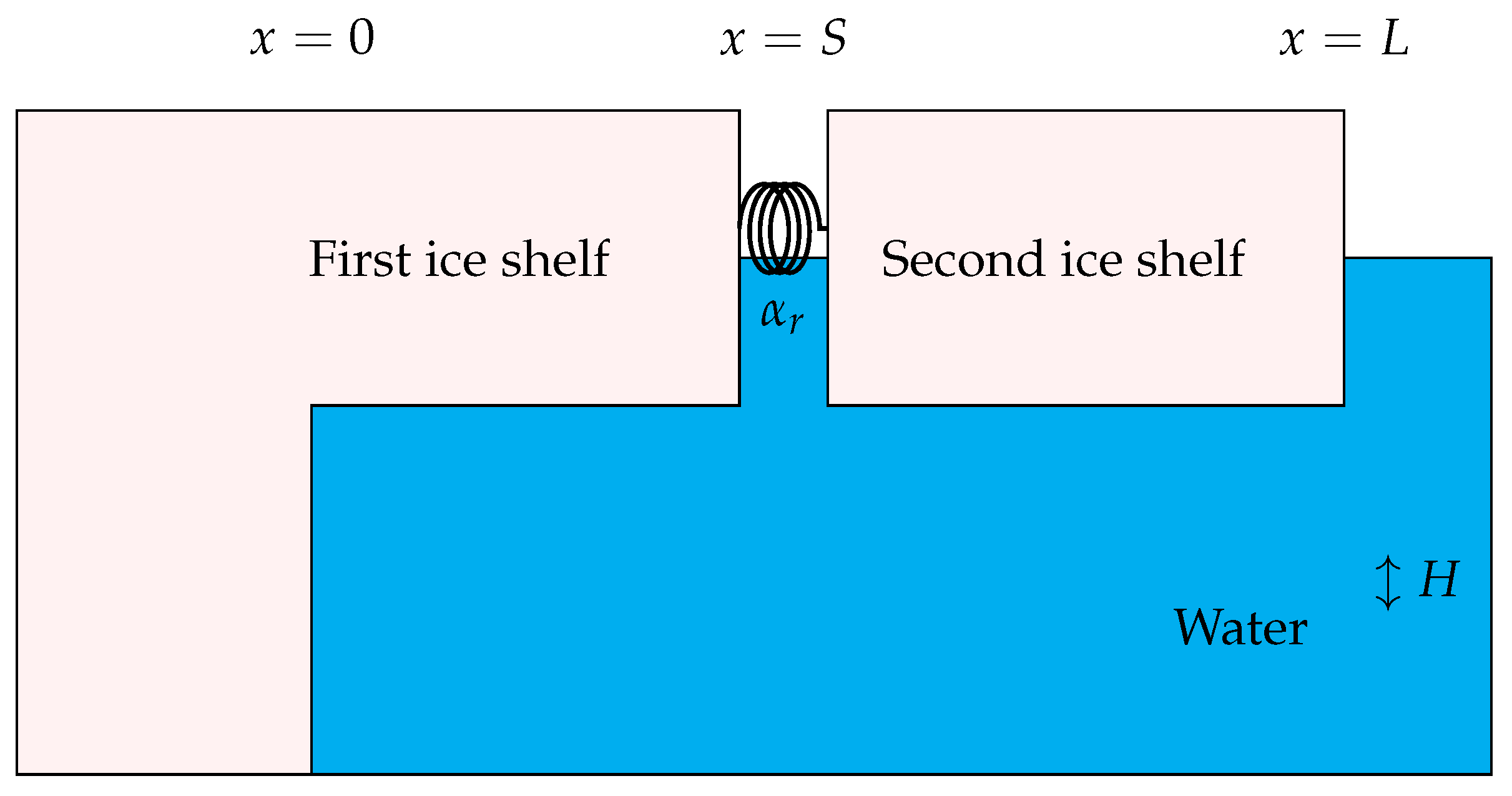
A schematic diagram of the cracked ice shelf is shown in Figure 1.

For the cracked ice shelf, we had six boundary conditions (three for each side of the ice shelf end) and six at the crack location. Thus, we had twelve unknowns and twelve homogeneous boundary conditions. At the open end, we had two possible boundary conditions. The no-flux condition meant that the fluid could not flow out from the seaward end of the ice shelf. Thus, the boundary conditions were as follows:

$$X^{\prime }\left(x^{-}\right)=0,X^{″}\left(x^{-}\right)=0\mathrm{and}{X}^{‴}\left(x^{-}\right)=0\mathrm{at}x=0,$$

(15)

$$X^{\prime }\left(x^{+}\right)=0,X^{\prime \prime \prime \prime }\left(x^{+}\right)=0\mathrm{and}{X}^{\prime \prime \prime \prime \prime }\left(x^{+}\right)=0\mathrm{at}x=L.$$

(16)

At the crack location, the conditions were [23,24]

$$X\left(x^{+}\right)=X\left(x^{-}\right),\mathrm{at}x=S.$$

(17)

$$X^{\prime }\left(x^{+}\right)=X^{\prime }\left(x^{-}\right),\mathrm{at}x=S.$$

(18)

$$X^{″}\left(x^{+}\right)=X^{″}\left(x^{-}\right),\mathrm{at}x=S.$$

(19)

$$X^{\prime \prime \prime \prime }\left(x^{+}\right)=X^{\prime \prime \prime \prime }\left(x^{-}\right),\mathrm{at}x=S.$$

(20)

$$X^{\prime \prime \prime \prime \prime }\left(x^{+}\right)=X^{\prime \prime \prime \prime \prime }\left(x^{-}\right),\mathrm{at}x=S.$$

(21)

$$X^{‴}\left(x^{+}\right)+{\displaystyle \frac{\lambda }{\alpha }}{X}^{\prime \prime \prime \prime }\left(x^{+}\right)=X^{‴}\left(x^{-}\right),\mathrm{at}x=S.$$

(22)

Here, $\lambda$ is equal to ${({\omega }^2\rho A{L}^4/EI)}^{1/4}$, $\alpha ={\alpha }_{r}L/EI$ is the non-dimensional stiffness of the rotational spring representing the crack, and S is the normalised crack location [23,24].

E is the Young’s modulus, I is the moment of inertia, A is the cross-sectional area, ${\rho }_i$ is the density of the ice, and $\omega$ is the angular frequency.

Spring stiffness ${\alpha }_r$ could be calculated from the following formula [29]:

$${\alpha }_r={\displaystyle \frac{EI}{5.346hf(a/h)}}.$$

where a and h are crack depth and ice thickness and $f(a/h)$ is the local compliance function calculated from the strain energy density function, which is discussed in detail in [23,24,29]. A schematic diagram for modelling the crack in the ice shelf as rotational spring is shown in Figure 2.

The twelve boundary conditions for the cracked ice shelf led to a system of twelve linear equations: please confirm if the bold format for variables should be kept? if possible, please unify the format throughout the whole paper. $\mathbf{Ac}=\mathbf{0}$. The matrix was as follows:

$$\left[\begin{array}{cccccccccccc}{k}_1& k_2& k_3& k_4& k_5& k_6& 0& 0& 0& 0& 0& 0\\ k_1^2& k_2^2& k_3^2& k_4^2& k_5^2& k_6^2& 0& 0& 0& 0& 0& 0\\ k_1^3& k_2^3& k_3^3& k_4^3& k_5^3& k_6^3& 0& 0& 0& 0& 0& 0\\ 0& 0& 0& 0& 0& 0& k_1{e}^{k_{1}L}& k_2{e}^{k_{2}L}& k_3{e}^{k_{3}L}& k_4{e}^{k_{4}L}& k_5{e}^{k_{5}L}& k_6{e}^{k_{6}L}\\ 0& 0& 0& 0& 0& 0& k_1^4{e}^{k_{1}L}& k_2^4{e}^{k_{2}L}& k_3^4{e}^{k_{3}L}& k_4^4{e}^{k_{4}L}& k_5^4{e}^{k_{5}L}& k_6^4{e}^{k_{6}L}\\ 0& 0& 0& 0& 0& 0& k_1^5{e}^{k_{1}L}& k_2^5{e}^{k_{2}L}& k_3^5{e}^{k_{3}L}& k_4^5{e}^{k_{4}L}& k_5^5{e}^{k_{5}L}& k_6^5{e}^{k_{6}L}\\ e^{k_{1}S}& e^{k_{2}S}& e^{k_{3}S}& e^{k_{4}S}& e^{k_{5}S}& e^{k_{6}S}& -e^{k_{1}S}& -e^{k_{2}S}& -e^{k_{3}S}& -e^{k_{4}S}& -e^{k_{5}S}& -e^{k_{6}S}\\ k_1{e}^{k_{1}S}& k_2{e}^{k_{2}S}& k_3{e}^{k_{3}S}& k_4{e}^{k_{4}S}& k_5{e}^{k_{5}S}& k_6{e}^{k_{6}S}& -k_1{e}^{k_{1}S}& -k_2{e}^{k_{2}S}& -k_3{e}^{k_{3}S}& -k_4{e}^{k_{4}S}& -k_5{e}^{k_{5}S}& -k_6{e}^{k_{6}S}\\ k_1^2{e}^{k_{1}S}& k_2^2{e}^{k_{2}S}& k_3^2{e}^{k_{3}S}& k_4^2{e}^{k_{4}S}& k_5^2{e}^{k_{5}S}& k_6^2{e}^{k_{6}S}& -k_1^2{e}^{k_{1}S}& -k_2^2{e}^{k_{2}S}& -k_3^2{e}^{k_{3}S}& -k_4^2{e}^{k_{4}S}& -k_5^2{e}^{k_{5}S}& -k_6^2{e}^{k_{6}S}\\ k_1^4{e}^{k_{1}S}& k_2^4{e}^{k_{2}S}& k_3^4{e}^{k_{3}S}& k_4^4{e}^{k_{4}S}& k_5^4{e}^{k_{5}S}& k_6^4{e}^{k_{6}S}& -k_1^4{e}^{k_{1}S}& -k_2^4{e}^{k_{2}S}& -k_3^4{e}^{k_{3}S}& -k_4^4{e}^{k_{4}S}& -k_5^4{e}^{k_{5}S}& -k_6^4{e}^{k_{6}S}\\ k_1^5{e}^{k_{1}S}& k_2^5{e}^{k_{2}S}& k_3^5{e}^{k_{3}S}& k_4^5{e}^{k_{4}S}& k_5^5{e}^{k_{5}S}& k_6^5{e}^{k_{6}S}& -k_1^5{e}^{k_{1}S}& -k_2^5{e}^{k_{2}S}& -k_3^5{e}^{k_{3}S}& -k_4^5{e}^{k_{4}S}& -k_5^5{e}^{k_{5}S}& -k_6^5{e}^{k_{6}S}\\ K_m& K_m& K_m& K_m& K_m& K_m& -k_1^3{e}^{k_{1}S}& -k_2^3{e}^{k_{2}S}& -k_3^3{e}^{k_{3}S}& -k_4^3{e}^{k_{4}S}& -k_5^3{e}^{k_{5}S}& -k_6^3{e}^{k_{6}S}\end{array}\right]\times \left[\begin{array}{c}c1\\ c2\\ c3\\ c4\\ c5\\ c6\\ d1\\ d2\\ d3\\ d4\\ d5\\ d6\end{array}\right]=0.$$

where $K_m=k_m^3{e}^{k_{m}S}+{\displaystyle \frac{\lambda }{\alpha }}{k}_m^4{e}^{k_{m}S}$, ($m=1,...,6)$.

From this matrix, we could find the value of $\omega$ that made $\mathrm{A}\left(\omega \right)$ singular. To do this, we needed to solve it numerically and search for the values of $\omega$ that made $\det \left(\mathrm{A}\right)=0$ or nearly zero. After we found the correct angular frequency ${\omega }_n$, we were able to find the coefficients $c_n$ and $d_n$ from the eigenvector associated with the zero eigenvalue. However, in practice, to find the mode shape or plot the simulation for the cracked ice shelf, we needed to adjust the matrix since we could see that on the right-hand side, the matrix contained rapidly growing exponential functions. These growing terms made the calculation unstable. Thus, we needed to stabilise the matrix by multiplying the $c_n$ and $d_n$ vectors by an exponential function as follows:

$$\left[\begin{array}{cccccccccccc}{k}_1& k_2& k_3& k_4& k_5& k_6& 0& 0& 0& 0& 0& 0\\ k_1^2& k_2^2& k_3^2& k_4^2& k_5^2& k_6^2& 0& 0& 0& 0& 0& 0\\ k_1^3& k_2^3& k_3^3& k_4^3& k_5^3& k_6^3& 0& 0& 0& 0& 0& 0\\ 0& 0& 0& 0& 0& 0& k_1{e}^{k_{1}L}& k_2{e}^{k_{2}L}& k_3{e}^{k_{3}L}& k_4{e}^{k_{4}L}& k_5{e}^{k_{5}L}& k_6{e}^{k_{6}L}\\ 0& 0& 0& 0& 0& 0& k_1^4{e}^{k_{1}L}& k_2^4{e}^{k_{2}L}& k_3^4{e}^{k_{3}L}& k_4^4{e}^{k_{4}L}& k_5^4{e}^{k_{5}L}& k_6^4{e}^{k_{6}L}\\ 0& 0& 0& 0& 0& 0& k_1^5{e}^{k_{1}L}& k_2^5{e}^{k_{2}L}& k_3^5{e}^{k_{3}L}& k_4^5{e}^{k_{4}L}& k_5^5{e}^{k_{5}L}& k_6^5{e}^{k_{6}L}\\ e^{k_{1}S}& e^{k_{2}S}& e^{k_{3}S}& e^{k_{4}S}& e^{k_{5}S}& e^{k_{6}S}& -e^{k_{1}S}& -e^{k_{2}S}& -e^{k_{3}S}& -e^{k_{4}S}& -e^{k_{5}S}& -e^{k_{6}S}\\ k_1{e}^{k_{1}S}& k_2{e}^{k_{2}S}& k_3{e}^{k_{3}S}& k_4{e}^{k_{4}S}& k_5{e}^{k_{5}S}& k_6{e}^{k_{6}S}& -k_1{e}^{k_{1}S}& -k_2{e}^{k_{2}S}& -k_3{e}^{k_{3}S}& -k_4{e}^{k_{4}S}& -k_5{e}^{k_{5}S}& -k_6{e}^{k_{6}S}\\ k_1^2{e}^{k_{1}S}& k_2^2{e}^{k_{2}S}& k_3^2{e}^{k_{3}S}& k_4^2{e}^{k_{4}S}& k_5^2{e}^{k_{5}S}& k_6^2{e}^{k_{6}S}& -k_1^2{e}^{k_{1}S}& -k_2^2{e}^{k_{2}S}& -k_3^2{e}^{k_{3}S}& -k_4^2{e}^{k_{4}S}& -k_5^2{e}^{k_{5}S}& -k_6^2{e}^{k_{6}S}\\ k_1^4{e}^{k_{1}S}& k_2^4{e}^{k_{2}S}& k_3^4{e}^{k_{3}S}& k_4^4{e}^{k_{4}S}& k_5^4{e}^{k_{5}S}& k_6^4{e}^{k_{6}S}& -k_1^4{e}^{k_{1}S}& -k_2^4{e}^{k_{2}S}& -k_3^4{e}^{k_{3}S}& -k_4^4{e}^{k_{4}S}& -k_5^4{e}^{k_{5}S}& -k_6^4{e}^{k_{6}S}\\ k_1^5{e}^{k_{1}S}& k_2^5{e}^{k_{2}S}& k_3^5{e}^{k_{3}S}& k_4^5{e}^{k_{4}S}& k_5^5{e}^{k_{5}S}& k_6^5{e}^{k_{6}S}& -k_1^5{e}^{k_{1}S}& -k_2^5{e}^{k_{2}S}& -k_3^5{e}^{k_{3}S}& -k_4^5{e}^{k_{4}S}& -k_5^5{e}^{k_{5}S}& -k_6^5{e}^{k_{6}S}\\ K_m& K_m& K_m& K_m& K_m& K_m& -k_1^3{e}^{k_{1}S}& -k_2^3{e}^{k_{2}S}& -k_3^3{e}^{k_{3}S}& -k_4^3{e}^{k_{4}S}& -k_5^3{e}^{k_{5}S}& -k_6^3{e}^{k_{6}S}\end{array}\right]\times \left[\begin{array}{c}\widehat{c}1e^{-k_{1}S}\\ \widehat{c}2e^{-k_{2}S}\\ \widehat{c}3e^{-k_{3}S}\\ \widehat{c}4\\ \widehat{c}5\\ \widehat{c}6\\ \widehat{d}1e^{-k_{1}L}\\ \widehat{d}2e^{-k_{2}L}\\ \widehat{d}3e^{-k_{3}L}\\ \widehat{d}4e^{-k_{4}S}\\ \widehat{d}5e^{-k_{5}S}\\ \widehat{d}6e^{-k_{6}S}\end{array}\right]=0.$$

Next, we moved the exponential into the matrix by multiplying the rows in the matrix $\mathrm{A}$ by each corresponding exponential function and leaving the vectors c and d alone. The final matrix was in the following form:

$$\left[\begin{array}{cccccccccccc}{k}_1{e}^{-k_{1}S}& k_2{e}^{-k_{2}S}& k_3{e}^{-k_{3}S}& k_4& k_5& k_6& 0& 0& 0& 0& 0& 0\\ k_1^2{e}^{-k_{1}S}& k_2^2{e}^{-k_{2}S}& k_3^2{e}^{-k_{3}S}& k_4^2& k_5^2& k_6^2& 0& 0& 0& 0& 0& 0\\ k_1^3{e}^{-k_{1}S}& k_2^3{e}^{-k_{2}S}& k_3^3{e}^{-k_{3}S}& k_4^3& k_5^3& k_6^3& 0& 0& 0& 0& 0& 0\\ 0& 0& 0& 0& 0& 0& k_1& k_2& k_3& k_4{e}^{k_4(L-S)}& k_5{e}^{k_5(L-S)}& k_6{e}^{k_6(L-S)}\\ 0& 0& 0& 0& 0& 0& k_1^4& k_2^4& k_3^4& k_4^4{e}^{k_4(L-S)}& k_5^4{e}^{k_5(L-S)}& k_6^4{e}^{k_6(L-S)}\\ 0& 0& 0& 0& 0& 0& k_1^5& k_2^5& k_3^5& k_4^5{e}^{k_4(L-S)}& k_5^5{e}^{k_5(L-S)}& k_6^5{e}^{k_6(L-S)}\\ 1& 1& 1& e^{k_{4}S}& e^{k_{5}S}& e^{k_{6}S}& -e^{k_1(S-L)}& -e^{k_2(S-L)}& -e^{k_3(S-L)}& -1& -1& -1\\ k_1& k_2& k_3& k_4{e}^{k_{4}S}& k_5{e}^{k_{5}S}& k_6{e}^{k_{6}S}& -k_1{e}^{k_1(S-L)}& -k_2{e}^{k_2(S-L)}& -k_3{e}^{k_3(S-L)}& -k_4& -k_5& -k_6\\ k_1^2& k_2^2& k_3^2& k_4^2{e}^{k_{4}S}& k_5^2{e}^{k_{5}S}& k_6^2{e}^{k_{6}S}& -k_1^2{e}^{k_1(S-L)}& -k_2^2{e}^{k_2(S-L)}& -k_3^2{e}^{k_3(S-L)}& -k_4^2& -k_5^2& -k_6^2\\ k_1^4& k_2^4& k_3^4& k_4^4{e}^{k_{4}S}& k_5^4{e}^{k_{5}S}& k_6^4{e}^{k_{6}S}& -k_1^4{e}^{k_1(S-L)}& -k_2^4{e}^{k_2(S-L)}& -k_3^4{e}^{k_3(S-L)}& -k_4^4& -k_5^4& -k_6^4\\ k_1^5& k_2^5& k_3^5& k_4^5{e}^{k_{4}S}& k_5^5{e}^{k_{5}S}& k_6^5{e}^{k_{6}S}& -k_1^5{e}^{k_1(S-L)}& -k_2^5{e}^{k_2(S-L)}& -k_3^5{e}^{k_3(S-L)}& -k_4^5& -k_5^5& -k_6^5\\ K_1^2+{\displaystyle \frac{\lambda }{\alpha }}{k}_1^4& K_2^2+{\displaystyle \frac{\lambda }{\alpha }}{k}_2^4& K_3^2+{\displaystyle \frac{\lambda }{\alpha }}{k}_3^4& K_m& K_m& K_m& -k_1^3{e}^{k_1(S-L)}& -k_2^3{e}^{k_2(S-L)}& -k_3^3{e}^{k_3(S-L)}& -k_4^3& -k_5^3& -k_6^3\end{array}\right]$$

$$\times \left[\begin{array}{c}\widehat{c}1\\ \widehat{c}2\\ \widehat{c}3\\ \widehat{c}4\\ \widehat{c}5\\ \widehat{c}6\\ \widehat{d}1\\ \widehat{d}2\\ \widehat{d}3\\ \widehat{d}4\\ \widehat{d}5\\ \widehat{d}6\end{array}\right]=0.$$

Following [14,19] in the numerical solution, we set the parameters as follows. The length of the ice shelf $L=40\mathrm{km}$, the thickness of the ice $h=300\mathrm{m}$, and the cavity depth $H=100\mathrm{m}$. This led to a nondimensional parameter $M=0.0162$ and a non-dimensional length of $\overline{L}=31.0199$.

After determining the angular frequencies and eigenvectors $c_n$ and $d_n$, we could find the associated mode shape for the potential $\Phi$, which was given by the following equation:

$$X_n\left(x\right)=\left\{\begin{array}{cc}\sum _{n=1}^3{c}_n{e}^{k_n(x-S)}+\sum _{n=4}^6{c}_n{e}^{k_{n}x},\hfill & \mathrm{if}x\le S,\hfill \\ \sum _{n=1}^3{d}_n{e}^{k_n(x-L)}+\sum _{n=4}^6{d}_n{e}^{k_n(x-S)},\hfill & \mathrm{if}x>S.\hfill \end{array}\right.$$

(23)

Note that the mode shape equation was modified to give us the correct mode shape for the new matrix form.

Now, the time-harmonic solution for the vertical displacement was given as follows:

$$\eta (x,t)=Re\left\{V\left(x\right)e^{-i\omega t}\right\}.$$

(24)

From Equation (1), we constructed the vertical displacement of the potential velocity. This led to

$$\eta ={\displaystyle \frac{H}{i\omega }}{\Phi }_{xx}.$$

(25)

By inserting Equation (23) into Equation (25), we could find the mode shape equation for the vertical displacement, which was given as

$$V_n\left(x\right)=\left\{\begin{array}{cc}{\displaystyle \frac{H}{i{\omega }_n}}\left(\sum _{n=1}^3{c}_n{k}_n^2{e}^{k_n(x-S)}+\sum _{n=4}^6{c}_n{k}_n^2{e}^{k_{n}x}\right),\hfill & \mathrm{if}x\le S,\hfill \\ {\displaystyle \frac{H}{i{\omega }_n}}\left(\sum _{n=1}^3{d}_n{k}_n^2{e}^{k_n(x-L)}+\sum _{n=4}^6{d}_n{k}_n^2{e}^{k_n(x-S)}\right),\hfill & \mathrm{if}x>S.\hfill \end{array}\right.$$

(26)

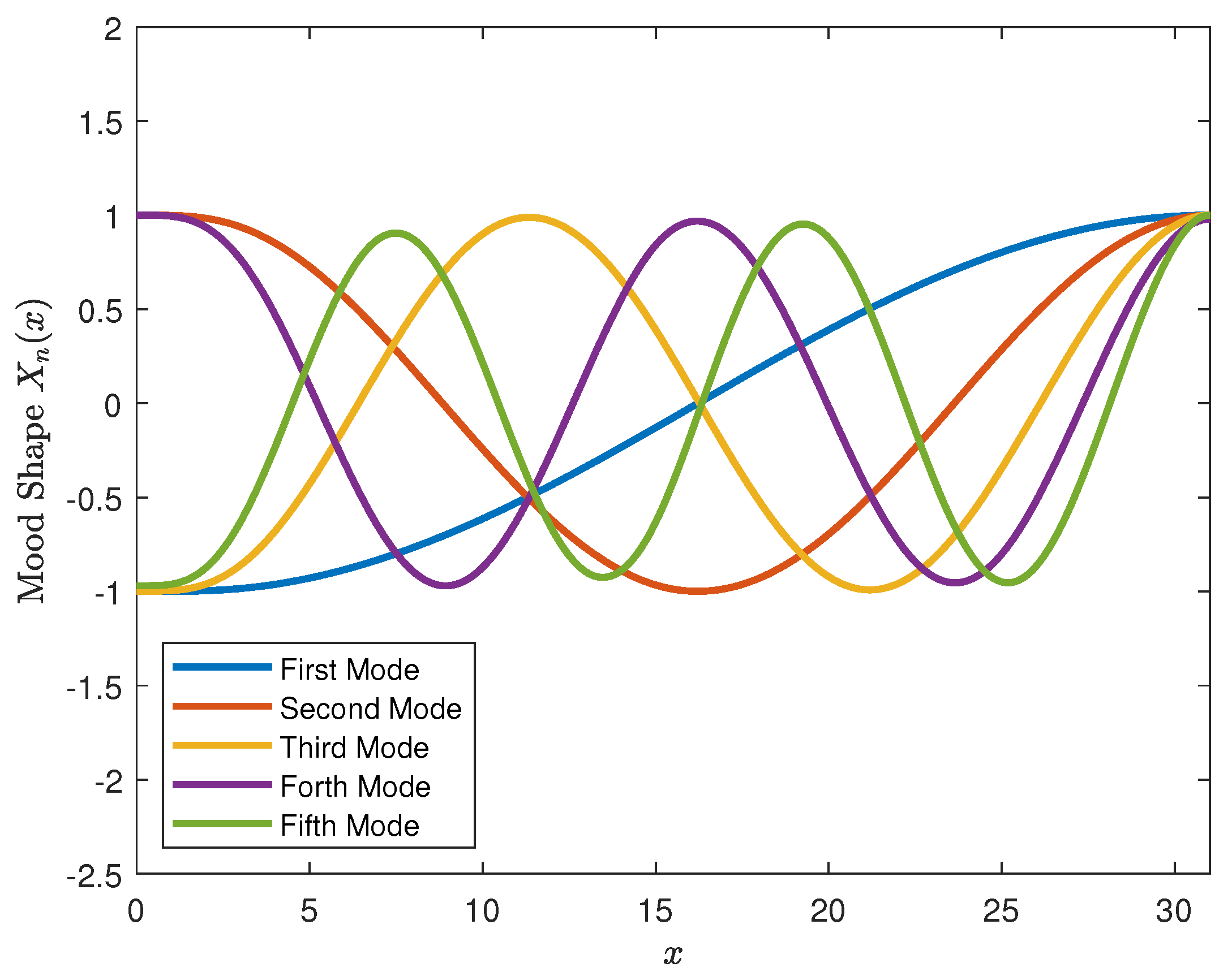
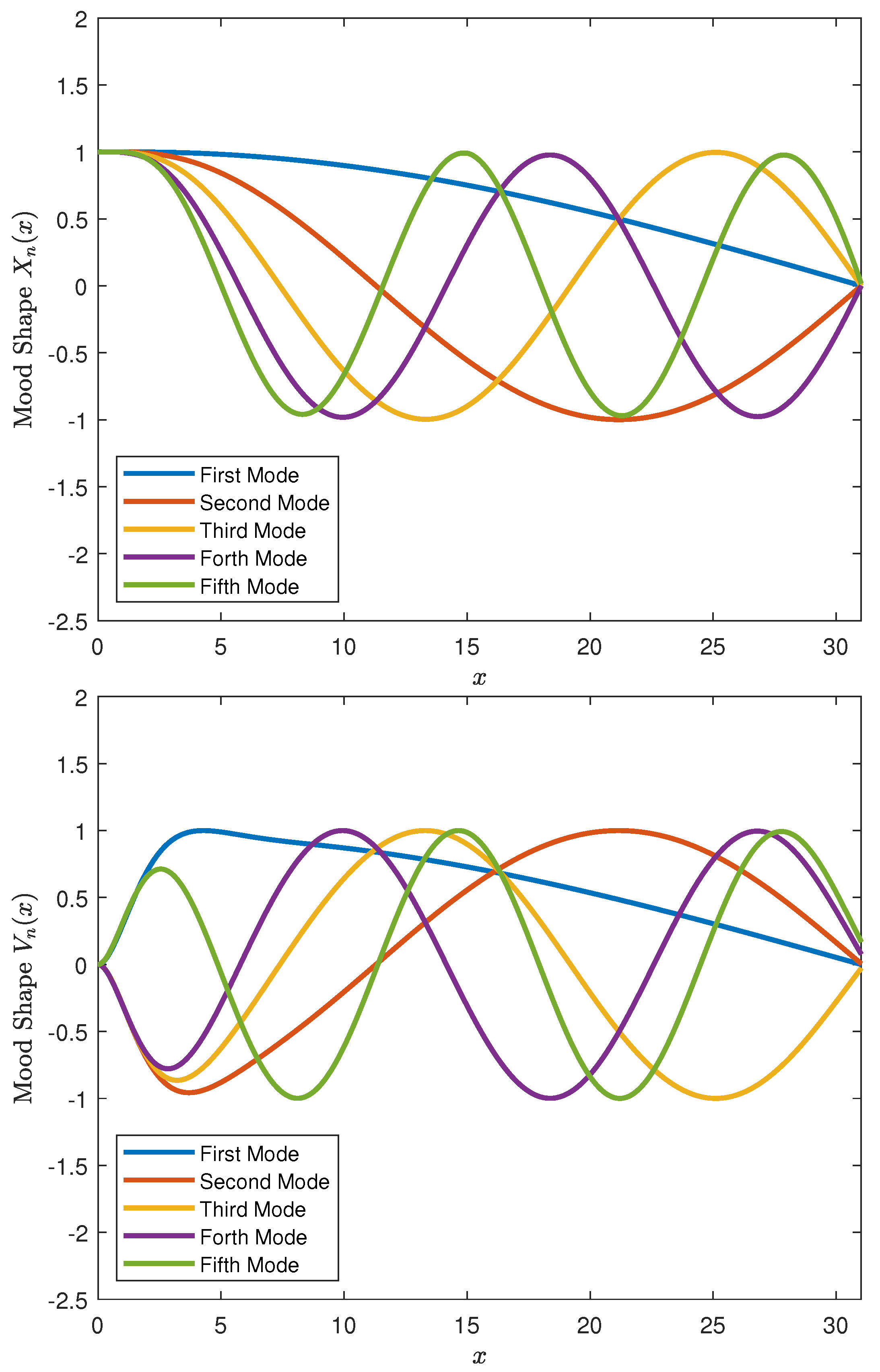
As shown in Figure 3, we set ${\displaystyle \frac{\lambda }{\alpha }}=0$ and obtained the same result as in [19], which was a normal, clamped-free ice shelf without a crack. The value of the crack stiffness ${\displaystyle \frac{\lambda }{\alpha }}$ had a significant impact on the calculation of the mode shape.

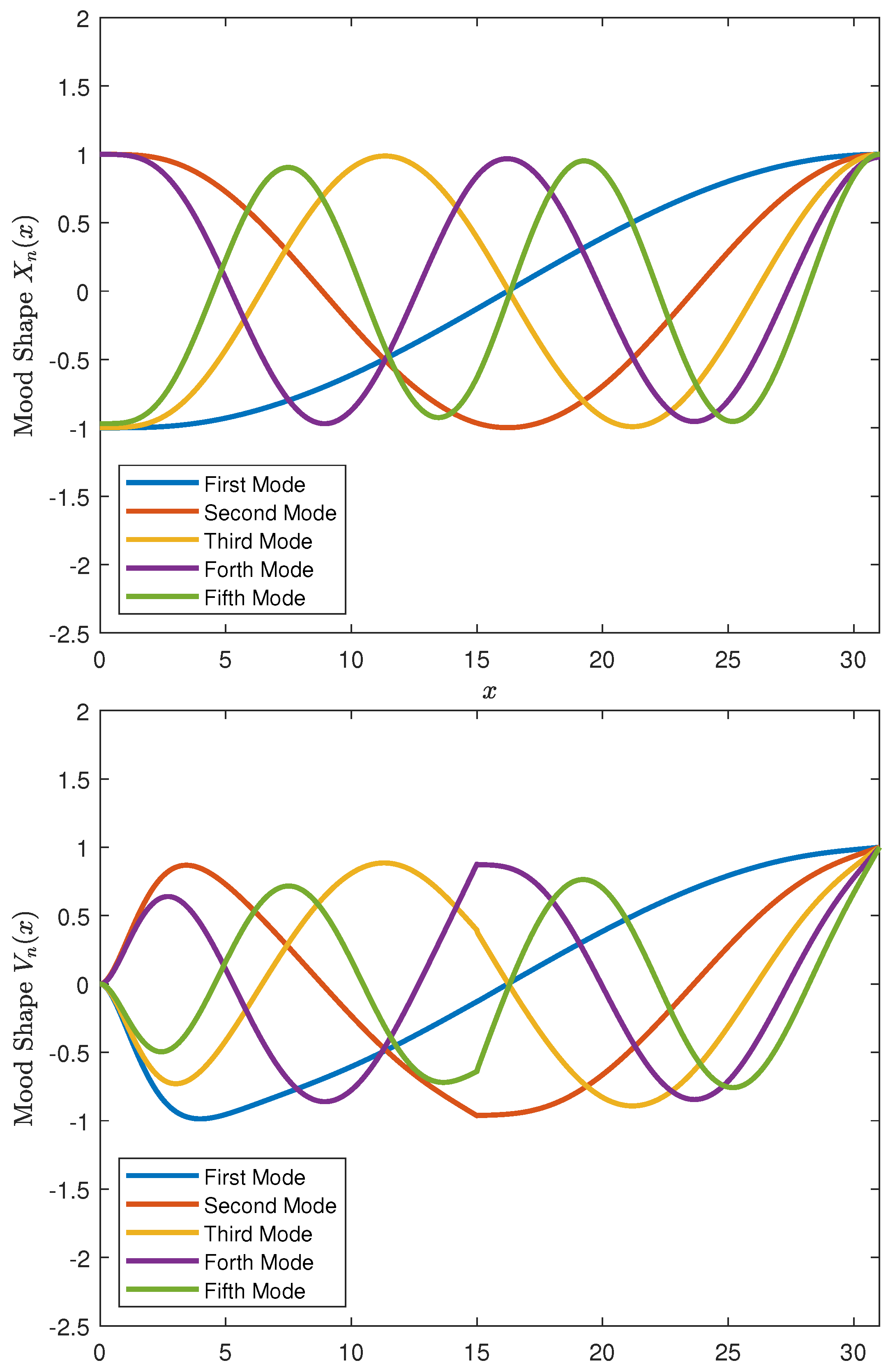
On the other hand, Figure 4 shows the first five mode shapes of the no-flux case for $X_n\left(x\right)$ and $V_n\left(x\right)$ in nondimensional units, where we set the value of the crack stiffness as ${\displaystyle \frac{\lambda }{\alpha }}=112.5607$, which was calculated from the previous formula. In this case, we could clearly see the effect of ${\displaystyle \frac{\lambda }{\alpha }}$ on the mode shape plotting for the vertical displacement $V_n\left(x\right)$.

We next considered the no-pressure condition, which meant that the fluid could flow in and out at the seaward end but the pressure remained constant. The boundary conditions for the clamped end remained the same as in the no-flux condition, but for the free end, we applied the no-pressure condition [30]. Thus, the boundary conditions were as follows:

$$X^{\prime }\left(x^{-}\right)=0,X^{″}\left(x^{-}\right)=0\mathrm{and}{X}^{‴}\left(x^{-}\right)=0\mathrm{at}x=0,$$

(27)

$$X\left(x^{+}\right)=0,X^{\prime \prime \prime \prime }\left(x^{+}\right)=0\mathrm{and}{X}^{\prime \prime \prime \prime \prime }\left(x^{+}\right)=0\mathrm{at}x=L.$$

(28)

At the crack location, the conditions were the same as in the previous case. Imposing the boundary conditions into the mode shape equation yielded a system of twelve linear equations $\mathbf{Ac}=\mathbf{0}$. The matrix was as follows:

$$\left[\begin{array}{cccccccccccc}{k}_1& k_2& k_3& k_4& k_5& k_6& 0& 0& 0& 0& 0& 0\\ k_1^2& k_2^2& k_3^2& k_4^2& k_5^2& k_6^2& 0& 0& 0& 0& 0& 0\\ k_1^3& k_2^3& k_3^3& k_4^3& k_5^3& k_6^3& 0& 0& 0& 0& 0& 0\\ 0& 0& 0& 0& 0& 0& e^{k_{1}L}& e^{k_{2}L}& e^{k_{3}L}& e^{k_{4}L}& e^{k_{5}L}& e^{k_{6}L}\\ 0& 0& 0& 0& 0& 0& k_1^4{e}^{k_{1}L}& k_2^4{e}^{k_{2}L}& k_3^4{e}^{k_{3}L}& k_4^4{e}^{k_{4}L}& k_5^4{e}^{k_{5}L}& k_6^4{e}^{k_{6}L}\\ 0& 0& 0& 0& 0& 0& k_1^5{e}^{k_{1}L}& k_2^5{e}^{k_{2}L}& k_3^5{e}^{k_{3}L}& k_4^5{e}^{k_{4}L}& k_5^5{e}^{k_{5}L}& k_6^5{e}^{k_{6}L}\\ e^{k_{1}S}& e^{k_{2}S}& e^{k_{3}S}& e^{k_{4}S}& e^{k_{5}S}& e^{k_{6}S}& -e^{k_{1}S}& -e^{k_{2}S}& -e^{k_{3}S}& -e^{k_{4}S}& -e^{k_{5}S}& -e^{k_{6}S}\\ k_1{e}^{k_{1}S}& k_2{e}^{k_{2}S}& k_3{e}^{k_{3}S}& k_4{e}^{k_{4}S}& k_5{e}^{k_{5}S}& k_6{e}^{k_{6}S}& -k_1{e}^{k_{1}S}& -k_2{e}^{k_{2}S}& -k_3{e}^{k_{3}S}& -k_4{e}^{k_{4}S}& -k_5{e}^{k_{5}S}& -k_6{e}^{k_{6}S}\\ k_1^2{e}^{k_{1}S}& k_2^2{e}^{k_{2}S}& k_3^2{e}^{k_{3}S}& k_4^2{e}^{k_{4}S}& k_5^2{e}^{k_{5}S}& k_6^2{e}^{k_{6}S}& -k_1^2{e}^{k_{1}S}& -k_2^2{e}^{k_{2}S}& -k_3^2{e}^{k_{3}S}& -k_4^2{e}^{k_{4}S}& -k_5^2{e}^{k_{5}S}& -k_6^2{e}^{k_{6}S}\\ k_1^4{e}^{k_{1}S}& k_2^4{e}^{k_{2}S}& k_3^4{e}^{k_{3}S}& k_4^4{e}^{k_{4}S}& k_5^4{e}^{k_{5}S}& k_6^4{e}^{k_{6}S}& -k_1^4{e}^{k_{1}S}& -k_2^4{e}^{k_{2}S}& -k_3^4{e}^{k_{3}S}& -k_4^4{e}^{k_{4}S}& -k_5^4{e}^{k_{5}S}& -k_6^4{e}^{k_{6}S}\\ k_1^5{e}^{k_{1}S}& k_2^5{e}^{k_{2}S}& k_3^5{e}^{k_{3}S}& k_4^5{e}^{k_{4}S}& k_5^5{e}^{k_{5}S}& k_6^5{e}^{k_{6}S}& -k_1^5{e}^{k_{1}S}& -k_2^5{e}^{k_{2}S}& -k_3^5{e}^{k_{3}S}& -k_4^5{e}^{k_{4}S}& -k_5^5{e}^{k_{5}S}& -k_6^5{e}^{k_{6}S}\\ K_m& K_m& K_m& K_m& K_m& K_m& -k_1^3{e}^{k_{1}S}& -k_2^3{e}^{k_{2}S}& -k_3^3{e}^{k_{3}S}& -k_4^3{e}^{k_{4}S}& -k_5^3{e}^{k_{5}S}& -k_6^3{e}^{k_{6}S}\end{array}\right]\times \left[\begin{array}{c}c1\\ c2\\ c3\\ c4\\ c5\\ c6\\ d1\\ d2\\ d3\\ d4\\ d5\\ d6\end{array}\right]=0.$$

where $K_m=k_m^3{e}^{k_{m}S}+{\displaystyle \frac{\lambda }{\alpha }}{k}_m^4{e}^{k_{m}S}$, ($m=1,...,6)$. Similar to the previous solution, we needed to find the value of $\omega$ that made $\mathrm{A}\left(\omega \right)$ singular; then, we found the coefficients $c_n$ and $d_n$ from the corresponding zero eigenvector. We also needed to stabilise the matrix with the same method we used before by multiplying the vectors $c_n$ and $d_n$ by an exponential function. The final result was in the following form:

$$\left[\begin{array}{cccccccccccc}{k}_1{e}^{-k_{1}S}& k_2{e}^{-k_{2}S}& k_3{e}^{-k_{3}S}& k_4& k_5& k_6& 0& 0& 0& 0& 0& 0\\ k_1^2{e}^{-k_{1}S}& k_2^2{e}^{-k_{2}S}& k_3^2{e}^{-k_{3}S}& k_4^2& k_5^2& k_6^2& 0& 0& 0& 0& 0& 0\\ k_1^3{e}^{-k_{1}S}& k_2^3{e}^{-k_{2}S}& k_3^3{e}^{-k_{3}S}& k_4^3& k_5^3& k_6^3& 0& 0& 0& 0& 0& 0\\ 0& 0& 0& 0& 0& 0& 1& 1& 1& e^{k_4(L-S)}& e^{k_5(L-S)}& e^{k_6(L-S)}\\ 0& 0& 0& 0& 0& 0& k_1^4& k_2^4& k_3^4& k_4^4{e}^{k_4(L-S)}& k_5^4{e}^{k_5(L-S)}& k_6^4{e}^{k_6(L-S)}\\ 0& 0& 0& 0& 0& 0& k_1^5& k_2^5& k_3^5& k_4^5{e}^{k_4(L-S)}& k_5^5{e}^{k_5(L-S)}& k_6^5{e}^{k_6(L-S)}\\ 1& 1& 1& e^{k_{4}S}& e^{k_{5}S}& e^{k_{6}S}& -e^{k_1(S-L)}& -e^{k_2(S-L)}& -e^{k_3(S-L)}& -1& -1& -1\\ k_1& k_2& k_3& k_4{e}^{k_{4}S}& k_5{e}^{k_{5}S}& k_6{e}^{k_{6}S}& -k_1{e}^{k_1(S-L)}& -k_2{e}^{k_2(S-L)}& -k_3{e}^{k_3(S-L)}& -k_4& -k_5& -k_6\\ k_1^2& k_2^2& k_3^2& k_4^2{e}^{k_{4}S}& k_5^2{e}^{k_{5}S}& k_6^2{e}^{k_{6}S}& -k_1^2{e}^{k_1(S-L)}& -k_2^2{e}^{k_2(S-L)}& -k_3^2{e}^{k_3(S-L)}& -k_4^2& -k_5^2& -k_6^2\\ k_1^4& k_2^4& k_3^4& k_4^4{e}^{k_{4}S}& k_5^4{e}^{k_{5}S}& k_6^4{e}^{k_{6}S}& -k_1^4{e}^{k_1(S-L)}& -k_2^4{e}^{k_2(S-L)}& -k_3^4{e}^{k_3(S-L)}& -k_4^4& -k_5^4& -k_6^4\\ k_1^5& k_2^5& k_3^5& k_4^5{e}^{k_{4}S}& k_5^5{e}^{k_{5}S}& k_6^5{e}^{k_{6}S}& -k_1^5{e}^{k_1(S-L)}& -k_2^5{e}^{k_2(S-L)}& -k_3^5{e}^{k_3(S-L)}& -k_4^5& -k_5^5& -k_6^5\\ K_1^2+{\displaystyle \frac{\lambda }{\alpha }}{k}_1^4& K_2^2+{\displaystyle \frac{\lambda }{\alpha }}{k}_2^4& K_3^2+{\displaystyle \frac{\lambda }{\alpha }}{k}_3^4& K_m& K_m& K_m& -k_1^3{e}^{k_1(S-L)}& -k_2^3{e}^{k_2(S-L)}& -k_3^3{e}^{k_3(S-L)}& -k_4^3& -k_5^3& -k_6^3\end{array}\right]$$

$$\times \left[\begin{array}{c}\widehat{c}1\\ \widehat{c}2\\ \widehat{c}3\\ \widehat{c}4\\ \widehat{c}5\\ \widehat{c}6\\ \widehat{d}1\\ \widehat{d}2\\ \widehat{d}3\\ \widehat{d}4\\ \widehat{d}5\\ \widehat{d}6\end{array}\right]=0.$$

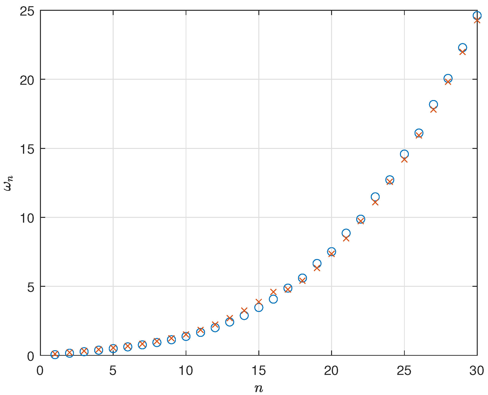
By comparing the two

Table 1. Non-dimensional angular frequencies ${\omega }_n$ and dimensional periods $T_n$ of modes for the no-flux case, where the dimensional length of the cracked ice shelf $L=40$ km when $M=0.0162$ and $M=0$.

	$\mathit{M}=0.0162$		$\mathit{M}=0$
n	${\omega }_n$	$T_n$	${\omega }_n$	$T_n$
1	0.10613	0.67701 h	0.10614	0.67695 h
2	0.21253	0.33808 h	0.21261	0.33796 h
3	0.32014	0.22445 h	0.32039	0.22427 h
4	0.43116	0.16665 h	0.43178	0.16641 h
5	0.54961	0.13073 h	0.55082	0.13045 h
10	1.51175	171.113 s	1.52461	169.669 s
15	3.87393	66.7747 s	3.94702	65.5383 s
20	7.35072	35.1913 s	8.76451	29.5146 s
25	14.1932	18.2256 s	16.7541	15.4398 s
30	24.2845	10.6521 s	28.6811	9.01921 s

and

Table 2. Non-dimensional angular frequencies ${\omega }_n$ and dimensional periods $T_n$ of modes for the no-pressure case, where the dimensional length of the cracked ice shelf $L=40$ km when $M=0.0162$ and $M=0$.

	$\mathit{M}=0.0162$		$\mathit{M}=0$
n	${\omega }_n$	$T_n$	${\omega }_n$	$T_n$
1	0.05306	1.35422 h	0.05306	1.35419 h
2	0.15930	0.45107 h	0.15933	0.45098 h
3	0.26626	0.26986 h	0.26641	0.26971 h
4	0.37566	0.19127 h	0.37607	0.19106 h
5	0.49087	0.14638 h	0.49176	0.14611 h
10	1.37497	188.139 s	1.38673	186.539 s
15	3.47097	74.5270 s	3.54124	73.0482 s
20	7.51409	34.4261 s	6.86932	37.6574 s
25	14.5845	17.7366 s	13.3130	19.4306 s
30	24.6155	10.5088 s	23.9252	10.8120 s

, we can see that the dimensional periods $T_n$ were higher for the no-pressure case compared to the no-flux case. Now, comparing our solution with the results in [14,19], we can clearly see that the time periods were significantly lower for both the no-flux and no-pressure cases than in our results. In Figure 5 and Figure 6, we can see a comparison with our two cases for 30 periods.

The plots of the mode shapes for the potential velocity and vertical displacement are shown in Figure 7 and Figure 8. The crack stiffnesses were set to ${\displaystyle \frac{\lambda }{\alpha }}=0$ and ${\displaystyle \frac{\lambda }{\alpha }}=21.6331$, respectively.

3. Simulating Cracked Ice Shelf Vibrations

To simulate the vibration of the ice shelf in the time domain, we used the general solution formula in terms of modes for both the potential $\Phi (x,t)$ and the vertical displacement $\eta (x,t)$ as follows:

$$\Phi (x,t)=\sum _{n=0\mathrm{or}1}^{\infty }{A}_n{X}_n\left(x\right)cos\left({\omega }_{n}t\right)+\sum _{n=1}^{\infty }{\displaystyle \frac{B_n}{{\omega }_n}}{X}_n\left(x\right)sin\left({\omega }_{n}t\right),$$

(29)

$$\eta (x,t)=\sum _{n=1}^{\infty }{G}_n{V}_n\left(x\right)cos\left({\omega }_{n}t\right)+\sum _{n=1}^{\infty }{\displaystyle \frac{S_n}{{\omega }_n}}{V}_n\left(x\right)sin\left({\omega }_{n}t\right),$$

(30)

where $A_n$ is found from the initial value of $\Phi$, $B_n$ is found from the initial time derivative of $\Phi$, $G_n$ is found from the initial position at $t=0$, and $S_n$ is found from the initial velocity.

The sum began at one for all cases except for the no-flux case in the potential $\Phi$; the sum of the first term started at zero. This is the same as that found in [19] for an ice shelf without a crack.

We solved Equation (29) to determine the constant $A_n$ along with the initial conditions $\Phi (x,0)=f\left(x\right)$ and ${\Phi }_t(x,0)=0$. This led to

$$\sum _{n=0}^{\infty }{A}_n{X}_n=f\left(x\right)$$

(31)

We solved this by multiplying Equation (31) by ${\mathrm{X}}_{\mathrm{m}}$ and integrating them to obtain

$${\int }_0^{L}f\left(x\right)X_{m}dx=\sum _{n=0}^{\infty }{A}_n{\int }_0^L{X}_n{X}_{m}dx.$$

(32)

In order to find the solution for the integral component, since we knew that the mode shapes ${\mathrm{X}}_{\mathrm{n}}$ were not orthogonal with respect to the inner product, we used numerical quadrature. The integral approximation was in the following form:

$$\sum _{i=1}^{N}f\left(x_i\right)X_m\left(x_i\right)w_i=\sum _{n=0}^{\infty }{A}_n\sum _{i=1}^N{X}_n\left(x_i\right)X_m\left(x_i\right)w_i,$$

(33)

Here, N is the number of data points or nodes used in the approximation, $w_i$ are the weights associated with each data point, and $x_i$ are the positions of the data points within the interval $[0,L]$.

In this case, we used the numerical integration to convert an integral into matrix multiplication. We then had the approximation for the definite integral as the following matrix:

$$\mathrm{X}=\left[X_m\left(x_n\right)\right]$$

and vectors $\mathrm{f}=\left[f\left(x_n\right)\right],\mathrm{w}=\left[w_n\right]$, and $\mathrm{A}=\left[A_n\right]$. Equation (33) became

$$\mathrm{X}\mathrm{diag}\left(\mathrm{w}\right){\mathrm{X}}^{\mathrm{T}}\mathrm{A}=\mathrm{X}\mathrm{diag}\left(\mathrm{w}\right)\mathrm{f},$$

This led to

$$\mathrm{A}={\displaystyle \frac{\mathrm{X}\mathrm{diag}\left(\mathrm{w}\right)\mathrm{f}}{\mathrm{X}\mathrm{diag}\left(\mathrm{w}\right){\mathrm{X}}^{\mathrm{T}}}}.$$

where $\mathrm{diag}$ means the diagonal matrix with the vector elements on the diagonal and the superscript $\mathrm{T}$ is the matrix transpose.

Now, we could write the solution for the potential equation in 29 in matrix multiplication form as

$$\Phi (x,t)={\mathrm{X}}^{\mathrm{T}}\mathrm{diag}[cos\left({\omega }_{n}t\right)]\mathrm{A}.$$

By this efficient method, we could now calculate the time-dependent motion. For the solution of a non-zero initial time derivative for both the potential and the displacement, we used the same calculation methods.

4. Results

Here, we present simulations of the motion of a cracked ice shelf in the time domain. As in [19], we started by simulating the potential velocity $\Phi$.

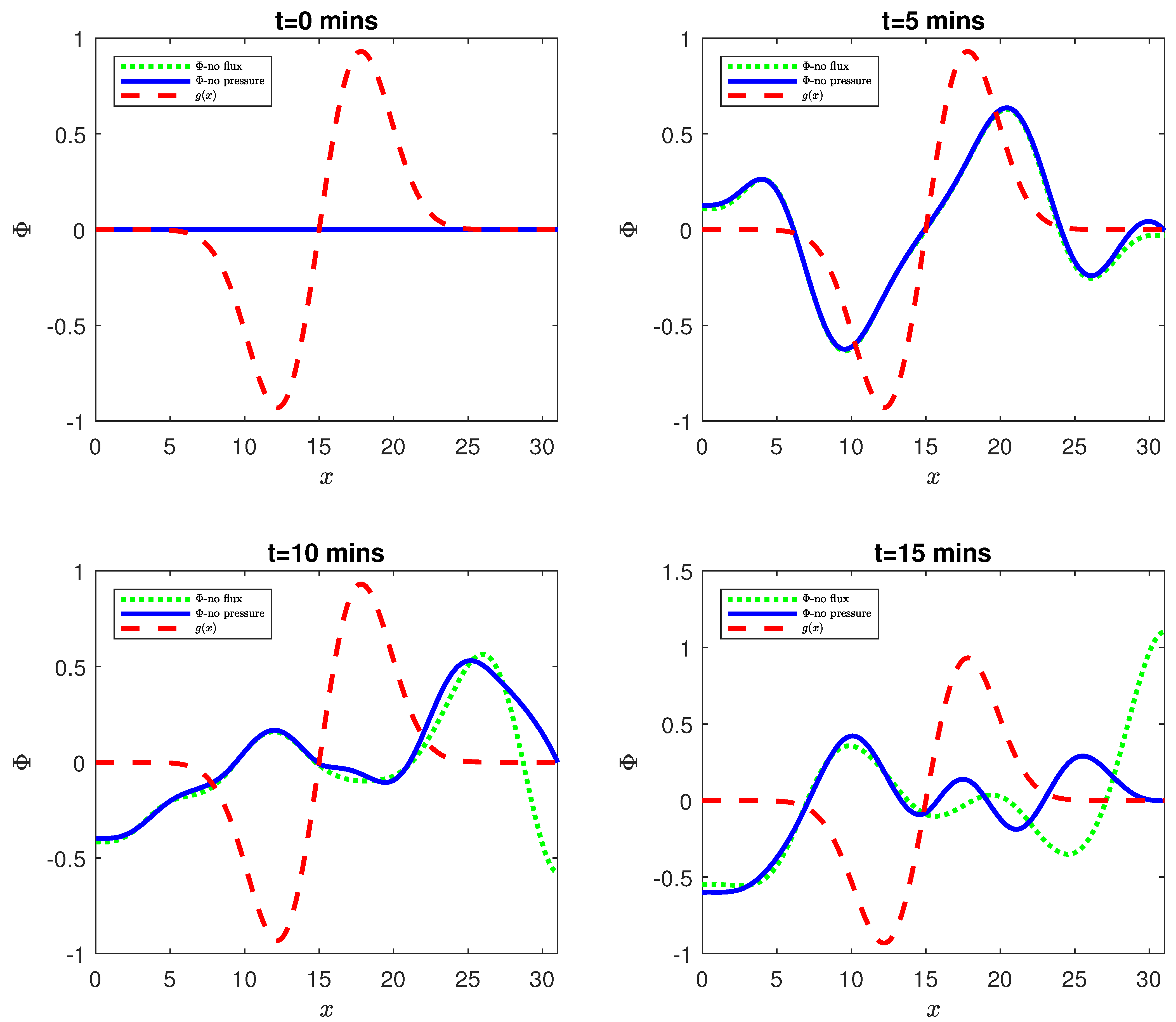
By applying the initial conditions $\Phi (x,0)=f\left(x\right)$ and ${\Phi }_t(x,0)=0$ to Equation (29), we simulated the solution as shown in Figure 9.

Here, we used the same Gaussian functions in the simulations as in [19] to see what would happen if we applied our cracked conditions to the ice shelf. In the first simulation, we could see the cases of no flux (green) and no pressure (blue), and the initial function $f\left(x\right)$ (red). Here, the Gaussian function was

$$f\left(x\right)=\exp (-{(x-5)}^2/10).$$

(34)

The simulation for the Equation (29) solution applying the initial conditions $\Phi (x,0)=0$ and ${\Phi }_t(x,0)=g\left(x\right)$ is shown in Figure 10, where

$$g\left(x\right)=exp(-{(x-17.5)}^2/10)-exp(-{(x-12.5)}^2/10).$$

(35)

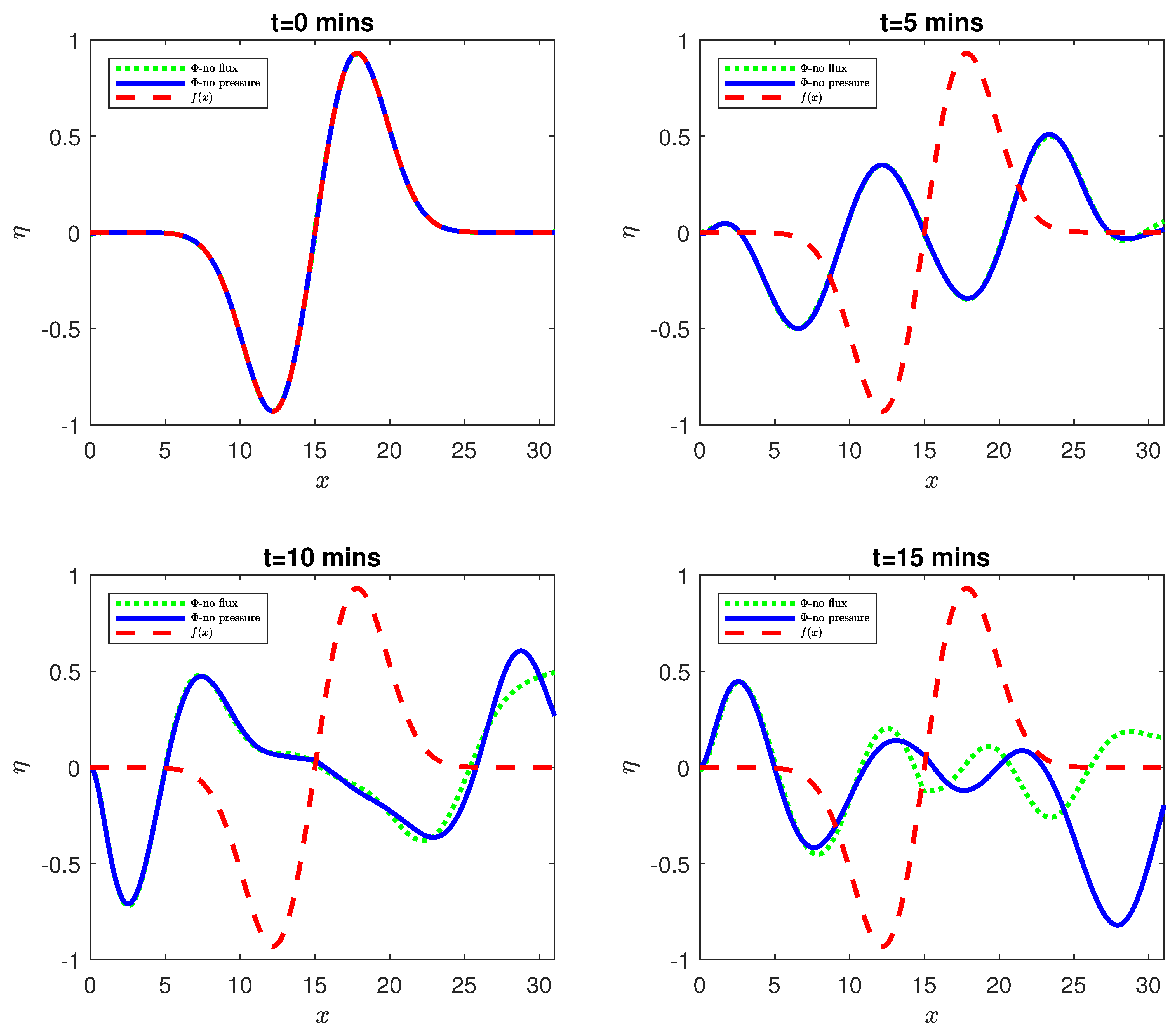
For the vertical displacement $\eta$, we applied the initial conditions $\eta (x,0)=f\left(x\right)$ and ${\eta }_t(x,0)=0$ to Equation (30). The solution for the case of no flux (green), the case of no pressure (blue), and the Gaussian function $f\left(x\right)$ (red) are shown in Figure 11, where

$$f\left(x\right)=exp(-{(x-17.5)}^2/10)-exp(-{(x-12.5)}^2/10).$$

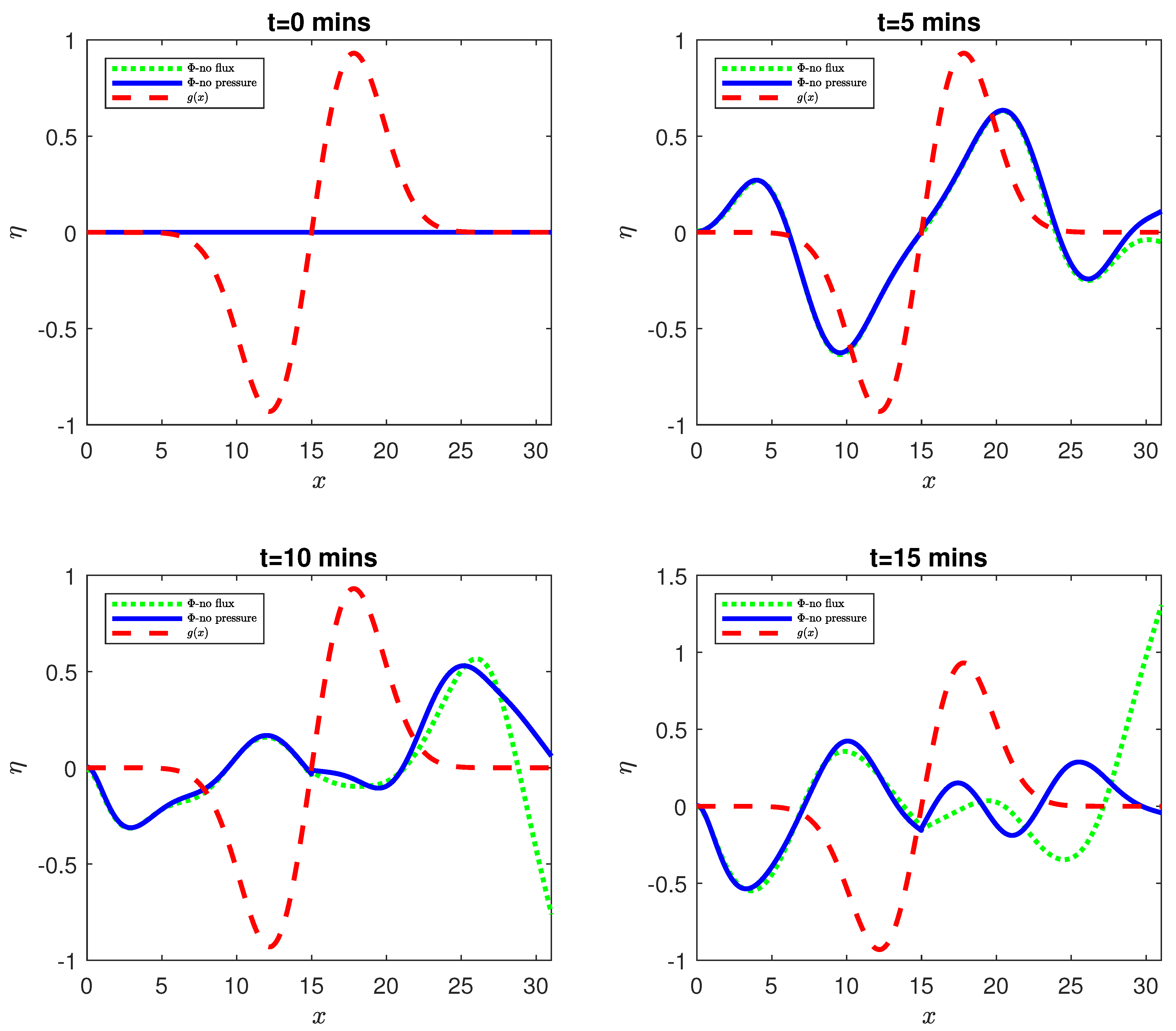
In Figure 12, we present the solution for the vertical displacement if we applied the initial conditions $\eta (x,0)=0$ and ${\eta }_t(x,0)=g\left(x\right)$, where

$$g\left(x\right)=exp(-{(x-17.5)}^2/10)-exp(-{(x-12.5)}^2/10).$$

From the two Figure 11 and Figure 12 of the vertical displacement, we can see that it matched the boundary conditions as a clamped-free cracked ice shelf, with the crack acting as rotational spring at $x=15$.

5. Discussion: Application to Ice Shelf Breakup

This work is the first step in the attempt to model the growth of cracks in ice shelves due to flexural vibration. It is important to note that there are many mechanisms that could cause ice shelf break up and that flexural vibration is only one possible mechanism. Previous studies of fracture include [33], which considered a narrow bridge of floating ice that connected the Wilkins Ice Shelf, Antarctica, to two confining islands that eventually collapsed, and postulated that both cyclic and monotonic components of motion contributed. Ref. [34] modelled rifts in the Larsen B Ice Shelf and showed that most of the rift extension occurred in bursts after overcoming the resistance of suture zones that bound neighbouring glacier inflows. Ref. [35] studied a rift in the Brunt Ice Shelf, East Antarctica, and found alternating episodes of fast and slow propagation of the rift tip, controlled by the heterogeneous structure of the ice shelf. Ref. [36] studied the Larsen C Ice Shelf and found that thinning of the ice mélange was sufficient to reactivate the rifts and trigger a major calving.

It is important to note that our current model is two-dimensional and we could not simulate the growth of rifts; moreover, as mentioned, there is not conclusive evidence that vibration is critical to this process. However, it seems to be a likely cause and requires investigation and modelling. The key result here is to show how we can model the time-domain motion of an ice shelf (rather than the frequency domain). The growth of cracks occur in the time domain, so such simulations are essential. The next stage is to consider the growth of cracks and simulate ice shelf breakup in two dimensions and then extend to three dimensions.

6. Conclusions

This study presents a framework for modelling the vibrations of cracked ice shelves, using the Euler–Bernoulli beam theory and shallow water approximation to account for the interaction between the ice shelf and the underlying ocean, with a cracked beam theory developed separately. This models the cracks as rotational springs and captures the impact of stiffness discontinuities on vibration patterns, natural frequencies, and mode shapes.

The results show that crack stiffness significantly alters the dynamic behaviour of ice shelves. Higher stiffness leads to increased natural frequencies and localised vibrations, while lower stiffness results in greater vertical displacement, highlighting areas of potential instability. The no-flux and no-pressure boundary conditions provided different scenarios for analysing the ice shelf response.

This work is an extension of the time domain modelling of [19] to include the effect of a crack. The work is preliminary and the model is greatly simplified. Although model simplifications limit this study, the next step in this model is to include the time-dependent growth of a crack caused by ice shelf flexure. There are many ways in which this study could be extended; for example, the effect of incident waves could be considered following [37]. The effects of variations in depth or ice shelf thickness could easily be incorporated into the current model paradigm. More complex extensions could include three-dimensional modelling, dynamic crack growth, and the integration of environmental factors such as temperature variations, ocean currents, and wind forces. This work is a first step towards modelling crack growth so that we can analyse and anticipate ice shelf collapse.

References

1. DeConto, R.M.; Pollard, D. Contribution of Antarctica to past and future sea-level rise. Nature 2016, 531, 591–597. [Google Scholar] [CrossRef]
2. Rignot, E.; Jacobs, S.; Mouginot, J.; Scheuchl, B. Ice-shelf melting around Antarctica. Science 2013, 341, 266–270. [Google Scholar] [CrossRef]
3. Snow, N.; Center, I.D. Why Ice Shelves Matter. National Snow and Ice Data Center a Part of CIRES at the University of Colorado Boulder. Available online: https://nsidc.org/learn/parts-cryosphere/ice-shelves/why-ice-shelves-matter#:~:text=on%20ice%20shelves-,Why%20they%20matter,are%20already%20floating%20on%20water (accessed on 24 January 2023).
4. NASA Earth Observatory. Breakup at Brunt. NASA Earth Observatory. 2021. Available online: https://earthobservatory.nasa.gov/images/150880/antarcticas-brunt-ice-shelf-finally-breaks (accessed on 24 January 2023).
5. British Antarctic Survey. Brunt Ice Shelf in Antarctica Calves Giant Iceberg; British Antarctic Survey: Cambridge, UK, 2023. [Google Scholar]
6. U.S. National Ice Center Latest News. Brunt Ice Shelf; U.S. National Ice Center Latest News: Suitland, MD, USA, 2023.
7. Sun, S.; Cornford, S.L.; Liu, Y.; Moore, J.C. Dynamic response of Antarctic ice shelves to bedrock uncertainty. Cryosphere 2014, 8, 1561–1576. [Google Scholar] [CrossRef]
8. Brunt, K.M.; Okal, E.A.; MacAyeal, D.R. Antarctic ice-shelf calving triggered by the Honshu (Japan) earthquake and tsunami, March 2011. J. Glaciol. 2011, 57, 785–788. [Google Scholar] [CrossRef]
9. Massom, R.A.; Scambos, T.A.; Bennetts, L.G.; Reid, P.; Squire, V.A.; Stammerjohn, S.E. Antarctic ice shelf disintegration triggered by sea ice loss and ocean swell. Nature 2018, 558, 383–389. [Google Scholar] [CrossRef] [PubMed]
10. Bromirski, P.D.; Chen, Z.; Stephen, R.A.; Gerstoft, P.; Arcas, D.; Diez, A.; Aster, R.C.; Wiens, D.A.; Nyblade, A. Tsunami and infragravity waves impacting A ntarctic ice shelves. J. Geophys. Res. Ocean. 2017, 122, 5786–5801. [Google Scholar]
11. Liang, J.; Pitt, J.P.; Bennetts, L.G. Pan-Antarctic assessment of ice shelf flexural responses to ocean waves. J. Geophys. Res. Ocean. 2024, 129, e2023JC020824. [Google Scholar]
12. Holdsworth, G.; Glynn, J. Iceberg calving from floating glaciers by a vibrating mechanism. Nature 1978, 274, 464–466. [Google Scholar] [CrossRef]
13. Reeh, N. On the calving of ice from floating glaciers and ice shelves. J. Glaciol. 1968, 7, 215–232. [Google Scholar] [CrossRef]
14. Meylan, M.H.; Bennetts, L.G.; Hosking, R.J.; Catt, E. On the calculation of normal modes of a coupled ice-shelf/sub-ice-shelf cavity system. J. Glaciol. 2017, 63, 751–754. [Google Scholar] [CrossRef]
15. Sergienko, O.V. Normal modes of a coupled ice-shelf/sub-ice-shelf cavity system. J. Glaciol. 2013, 59, 76–80. [Google Scholar] [CrossRef]
16. Kalyanaraman, B.; Meylan, M.H.; Bennetts, L.G.; Lamichhane, B.P. A coupled fluid-elasticity model for the wave forcing of an ice-shelf. J. Fluids Struct. 2020, 97, 103074. [Google Scholar] [CrossRef]
17. Papathanasiou, T.; Karperaki, A.; Theotokoglou, E.; Belibassakis, K. A higher order FEM for time-domain hydroelastic analysis of large floating bodies in an inhomogeneous shallow water environment. Proc. R. Soc. A Math. Phys. Eng. Sci. 2015, 471, 20140643. [Google Scholar] [CrossRef]
18. Bennetts, L.G.; Meylan, M.H. Complex resonant ice shelf vibrations. SIAM J. Appl. Math. 2021, 81, 1483–1502. [Google Scholar] [CrossRef]
19. Aljabri, R.; Meylan, M.H. Time Domain Vibration Analysis of an Ice Shelf. J. Mar. Sci. Eng. 2024, 12, 468. [Google Scholar] [CrossRef]
20. Alshahrani, F.; Meylan, M.H.; Wilks, B. Transient Shallow Water Wave Interactions with a Partially Fragmented Ice Shelf. Fluids 2024, 9, 192. [Google Scholar] [CrossRef]
21. Bennetts, L.G.; Williams, T.D.; Porter, R. A thin-plate approximation for ocean wave interactions with an ice shelf. J. Fluid Mech. 2024, 984, A48. [Google Scholar]
22. Chondros, T.; Dimarogonas, A.; Yao, J. A continuous cracked beam vibration theory. J. Sound Vib. 1998, 215, 17–34. [Google Scholar] [CrossRef]
23. Mungla, M.J.; Sharma, D.; Makwana, H.; Bhavsar, R. Inverse dynamics of cracked cantilever beam. In Proceedings of the International Conference in Advanced Design and Manufacturing, Montreal, QC, Canada, 13–15 August 2014; pp. 331–336. [Google Scholar]
24. Mungla, M.J.; Sharma, D.S.; Trivedi, R.R. Identification of a crack in clamped-clamped beam using frequency-based method and genetic algorithm. Procedia Eng. 2016, 144, 1426–1434. [Google Scholar] [CrossRef]
25. Chati, M.; Rand, R.; Mukherjee, S. Modal analysis of a cracked beam. J. Sound Vib. 1997, 207, 249–270. [Google Scholar] [CrossRef]
26. Saavedra, P.; Cuitino, L. Crack detection and vibration behavior of cracked beams. Comput. Struct. 2001, 79, 1451–1459. [Google Scholar] [CrossRef]
27. Nguyen, K.V. Mode shapes analysis of a cracked beam and its application for crack detection. J. Sound Vib. 2014, 333, 848–872. [Google Scholar] [CrossRef]
28. Chang, C.C.; Chen, L.W. Detection of the location and size of cracks in the multiple cracked beam by spatial wavelet based approach. Mech. Syst. Signal Process. 2005, 19, 139–155. [Google Scholar] [CrossRef]
29. Dimarogonas, A.D.; Paipetis, S.A.; Chondros, T.G. Analytical Methods in Rotor Dynamics; Springer Science & Business Media: Berlin, Germany, 2013. [Google Scholar]
30. Papathanasiou, T.K.; Karperaki, A.E.; Belibassakis, K.A. On the resonant hydroelastic behaviour of ice shelves. Ocean Model. 2019, 133, 11–26. [Google Scholar] [CrossRef]
31. Stoker, J.J. Water Waves: The Mathematical Theory with Applications; John Wiley & Sons: Hoboken, NJ, USA, 1992; Volume 36. [Google Scholar]
32. Fox, C. A scaling law for the flexural motion of floating ice. In Proceedings of the IUTAM Symposium on Scaling Laws in Ice Mechanics and Ice Dynamics: Proceedings of the IUTAM Symposium, Fairbanks, AK, USA, 13–16 June 2000; Springer: Berlin/Heidelberg, Germany, 2001; pp. 135–148. [Google Scholar] [CrossRef]
33. Humbert, A.; Gross, D.; Müller, R.; Braun, M.; Van De Wal, R.; Van Den Broeke, M.; Vaughan, D.; Van De Berg, W. Deformation and failure of the ice bridge on the Wilkins Ice Shelf, Antarctica. Ann. Glaciol. 2010, 51, 49–55. [Google Scholar] [CrossRef]
34. Borstad, C.; McGrath, D.; Pope, A. Fracture propagation and stability of ice shelves governed by ice shelf heterogeneity. Geophys. Res. Lett. 2017, 44, 4186–4194. [Google Scholar] [CrossRef]
35. De Rydt, J.; Gudmundsson, G.H.; Nagler, T.; Wuite, J.; King, E.C. Recent rift formation and impact on the structural integrity of the Brunt Ice Shelf, East Antarctica. Cryosphere 2018, 12, 505–520. [Google Scholar] [CrossRef]
36. Larour, E.; Rignot, E.; Poinelli, M.; Scheuchl, B. Physical processes controlling the rifting of Larsen C Ice Shelf, Antarctica, prior to the calving of iceberg A68. Proc. Natl. Acad. Sci. USA 2021, 118, e2105080118. [Google Scholar] [CrossRef]
37. McNeil, S.; Meylan, M.H. Time-Dependent Modelling of the Wave-Induced Vibration of Ice Shelves. J. Mar. Sci. Eng. 2023, 11, 1191. [Google Scholar] [CrossRef]
Figure 1. Schematic diagram of the ice shelf with one crack.
Glacies 02 00005 g001
Figure 2. Schematic diagram of the cracked ice shelf with spring stiffness α r .
Glacies 02 00005 g002
Figure 3. The first five mode shapes. The top panel is the potential velocity and the bottom panel is the vertical displacement. The crack stiffness λ α = 0 , the ice shelf length L = 40 km, the ice thickness h = 300 m, and the cavity depth H = 100 m. In our nondimensional units, M = 0.0162 and L ¯ = 31.0199 . Note that the x scale is in nondimensional units.
Glacies 02 00005 g003aGlacies 02 00005 g003b
Figure 4. As in Figure except that the crack stiffness λ α = 112.5607 .
Glacies 02 00005 g004
Figure 5. The time periods T h of the modes in hours, comparing the results for the no-flux condition (x) and the no-pressure condition (o). The length of the cracked ice shelf L = 40 km, the ice thickness h = 300 m, the cavity depth H = 100 m, and M = 0.0162 .
Glacies 02 00005 g005
Figure 6. Plot for the 30 nondimensional angular frequencies, ω n , comparing the results for the no-flux condition (x) and the no-pressure condition (o), where the length of the cracked ice shelf L = 40 km, the thickness of the ice h = 300 m, the depth of the cavity H = 100 m, and M = 0.0162 .
Glacies 02 00005 g006
Figure 7. The plots for the no-pressure case with the same values as in Figure 3.
Glacies 02 00005 g007
Figure 8. The plots for the no-pressure case with the same values as in Figure 3 except that the crack stiffness λ α = 21.6331 .
Glacies 02 00005 g008
Figure 9. Simulation of the potential velocity Φ ( x , t ) . The initial conditions ϕ ( x , 0 ) = f ( x ) and Φ t ( x , 0 ) = 0 were given by Equation (34) for the cases of no flux (green) and no pressure (blue) and the initial function f ( x ) (red) for the ice length of L = 40 k; the mode number was N = 50 . The thickness of the ice h = 300 m, the depth of the cavity H = 100 m, and M = 0.9162 . the full solution is provided in the Supplementry Material, Movie S1.
Glacies 02 00005 g009
Figure 10. Simulation for the potential velocity Φ ( x , t ) . The initial conditions ϕ ( x , 0 ) = g ( x ) and Φ t ( x , 0 ) = 0 were given by Equation (35) for the cases of no flux (green) and no pressure (blue) and the initial function g ( x ) (red) for the ice length of L = 40 k; the mode number was N = 50 . The thickness of the ice h = 300 m, the depth of the cavity H = 100 m, and M = 0.9162 . The full solution is provided in the Supplementry Material, Movie S2.
Glacies 02 00005 g010
Figure 11. Simulation for the vertical displacement η ( x , t ) . The initial conditions η ( x , 0 ) = f ( x ) and η t ( x , 0 ) = 0 were given by Equation (34) for the cases of no flux (green) and no pressure (blue) and the initial function f ( x ) (red) for the ice length of L = 40 k; the mode number was N = 50 . The thickness of the ice h = 300 m, the depth of the cavity H = 100 m, and M = 0.9162 . The full solution is provided in the Supplementry Material, Movie S3.
Glacies 02 00005 g011
Figure 12. Simulation for the vertical displacement η ( x , t ) . The initial conditions η ( x , 0 ) = g ( x ) and η t ( x , 0 ) = 0 were given by Equation (34) for the cases of no flux (green) and no pressure (blue) and the initial function g ( x ) (red) for the ice length of L = 40 k; the mode number was N = 50 . The thickness of the ice h = 300 m, the depth of the cavity H = 100 m, and M = 0.9162 . The full solution is provided in the Supplementry Material, Movie S4.
Glacies 02 00005 g012