Configuration and Registration of Multi-Camera Spectral Image Database of Icon Paintings


School of Computing, University of Eastern Finland, P.O. Box 111, FI-80101 Joensuu, Finland
Computation 2019, 7(3), 47; https://doi.org/10.3390/computation7030047
Submission received: 30 June 2019
/
Revised: 19 August 2019
/
Accepted: 27 August 2019
/
Published: 29 August 2019
(This article belongs to the Special Issue Applications of Computation in Multispectral and Hyperspectral Imaging Systems)
Abstract
:At the cost of added complexity and time, hyperspectral imaging provides a more accurate measure of the scene’s irradiance compared to an RGB camera. Several camera designs with more than three channels have been proposed to improve the accuracy. The accuracy is often evaluated based on the estimation quality of the spectral data. Currently, such evaluations are carried out with either simulated data or color charts to relax the spatial registration requirement between the images. To overcome this limitation, this article presents an accurately registered image database of six icon paintings captured with five cameras with different number of channels, ranging from three (RGB) to more than a hundred (hyperspectral camera). Icons are challenging topics because they have complex surfaces that reflect light specularly with a high dynamic range. Two contributions are proposed to tackle this challenge. First, an imaging configuration is carefully arranged to control the specular reflection, confine the dynamic range, and provide a consistent signal-to-noise ratio for all the camera channels. Second, a multi-camera, feature-based registration method is proposed with an iterative outlier removal phase that improves the convergence and the accuracy of the process. The method was tested against three other approaches with different features or registration models.
1. Introduction
A typical RGB camera estimates the incoming irradiance as three average measures that are often transformed into colorimetric values. A hyperspectral camera, on the other hand, gauges the irradiance with hundreds of narrowband channels, preserving the wavelength-dependent information, also known as the spectral information. This information can further translate to accurate colorimetric readings or to the object’s reflectance. The extracted quantities from the spectral data have proved to be valuable in cultural heritage analysis [1,2,3], among other applications.
Several snapshot devices are proposed in the literature [4] to increase the number of channels and thus the accuracy of the camera systems. Some devices benefit from optimized filter designs [5,6]. Some designs are simply extensions of RGB cameras with additional sensors, color filter arrays (CFA), filter wheels, or beam-splitters [7,8]. The increase in the number of channels is expected to improve the camera’s capacity to preserve the spectral information [9,10]. Many studies have tested this hypothesis by comparing the spectral estimation error of the cameras [11,12,13,14]. They carry out these tests with either color checker charts or simulated data to avoid the cumbersome process of multi-modal image registration. However, some camera factors that affect the image quality such as noise, distortions, and demosaicing cannot be thoroughly tested with simulations [15,16]. To understand these dynamics, one needs to collect image datasets of detailed natural scenes and register them between the target and the reference cameras. Currently, such datasets are lacking.
In this work, a registered multi-camera image dataset of icon paintings is issued. The database contains images of six icon paintings, captured with five devices: an RGB camera, a seven-band multi-spectral beam-splitter camera, two liquid crystal tunable filter cameras in visible and near infra-red regions, and a line-scanning hyperspectral camera. The selected icons are valuable instances of cultural heritage. They depict exquisite details on complex surfaces that are curved, gilded, and varnished. These properties trigger the specular reflection and increase the dynamic range of the scene, making the icons challenging to image.The challenges are approached in two steps with the following contributions.
First, an imaging setup is presented and carefully calibrated to restrain the specular reflection and contain the scene’s dynamic range within that of the camera. The setup configuration includes the followings: the relative positioning and orienting of the light source towards the icon and the camera; choosing the camera parameters; flat-field correction; and processing of the images. The imaging setup is outlined based on a noise model [17,18] in order to achieve an acceptable SNR for all the channels. Second, the article presents a feature-based registration method with an iterative outlier-removal phase to align all the images from all camera modalities. Registering the database images makes a pixel-to-pixel comparison realizable.
Several feature-based and intensity-based registration techniques for spectral images have been proposed [19,20,21,22,23,24] in the literature. Two source of misalignment exist in spectral image cubes: (1) the geometrical distortion due to the difference in the optical path of the channels (e.g., in multi-sensor design) or the non-coplanar placement of filters (e.g., in filter wheel design); and (2) the chromatic aberration due to the dependence of lens magnification and refraction index on wavelength. These misalignments are treated with geometrical calibration [25] and focusing techniques [26], respectively. Similar misalignments exist between the images that are captured with different cameras and need to be registered. The registration method in this article is based on a third-order polynomial transformation model and the SIFT features to deal with both of the misalignments above. Instead of SIFT features, the method can readily use other features such as SS-SIFT [27], GA-ORB [28], KAZE [29], Vector-SIFT [30], modified SIFT [31] or other feature detector-descriptor methods that can provide a reliable set of control points.
Accurate colorimetric and spectral imaging consists of light source configuration, imaging arrangement, camera setup, and data processing steps. Although various general guidelines exist for performing these steps [32], the lack of a standard protocol is recognized by the community. Capturing the spectral images of icons with several cameras was studied by the authors of [33,34,35] in an imaging campaign with a round robin format among ten European institutes. MacDonald et al. [33] compared multi- and hyperspectral measurements from manually-selected points. They reported high variations in the image quality and poor spectral estimation performance due to specular reflections from the glossy and metallic areas. They also mentioned that the configurations that are used for measuring the matte surfaces are inadequate when used for capturing more demanding materials. Specifically, they pointed out the necessity of accurate control of the illumination geometry to address the above problems. Shrestha et al. [34] also acknowledged the challenges of controlling the specular reflection, the high dynamic range, and the wide gamut of the icons. Pillay et al. [35] concluded the findings of the imaging campaign in a configuration workflow.
The proposed imaging and illumination configuration in this article successfully addresses the problems with the specular reflection and the dynamic range. Moreover, the noise analysis clarifies that the signal-to-noise ratio depends on the exposure level. A detailed discussion of the possible practices for achieving a balanced signal-to-noise ratio in all image channels and pixels is provided based on this analysis.
2. Theory
2.1. The Challenge of Imaging the Icons
The collection in this study contains six Russian Orthodox icons from the late nineteenth to the early twentieth century, which are shown in Figure 1. An icon is a painting of a religious figure or item on a flat wooden panel that serves as a visual prayer [36]. Icon painting follows a strict color symbolism that is best manifested in the holy figures’ garments [37]. Traditionally, the primary icon painting medium is tempera [38]. Tempera is a mixture of color pigments with a binder such as egg yolk. Although oil paint has replaced tempera in other types of paintings, artists still use tempera to paint icons. Tempera is long lasting and dries more quickly than oil paint, but it easily cracks. To fix the paint on the canvas, a wooden panel made of several jointed pieces, serves as a support structure [39]. Usually, the drying process twists the panel outward and forms a semi-cylindrical structure. The center of the panel is lowered by 2–5 mm with a rectangular frame left around it (see Figure 1). A linen fabric smeared with gesso and glued on the panel adheres the tempera to the wooden panel. Nevertheless, over a long period of time, a lattice of paint craquelure appears on icons’ surfaces [40].
Tempera’s color-saturation is inferior compared to oil paint because it forms only thin, matte layers of paint. Varnishing the surface improves the saturation by making the color layers more transparent, revealing the lower layers. Varnish also protects the surface from impacts, moisture, and other deteriorating agents. However, the varnish layer absorbs the soot from the candles that are often burnt in the icon’s vicinity and darkens the colors over time. Besides the colored and varnished areas, thin gold leaves are usually used to cover the halos and the background.
Capturing an icon’s image is to measure its color signal at each point. For non-metallic materials, diffused reflection conveys the color information by modulating the incident light with the spectral reflectance signature of the surface. On the contrary, the specular reflection hardly modifies the spectral power distribution (SPD) of the incident light. This type of reflection replicates the color spectrum of the light source. Furthermore, the directional profile of the specular reflection increases the scene’s dynamic range, which hinders an accurate color measurement using a camera with a limited dynamic range. Therefore, the specular reflection is avoided in color measurement and imaging. Since the specular reflection follows a mirror-like rule, the most straightforward method to avoid it is to position the light source outside of the bright-field, or inside the dark-field of the camera [41]. The bright-field or the so-called family-of-angles is the angular space that the camera could capture if the object’s surface functioned as a mirror.
Three mechanisms boost the specular reflection component of the icons’ surfaces. First, the gilded areas reflect specularly because they are metallic. Second, the icon has a byzantine three-dimensional profile, including a cylindrical curvature, a low relief center, and a fine network of craquelure. This profile widens the bright-field’s angular spread, leaving little room for placing the light source so that it is hidden from the camera. Third, the varnish layer smoothens the surface, intensifying the mirror-like specular reflection. On the other hand, as explained above, the varnish layer causes the paint to darken over time. The large contrast between the bright and the dark colors increases the scene’s dynamic range. These factors combine to render icons’ surfaces exceptionally complex for imaging.
As an example, Figure 2a shows an icon in its customary exhibition site. Without a studied lighting strategy, there is no viewing direction free of the mirror-like reflections. Figure 2b shows the icon image, measured with a line-scanning camera similar to the setup in [42]. The camera scans the icon’s large surface in three successive columns, using a halogen light source installed at 45-degree angle. Although the 45-degree lighting is a common setup in colorimetry, it fails to deliver a consistent lighting from one column to the next due to the icon’s curvature. Specular reflection is visible on the halo and the varnish layer of the dark brown garment. Registration of the three columns is difficult because of the large intensity differences on the column borders.
The study in [43] captured the image of the same icons in this article with two camera/light source combinations: an RGB camera plus a laptop display illumination and a line-scanning camera in [42] plus a halogen lamp. The close-range light from the large laptop display formed a soft light that triggered specular reflection. The halogen lamp in the second setup had a huge intensity gap between the short and the long wavelengths. This disparity in the intensity saturated the long wavelength pixels, whereas the short wavelength pixels were under-exposed and provided poor SNR. Registration of the RGB images to the spectral cubes and stitching of the columns of the line-scanned images were not optimum because of the above problems. This can be seen in the error maps where the error due to registration is comparable with the spectral estimation error. Similar issues were observed in other studies where images of a similar icon were captured [33,34]. Figure 2c shows the icon’s image without specular reflections, captured with the imaging setup that is proposed in this article.
2.2. Signal-To-Noise Ratio and Dynamic Range
In an imaging system, the input signal is the light that reaches the sensor (also called the exposure), and the output is the pixel value. An ideal output deterministically depends on the input; however, in practice, it is affected by noise along the imaging pipeline [9]. Noise is often expressed relative to the signal level with Signal-to-Noise Ratio (SNR) as
where and are the signal’s mean and standard deviation. The signal is distributed around its mean value with a variance which is the noise. To optimize the SNR, we need to estimate this variation using a noise model for sensor.
The sensor’s noise model consists of both signal-dependent and signal-independent terms [17,18]. The signal-dependent term includes two sources of variation. First, the input light itself incorporates a noise intrinsic to the light’s nature, called the shot noise. Shot noise manifests itself as the uncertainty in the sensor’s photon count per unit of time, and follows a Poisson distribution. Second, the incident light photons produce an electric charge on the sensor. For a fixed level of input light, the generated charge varies at each sensel, due to a small difference in their manufacturing. This Photo-Response Non-Uniformity (PRNU) initiates a noise that is modeled as a multiplicative term with a Gaussian distribution. The signal-independent sources of noise are modeled as additive terms. The dark current noise is due to the charge that is thermally generated in the absence of input light. The electron generation also follows a Poisson process and has a fixed-pattern non-uniformity. Finally, the readout noise is a Gaussian additive term due to the physical imperfections and voltage fluctuations of the amplifier circuitry.
As an example, let us simulate the output for a sensor with pixels. This sensor size is simply chosen to smoothen the fluctuations of the SNR plot due to randomness. The conclusions are independent of the sensor’s pixel-count. The noisy output at pixel is:
where is the noise-less output for the photons arriving at pixel i ( follows a Poisson distribution with rate due to the photon shot-noise), is the signal PRNU, is the dark current at pixel i (dark current follows a Poisson distribution with a fixed rate d), is the dark current PRNU, and is the readout noise at pixel i. Let us consider these example values for the parameters , electrons, , and . The sensor’s noisy output image is simulated by sampling in Equation (2) N times, once for each pixel. The overall image SNR is estimated using Equation (1) with and of the N samples. Figure 3 shows the simulated SNR as e, or equivalently the input exposure, increases.
It is clear from Figure 3 that the SNR depends on the exposure level, and, at each exposure level, a dominant source of noise decides the maximum achievable SNR. In the order of increasing exposure, the dominant sources are the dark current, the shot noise, and the PRNU noise, respectively. The maximum SNR is achieved at the high end of the exposure level. Thus, the best practice is to increase the exposure until the histogram of the image shifts to the high end of the raw values, just before the saturation starts. In photography, this technique is called exposing-to-the-right (ETTR) principle.
Increasing the exposure time increases the exposure. However, the motion blur limits the maximum exposure time for moving objects. Dilating the aperture also boosts the input exposure; however, it reduces the depth of field. After setting the exposure time and the aperture size for the highest possible exposure, if the histogram can be further moved to the right, the ISO amplification should be increased to fulfill the ETTR principle. Increasing the ISO gain in this case mitigates the effect of the readout noise because some part of this noise corrupts the signal only after the amplifier circuitry. Thus, increasing the gain improves the signal to noise ratio in this scenario.
Although random, some types of noise are not spatially white. The PRNU, part of the dark current, and part of the readout noise have fixed patterns. Fixed pattern noise is estimated and moderated with a template image. For additive noise, the template image is subtracted from the actual image, whereas, for the multiplicative noise, it is normalized. The readout-noise template is called black frame, and it is the average of several images taken in the absence of light, with the minimum selectable exposure time and the same ISO amplification as the actual image. For very long exposure times, if one wishes to include the fixed-pattern dark current noise, the template image is taken with the same exposure time as that of the actual image. In this case, the black-frame template is called the dark frame. Finally, the PRNU noise is moderated using a template that is prepared by averaging the images of a uniformly-lit white reference surface that is exposed-to-the-right.
In summary, the practice is called flat-field correction, which is to subtract the dark frame from both the actual image and the white reference template, and then divide the former by the latter. Flat-fielding also reduces the effect of vignetting, dust particles on the camera objective, and the non-uniformity of the scene’s lighting. For hyperspectral images, normalizing (dividing) the image with the white reference template cancels out the light source spectrum and provides the spectral reflectance of the surface. Similarly, in RGB cameras, the devision improves the white balance of the image.
Noise decides the minimum measurable light, while the maximum is decided by the full-well capacity. Full-well capacity is the highest amount of charge that a sensel can hold before it saturates. The ratio of these two extremums, that is, the maximum to the minimum detectable signal determines the sensor’s dynamic range. For example, a sensor with a read noise of 32 electrons and a full-well capacity of 45k electrons has a dynamic range of or , requiring a 12-bit analog to digital converter. Similar to the camera, the scene also has a dynamic range, which is the ratio of the brightest to the dimmest points in the scene. A reliable measurement of the light at all pixels requires that the dynamic range of the camera be larger than that of the scene. In laboratory imaging with a controlled environment, an educated placement of the light source towards the scene can limit and control the scene’s dynamic range.
3. Methods
3.1. The Imaging Setup
To capture the icon images, the following requirements are desired: complying with the lighting regulations for icons as instances of cultural heritage, avoiding the specular component of the reflected light, restricting the scene’s dynamic range to fit that of the camera, and compatibility of the setup with all the camera modalities that are involved in the imaging campaign. Concerning the light source configuration, restricting the scene’s dynamic range boils down to the light’s spatial, spectral, and temporal uniformity.
The spectral uniformity of the light source refers to the smoothness and flatness of its SPD. For the majority of cameras, such as the RGB camera and each of the CCDs in the MSBS camera, the exposure time cannot be selected independently for each channel. For such cameras, the exposure time has to be set according to the channel that saturates first while other channels do not get exposed to their full dynamic range. Light’s spectral uniformity ensures that all channels achieve an acceptable SNR before one gets saturated. Temporal uniformity certifies a stable signal power throughout the exposure time. This criterion is critical when the light source is an alternating current (AC) device and the camera’s exposure time is short compared to the period of the AC wave. The light’s spatial uniformity removes the unnecessary part of the scene’s dynamic range that is due to the difference in the incident light intensity at any two locations. Although flat-fielding numerically corrects the light’s non-uniformity, it decreases the bit-resolution at dark areas.
Unlike the spatial, angular uniformity is not desired for imaging the icon paintings. For example, integrating spheres scatter the light highly uniformly in both spatial and angular forms; however, they are not applicable in imaging icons for a few reasons. Integrating spheres that can accommodate an item as large as an icon are extremely costly. The light’s angular uniformity flattens the fine texture of the painting’s surface that carries relevant information about the art piece. Lastly, controlling the specular reflection is infeasible when the surface is illuminated uniformly from all directions. Softening the light, i.e., positioning a large light source close to the object, increases the spatial uniformity as well. However, for complex, radiant surfaces such as icons, this method does not provide adequate control over the specular reflection either. Semi-parallel beams of a point light source in a far distance (i.e., hard light) provide the maximum control over the specular reflection. Nevertheless, the spatial uniformity of such light source is poor. Before discussing how to overcome this shortcoming, let us explain another setup that is sometimes used for controlling the specular reflection based on light’s polarization.
The specular reflection can be blocked using a polarizing filter in front of the lens because the object’s surface linearly polarizes the specular component of the reflected light, whereas the diffused component remains unpolarized. However, the polarization by reflection is only partial, it is angle-dependent. and it does not hold for metallic surfaces. A more robust setup that can also remove metallic reflection is the cross-polarizers setup [44] where an extra polarizer filter rests in front of the light source. The two polarizers are oriented perpendicularly, also called in cross position. The polarizer setup, however, comes with a few disadvantages: (1) it flattens the fine texture of the craquelure; (2) the imperfect filter transmittance decreases the exposure; (3) the sheet polarizer might shift the colors, as it partially transmits unpolarized light in short wavelengths; (4) it adds to the setup’s complexity and raises safety concerns (a filament light source might melt the sheet filter); and (5) some optical devices do not operate as expected with a certain polarization direction. For example, the LCTF camera also has a polarizer, which is difficult to align properly with the other two filters and further decrease the exposure.
Figure 4 shows examples of close-up images with three imaging setups: the 45-degree light source, which is a typically used configuration in colorimetric measurements; the cross-polarizer setup; and the setup that is proposed in the following. It is visible from the images that the cross-polarizer setup is capable of blocking the specular reflection (the halos in Figure 4a,d and the varnish in Figure 4b); however, it also flattens and spoils the desired texture of the garment in Figure 4c, as well as the hatched area and details of the embellishments in Figure 4d.
Instead of using polarizers, we can constrain the specular reflection by optimizing the light source positioning towards the icon and the camera. As discussed above, for imaging the icons, an illumination setup is required which is: (1) spatially uniform, so that no extra dynamic range is added to the scene except for that of the icon itself; and (2) controllably directional, so that the specular reflection can be controlled and the fine texture (such as the brushstroke and the craquelure) is preserved. In Section 2.1, the basics of avoiding the specular reflection by placing the light source in the dark-field space are mentioned. However, using the mirror-like reflection rule to estimate the spread of the bright-field, as it is tinted with a beige hint in Figure 5b, does not yield an acceptable result. The icon’s surfaces comprises many microfacets with a surface-normal that is distributed around the macroscopic one [45]. This distribution spreads the specular reflection into the adjacent dark-field space. In addition, the icon’s curvature widens the bright-field’s angular spread in the direction of the curvature. Thus, it is important to maximize the angular distance between the light source and the bright-field to create a safe margin for avoiding the specular reflections. However, lowering the light source angle towards the icon plane, i.e., very low-angle or the grazing light, exceedingly emphasizes the surface texture; a property that is useful for the inspection of defects, but not necessarily for documenting artworks.
Figure 5 shows the proposed lighting setup in this article which addresses the above concerns. The icon is placed horizontally on a stand so that the light sources are in-line with the icon’s length. With this orientation, the light sources rest on the icon’s straight axis, where the dark-field is wider. The camera’s optical axis points perpendicularly to the center of the icon to minimize the perspective distortions. The light sources are placed at a 70-degree angle from the surface-normal. This angle was manually selected by moving the light source inside a rather narrow angular range. Outside this range, from one end, the effects of grazing light starts to manifest itself, and from the other end, the specular reflection exceeds the tolerated levels. The 70-degree angle provided a middle-ground solution that minimizes the specular reflection and avoids an exaggerated texture.
Two identical light sources, one on each side, illuminate the scene, as shown in Figure 5. A minimum of two light sources plus the feathering technique is necessary to realize the light’s spatial uniformity. Feathering refers to the positioning of the light sources so that the main axis of each light source points to the icon’s edge that is further away from it. This method preserves the light’s directionality, softens the light, and compensates the intensity loss due to inverse-square law. The result is a field that is lit uniformly, as shown in Figure 6b with a contour map. The light intensity inside the highlighted green area, where the icons are placed, drops by only . The more intense light of the central axis of each light source illuminates the side that is away from it, whereas the superposition of the flanks of the two light sources illuminate the center.
The light source on each side is a 400-watt halogen lamp with a 118-mm tungsten filament in a reflective aluminum-casted body. The halogen lamp emits a continuous smooth spectrum that rises in level as the wavelength increases. A D50 simulator filter is installed in front of each halogen lamp to flatten the SPD and to block the infrared component that produces heat. Figure 6a shows the light source spectrum before and after the D50 filter. At 210 cm away from the icon, the light source satisfies the safety requirements and provides enough exposure power to illuminate the scene. The halogen lamp operates with alternating current (AC). However, the flickering is negligible [46] because the filament’s cooling is a slow process compared to the 50 Hz cycle.
For comparison purposes, some of the icons were also captured with a few imaging setups other than the primary setup explained above. These additional measurements were also registered and included in the database. The extra setups were: the cross-polarizer setup, the 45-degree angle light source setup, the close-range (1 m) soft-light setup, and the CIE-D65 filtered light source setup.
3.2. The Camera Systems
Four camera systems were used to capture the images: an RGB Nikon D80 camera, a multi-spectral beam-splitter (MSBS) FD-1665-MS7 FluxData video camera, two Liquid Crystal Tunable Filter (LCTF) spectral cameras in visible (VIS) and near-infrared (NIR) wavelength regions from Cambridge Research & Instrumentation Inc. (CRi). In addition, a set of previously-shot images, using a hyperspectral Specim IMSpector-V10 line-scanning camera, was registered to the current measurements. The V10 camera measurements were obtained using an overhead CIE-D65 light at a 45-degree angle. The images were shot in wavelength range 400–1000 nm with 5 nm intervals. Before registration, a noise removal process was applied on the V10 images using HYSIME subspace method [47].
The LCTF cameras were used with an AF Micro-Nikkor 60 mm 1:2.8 lens. Both cameras had 12-bit, inch charge-coupled device (CCD) sensors with pixels. The LCTF-VIS camera collected the light in 400–720 nm with 10 nm sampling interval (31 channels). The LCTF-NIR camera operated in the 450–950 nm range with 10 nm interval (51 channels). Figure 7a shows the sensitivities of the LCTF-NIR filters.
The D80 camera had an AF-S DX NIKKOR 18–135 mm 1:3.5–5.6 lens. The sensor was a 12-bit, DX-format CCD with a Bayer CFA overlay and pixels. Figure 7b shows the sensitivity of each channel. The MSBS video camera had a three-way beam-splitter, two CCDs with Bayer CFAs, three band-pass filters, and a monochrome CCD sensor to provide seven channels whose sensitivities are shown in Figure 7c. Filters and modulate the sensitivities so that each channel collects light in only one-half of its original sensitive region. Filter applied to the monochrome CCD, blocking wavelengths shorter than 730 nm. All three CCDs were 12-bit inch CCDs with pixels. The camera’s lens was Carl Zeiss Planar 1.4/50 ZF-IR.
3.3. The Camera Setup
The image framing is such that the icon covers the entire image except for a narrow border, where the vignetting and the lens distortion effects are dominant. This practice ensures the highest spatial sampling resolution of the icon’s surface (sample per millimeter squared). To achieve an equal sampling rate, the frame was set according to the largest icon (the fifth one in Figure 1) and was kept fixed for all the other targets. Settling the frame for a camera with a prime lens (e.g., the MSBS and the LCTF cameras) resolves its working distance, i.e., the distance between the camera and the icon. The working distances were 190 cm, 220 cm, and 185 cm for the RGB, MSBS, and LCTF cameras, respectively.
In the next step, the f-number was set. F-number is the ratio of the focal length to the aperture size. Setting the aperture size, and thus the f-number, is a compromise between the amount of exposure and the depth of field. The larger the size of the aperture the more is the exposure and the smaller is the depth of field (and vice versa). Smaller aperture also decreases the chromatic aberrations. In this study, the f-number of f/8 provided acceptable image sharpness and level of exposure to achieve an adequate SNR.
Next, the exposure time was set for each camera. This was done according to exposing-to-the-right principal for the white reference at the minimum ISO amplification. Then, the same exposure time was used to capture the icons and the color charts. For example, for the D80 camera at ISO 100, one second exposure time was required so that the histogram’s peak approaches 85% of the maximum digital units (about 3500 out of 4095 levels of a 12-bit sensor). The ISO setting of the MSBS device was fixed to 400 by the camera’s firmware to achieve the required frame-rate as a video camera. At this ISO, an exposure time of 350 ms, 250 ms, and 300 ms was needed for each CCD to capture the white reference. The exposure time LCTF filter can be set independently. For example, at 710 nm, 2.1 s was required to capture the white reference.
Except for the D80 camera that has an auto-focus mechanism, the other cameras were manually focused according to their mid-range channel (550 nm for the LCTF cameras and the G2 channel for the MSBS camera). The cameras were tethered to a laptop and controlled remotely to avoid shaking. All devices were on at least 1 h before the imaging starts so that the stable thermal state is reached.
3.4. Data Collection and Processing
Three sets of images were captured with each camera: the fixed-pattern noise templates (dark frame and white reference), the color charts (the Macbeth and the Digital SG ColorCheckers), and the icons. The color charts were captured to calculate the SNRs and for other calibration purposes. The RGB and the MSBS images of the icons are averages of five shots for higher SNR. The template images were averaged from 50 shots.
The RGB images were taken in raw mode. The D80 camera applies a non-revocable lossy compression whose lookup table is embedded in the image file. The compression scheme codes the original 12-bit data (4095 units) with 683 units, equal to bits of data. The scheme follows the SNR model, i.e., it starts with no compression for the lower 215 units, followed by a linear, and then, a quadratic compression for higher units. The quality loss due to the compression is minuscule, because the coarse quantization step in higher digital units is finer than the shot noise in that exposure level [18].
The missing values in images that are shot with color filter array sensors should be interpolated or demosaiced. The RGB sensor was demosaiced using a gradient-corrected interpolation [48]. The two MSBS CCDs with Bayer CFA were interpolated linearly. The method in [48] is a bilinear interpolation plus a corrective term proportional to the derivatives to perform better on the edges. However, the weights are optimized using a training set and the Wiener method for one-CCD case. The demosaicing in MSBS camera is for two CCDs (six channels) and requires the re-optimization of the weights. Using the method in [48] with existing coefficients produced jagged patterns and overflows in some pixels. Simple bilinear interpolation generated smoother results.
The three CCDs of the MSBS camera were not perfectly aligned in manufacturing. Therefore, the images were registered with an affine transform (rotation and translation) that was measured during the characterization of the camera. Finally, all the images from all cameras were flat-field corrected and automatically cropped with a bounding-box frame to remove the background for the registration process in the next step.
3.5. Multi-Camera Registration
Experiments that evaluate an error term between two images on a pixel-wise level relies on an accurate spatial correspondence between the two images. Evaluating the estimation error of spectral images from low-dimensional camera measurements is one example of such experiments. The aligning process that maps the target image space to the reference image space by finding a geometric transformation between the two spaces is called registration. The type of the geometrical distortions in the image imposes the required transformation model. Two types of distortions exist in icon painting images, projective, and radial. Projective distortions are due to the residual camera-scene misalignment, and include translation, rotation, scale, and affine transformation. Radial distortions stem from the dissimilarities of the cameras’ optical paths, including the lens. To account for these two misalignments, a third-order polynomial transformation model was used.
Figure 8 shows the registration process in this article. In feature-based registration, the transformation parameters are decided by least-squares minimizing the mapping error of a set of control points. Control points are a set of paired pixel locations, one in the reference and one in the target image, each pair indicating a single location in the scene. The mapping error is the sum of distances between the reference and the target points after the mapping, which is by definition equal to zero for an ideal registration. The least square solution finds the transform that minimizes this error. Manual selection of control points is excessively laborious. Control points can be automatically identified and paired using feature extraction methods.
In this work, the Scale-Invariant Feature Transform (SIFT) is used to find the control points because it has partial invariance to illumination change and affine transformation. SIFT algorithm accumulates the control pairs in three steps. First, it identifies the edge-based key points in the reference and target images. Then, it assigns an orientation and a 128-dimensional feature vector to each point. Finally, it matches the points based on the Euclidean distance between the feature vectors. SIFT algorithm extracts the key points from grayscale images. Here, the average of all the image channels is used as the grayscale image for each camera. In this article, the VLfeat MATLAB implementation of the SIFT algorithm was used [49].
Matching the points based on the feature vector distance as a measure of similarity is prone to generating false matches. These outliers are spatially non-corresponding points that have similar feature vectors. For example, the border areas with uniform color around the icons (see Figure 1) was likely to create outlier matches. The least square solution is highly sensitive to outliers, even if they are few in numbers. Here, an iterative method is proposed to remove the outliers. In each iteration, the transformation is solved using all the existing control points, and it is used to map the target points to the reference space. The distance between each reference point and its mapped target point is assigned to the pair as its error term. This error should approach zero for true matches. Therefore, the method removes the pair with the highest error in each iteration and repeats the process. The iteration stops when a desired maximum error threshold (T2) is met.
The iterative procedure is based on the assumption that the transformation error that the outliers induce is minuscule. This assumption demands that the transformation always be close to the final answer and the true pairs’ error distances be significantly lower than the outliers’ errors, even in the initial iterations. For some images, this assumption failed in practice. In these images, the outliers were sufficiently numerous to alter the transformation to the extent that the errors of the true matches were equally high. Consequently, they were nominated for removal, and, thus, the method failed to converge. An initial one-step removal phase before the iterative process solves the problem of extreme cases. Instead of finding the least-square solution using the control points, we initiate the transformation with a scale-only matrix. After mapping the points with this scale transformation, all the pairs with an error higher than a rejection-threshold (T1) are removed. Then, the iterative process starts with the remaining control pairs.
The initial removal phase is based on the assumption that the final registration transformation is, for the most part, a scaling transformation that matches the target image size to the reference. This assumption is valid in this study because the scene is manually aligned to have the least displacement between different cameras. Thus, except for a scale factor, the final solution is close to an identity matrix plus a small projective term (including translation, rotation, and affine). With a scale-only transformation, the true matches yield a systematic error (due to the unattended projective mismatch), however, it is far less than the outliers’ errors. This guarantees that the outliers, and not the true matches, are removed in the initial step, and the iterative process starts in a stable state that converges to a fine-tuned registration transformation eventually.
Figure 9 illustrates the course of finding the registration transformation. Images are presented by their frames rather than their contents in order to avoid clutter. Figure 10 shows the maximum error of the control pairs in each iteration as they are removed and the transformation is refined.
Prior to registration, the upright orientation, the size, and the ROI frame of the reference image can be set as desired by applying optional rotation, scaling, and cropping transformations to the reference modality (see Figure 8). The rotation and the scaling will automatically be applied to the target modality by the registration transformation, whereas the ROI-crop should be applied on the transformed cube to obtain the final registered cube.
4. Results
The registered, multi-camera image database of the icon paintings described in this article can be downloaded here [50]. Figure 11 shows the downloadable version of the icons’ RGB images. All images are registered to the images from the LCTF-VIS camera (reference). The fine-tuning rotation, scale, and crop operations (see Figure 8) are applied to the reference modality so that all images have pixels and the border areas are cropped (compare to Figure 1). At this size, the physical sampling resolution is about 4 samples/mm. The images are provided in multi-layered Tagged Image File Format (TIFF) [51]. With this file structure, the spectral image cubes can be effortlessly previewed or opened with typical RGB image viewers. Figure 12 shows a representative CIELab gamut of the icon database.
The registration quality was assessed using three methods. First, for each icon, the simulated RGB images of the reference cube (LCTF-VIS) and the target cube (each of the other four cameras) were overlapped and flickered. Figure 13 shows the representative RGB images of the first icon from each of the cameras. Despite the clear dissimilarities in colors and intensity levels, the flickering method is very effective in spotting the smallest misalignments between the images. Visual inspection with this method showed no visible deviations for any of the icons/cameras combinations. Next, for quantitative evaluation of the registration, 135 control points were manually selected from the D80 and the MSBS target images of the first icon. After applying the registration transformation, the average error distance between the two sets of points was calculated. The average error was roughly 1 pixel for the manually selected control points. However, the manual point selection was painfully time consuming. Thus, the rest of the icons/cameras were not tested with this evaluation method.
Lastly, the proposed registration method was quantitatively evaluated and compared to other registration methods using the structural similarity index (SSIM) [52]. Three opponent methods/models were tested: the projective model with SURF features (implemented with MATLAB’s registration estimator tool), the Generalized Dual Bootstrap-ICP method [53] with quadratic model, and the GDB-ICP method with homography plus radial lens distortion model. The GDB-ICP method was used with SIFT features. The results are shown in Figure 14. For all icons and all cameras, the proposed method achieved a higher score (except for the RGB-Icon1 and RGB-Icon4 where the GBD-ICP-3 performed slightly better). The LCTF-NIR images on average had the best results because this camera is very similar to the reference camera (LCTF-VIS). Thus, the control pairs are matched reliably. The RGB images have the worst average result because of the huge difference in the image size between the reference and the target images. The GDB-ICP-3 method failed to register Icons 4 and 5 of the MSBS camera (missing values on the plot).
In Section 2.2, the SNR as a function of exposure was simulated using the presented noise model. This function is empirically estimated here using the images of the gray patches in the Macbeth color checker. The estimate is calculated from Equation (1) by averaging over the patch area. The estimation is from the processed image (demosaiced, flat-fielded, and averaged) and not from the raw sensor values. Figure 15 shows the SNR estimations for three of the cameras. The Perceptual brightness of the gray patches increment linearly from N2.0 to N9.5 in Munsell notation. However, in physical units, the Munsell notation is roughly equivalent to a logarithmic scale. Thus, the scale of the horizontal axis is logarithmic in both Figure 3 and Figure 15, and the plots should follow a similar ogive curve. Figure 15 shows that this is indeed the case.
In Figure 15b, the SNR of the MSBS infrared channel at the darkest two patches is higher than the model prediction. This deviation is due to the fact that these patches are not perfectly dark (i.e., non-reflective) in infrared wavelengths. The reflectance function, recorded by the LCTF-NIR cameras, showed 30% reflectivity in the infrared region for these patches.
The MSBS camera’s SNR curve has a higher slope than that of the RGB camera. Considering the SNR curve in Figure 3, the higher slope suggests that the MSBS camera is operating on the lower exposure end of the curve. Both cameras were exposed-to-the-right, whereas the MSBS camera was set to a higher ISO gain. The SNR does not depend on the gain, but on the number of photons entering the camera. Increasing the gain is equivalent to stretching the SNR curve in Figure 3 towards the higher raw values. Thus, with a higher gain, by the time that the saturation occurs, a lower SNR level can be achieved.
Finally, the short wavelength channels (B1 and B2) of the MSBS camera in Figure 15b have notably lower SNR than the other channels. Considering the relatively low sensitivity of these channels (see Figure 7c), the reduced SNR is expected. The low sensitivity is the overall result of the original sensor’s sensitivity and the band-pass filter transmittance.
Figure 15c indicates that the SNR of the LCTF camera is highest for the green channels. This is not in accordance with the predictions of the simulated SNR. In Figure 15d, these values are re-arranged according to the wavelength instead of the exposure to better visualize the underlying trend. The plots show an uncharacteristic elevated SNR level at shorter wavelengths (<510 nm). Visual investigation of the images revealed that the camera applies a blurring filter (spatial averaging) on these channels to gain SNR at the cost of losing spatial resolution. The red plot in Figure 15d shows an extrapolated hypothetical SNR curve, in the case it was not artificially increased by the blurring filter.
5. Discussion
This article released an image dataset of the icon paintings, captured with multiple cameras. The dataset contains a rich gamut of tempera colors, particularly in the positive quadrant of the CIELab color space (yellow, red, and orange colors) and in the low-lightness regions.
A registration method was presented to establish the grounds for a pixel-wise comparison of the images from different cameras. The contribution of the registration method was in the outlier removal process only. This means that any transformation model and any local feature detector/descriptor method can replace the ones used in this article. The proposed module for outlier removal simply adds a reliable method to identify and remove the mismatch pairs while preventing the elimination of true matches. The two threshold levels combined with the visual interface of the iterative process (an interface similar to Figure 9) grant the user the required flexibility to set the initial and final error levels according to the quality and the quantity of the matched control points. In fact, a visual interface as in Figure 9 can provides a full-fledge tracking tool to inspect the registration process and identify and debug the procedure when it starts to diverge from the correct path. Such a tool can provide editing tools for removing individual pairs in the case the method fails to handle a difficult case automatically.
The icon paintings are more challenging items compared to the flat paintings with matte paints. This fact is reflected in the required imaging configuration for documenting these artworks [33]. A great deal of effort was dedicated to configuration of an illumination setup so that the specular reflection is minimized.
It was shown with both simulations and real measurements that the SNR increases with exposure. This fact led us to the exposing-to-the-right technique for deciding the exposure time. In this study, the exposure time was set based on the histogram of the white reference, and the same exposure time was used to capture the icon’s image. However, some icons are considerably darker than the white reference, manifesting a wide gap on the histogram between the two. In such cases, a better solution is to take each image with its own proper exposure time and normalize them reciprocally. This solution, nevertheless, assumes that the sensor is linear.
A more costly solution for capturing a high dynamic range scene is the multi-shot technique [26,54,55]. In this technique, the scene is captured several times with different exposure times. The final image is the weighted average of the shots. At each exposure level, the shot with the highest SNR contributes the most to the result. The number of shots, the exposure times, and the weights are decided based on the scene’s histogram, the noise model, or both.
This study emphasized the argument that there are two aspects to the image SNR of a camera: the exposure-dependent aspect and the wavelength-dependent (spectral) aspect. In reporting the SNR, the spectral dimension is often reduced to one or three scalar values for monochrome or RGB sensors. This simplification may be inconsequential in some applications, but it cannot be ignored in an accurate spectral measurement. The spectral dependency of the SNR emerges from the fact that the exposure is resolved by the combination of the light source SPD, the sensor’s sensitivity, and the exposure time. The first two factors are functions of wavelength, and thus the exposure. In single-shot imaging, the exposure time cannot be selected independently for each channel. Therefore, to ensure a consistent SNR at all the channels, a balanced combination of the other two factors should be verified at all wavelengths. Adjusting these two factors is not always a feasible option because the device-availability dictates them. An alternative solution is to equalize the persisting spectral disparity by using a regulating filter in front of the lens [35].
For example, in this study, as Figure 15b indicates, the SNRs of the B1 and B2 channels of the MSBS camera were not on par with others. Figure 6a and Figure 7c show that these channels receive far less exposure than the others. The exposure time cannot compensate for this difference because it is dictated by those channels that receive the highest exposure.
The MSBS camera in this study was the result of combining two RGB and one monochrome sensor in a single camera body with one lens, in order to have more channels (higher spectral resolution) in a single-shot camera. The higher spectral resolution, however, was achieved at the cost of a decreased image SNR. The beam-splitter and the band-pass filters reduced the light exposure to the sensor. The camera’s sensitivity gain (ISO) was increased to comply with the required frame rate as a video camera. As discussed in explanations of Figure 15, increasing the gain in order to reduce the exposure time also results in a decreased exposure, and thus, a drop in SNR. On the other hand, sensor alignment and demosaicing in multi-sensor cameras are notoriously hard tasks that if not treated, they affect the image quality [15,56]. Studying the impact of these spatial factors is not possible with color patches or simulated images. A registered dataset such as the one proposed in this study, enables us to investigate the spatial features of the cameras and demonstrate the distribution of the errors locally.
6. Conclusions
An image database of icon paintings from five various cameras was gathered. An imaging setup and a registration method was developed to address the challenges of the task.
Based on a model-based noise analysis, the decision criteria for the illumination setup, the camera settings, and the data processing were derived. It was shown that a spectrally balanced combination of the light source intensity and the sensor’s sensitivity is the key to the consistency of the signal-to-noise ratio as a function of exposure and wavelength. Compared to other similar images of icon paintings, the proposed imaging setup was successful in handling the specular reflection and capping the dynamic range.
The dataset was further registered using a feature-based registration method with a third-degree polynomial transform to account for all the existing distortions. An iterative outlier removal technique based on a two-step thresholding mechanism was presented. The technique provided reliability, transparency, and flexibility to the outlier removal phase. Thus, higher order transformation models could be deployed without instability in the convergence. As a result, the method outperformed the opponent methods in terms of SSIM index and provided impeccable alignment when inspected visually.
A medium-sized version of the registered database was released online. A registered image dataset is necessary for comparing different spectral cameras in terms of their spatio-spectral dynamics. These dynamics exhibit themselves in the details that reside in real images of natural scenes. As a future application, the database is aimed for conducting experiments on quality assessment of spectral estimation from the RGB and the multi-sensor cameras.
Funding
This study was partially funded by Otto Malm foundation.
Acknowledgments
This work is part of the Academy of Finland Flagship Programme, Photonics Research and Innovation (PREIN), decision 320166. The author thanks Ville Heikkinen for his expert advice during this research, the theology department of the University of Eastern Finland for providing the icon paintings, and Petter Martiskainen for sharing the historical background information of the icons.
Conflicts of Interest
The funder had no role in the design of the study; in the collection, analyses, or interpretation of data; in the writing of the manuscript, or in the decision to publish the results.
References
- Cucci, C.; Delaney, J.K.; Picollo, M. Reflectance hyperspectral imaging for investigation of works of art: Old master paintings and illuminated manuscripts. Acc. Chem. Res. 2016, 49, 2070–2079. [Google Scholar] [CrossRef] [PubMed]
- Daniel, F.; Mounier, A.; Pérez-Arantegui, J.; Pardos, C.; Prieto-Taboada, N.; de Vallejuelo, S.F.O.; Castro, K. Comparison between non-invasive methods used on paintings by Goya and his contemporaries: Hyperspectral imaging vs. point-by-point spectroscopic analysis. Anal. Bioanal. Chem. 2017, 409, 4047–4056. [Google Scholar] [CrossRef] [PubMed]
- Martinez, K.; Cupitt, J.; Saunders, D.; Pillay, R. Ten years of art imaging research. Proc. IEEE 2002, 90, 28–41. [Google Scholar] [CrossRef]
- Hagen, N.A.; Kudenov, M.W. Review of snapshot spectral imaging technologies. Opt. Eng. 2013, 52, 090901. [Google Scholar] [CrossRef]
- Ni, C.; Jia, J.; Howard, M.; Hirakawa, K.; Sarangan, A. Single-shot multispectral imager using spatially multiplexed fourier spectral filters. JOSA B 2018, 35, 1072–1079. [Google Scholar] [CrossRef]
- Nahavandi, A.M. Metric for evaluation of filter efficiency in spectral cameras. Appl. Opt. 2016, 55, 9193–9204. [Google Scholar] [CrossRef] [PubMed]
- Lapray, P.J.; Wang, X.; Thomas, J.B.; Gouton, P. Multispectral filter arrays: Recent advances and practical implementation. Sensors 2014, 14, 21626–21659. [Google Scholar] [CrossRef] [PubMed]
- Martínez, M.A.; Valero, E.M.; Hernández-Andrés, J.; Romero, J.; Langfelder, G. Combining transverse field detectors and color filter arrays to improve multispectral imaging systems. Appl. Opt. 2014, 53, C14–C24. [Google Scholar] [CrossRef] [PubMed]
- Murakami, Y.; Fukura, K.; Yamaguchi, M.; Ohyama, N. Color reproduction from low-SNR multispectral images using spatio-spectral Wiener estimation. Opt. Express 2008, 16, 4106–4120. [Google Scholar] [CrossRef] [PubMed]
- Imai, F.H.; Berns, R.S. Spectral estimation of artist oil paints using multi-filter trichromatic imaging. In Proceedings of the 9th Congress of the International Colour Association, Rocheste, NY, USA, 24–29 June 2001; SPIE: Bellingham, WA, USA, 2002; Volume 4421, pp. 504–508. [Google Scholar]
- Heikkinen, V.; Lenz, R.; Jetsu, T.; Parkkinen, J.; Hauta-Kasari, M.; Jääskeläinen, T. Evaluation and unification of some methods for estimating reflectance spectra from RGB images. JOSA A 2008, 25, 2444–2458. [Google Scholar] [CrossRef] [PubMed]
- Heikkinen, V.; Mirhashemi, A.; Alho, J. Link functions and Matérn kernel in the estimation of reflectance spectra from RGB responses. JOSA A 2013, 30, 2444–2454. [Google Scholar] [CrossRef] [PubMed]
- Heikkinen, V. Spectral Reflectance Estimation Using Gaussian Processes and Combination Kernels. IEEE Trans. Image Process. 2018, 27, 3358–3373. [Google Scholar] [CrossRef] [PubMed]
- Cuan, K.; Lu, D.; Zhang, W. Spectral reflectance reconstruction with the locally weighted linear model. Opt. Quantum Electron. 2019, 51, 175. [Google Scholar] [CrossRef]
- Ribés, A. Image Spectrometers, Color High Fidelity, and Fine-Art Paintings. In Advanced Color Image Processing and Analysis; Springer: New York, NY, USA, 2013; pp. 449–483. [Google Scholar]
- Mihoubi, S.; Losson, O.; Mathon, B.; Macaire, L. Multispectral demosaicing using pseudo-panchromatic image. IEEE Trans. Comput. Imaging 2017, 3, 982–995. [Google Scholar] [CrossRef]
- Konnik, M.; Welsh, J. High-level numerical simulations of noise in CCD and CMOS photosensors: Review and tutorial. arXiv 2014, arXiv:1412.4031. [Google Scholar]
- Martinec, E. Noise, Dynamic Range and Bit Depth in Digital SLRs; The University of Chicago: Chicago, IL, USA, 2008. [Google Scholar]
- Eckhard, T.; Eckhard, J.; Valero, E.M.; Nieves, J.L. Nonrigid registration with free-form deformation model of multilevel uniform cubic B-splines: Application to image registration and distortion correction of spectral image cubes. Appl. Opt. 2014, 53, 3764–3772. [Google Scholar] [CrossRef] [PubMed]
- Shen, H.L.; Zou, Z.; Zhu, Y.; Li, S. Block-based multispectral image registration with application to spectral color measurement. Opt. Commun. 2019, 451, 46–54. [Google Scholar] [CrossRef]
- Zacharopoulos, A.; Hatzigiannakis, K.; Karamaoynas, P.; Papadakis, V.M.; Andrianakis, M.; Melessanaki, K.; Zabulis, X. A method for the registration of spectral images of paintings and its evaluation. J. Cult. Herit. 2018, 29, 10–18. [Google Scholar] [CrossRef]
- Aguilera, C.A.; Aguilera, F.J.; Sappa, A.D.; Aguilera, C.; Toledo, R. Learning cross-spectral similarity measures with deep convolutional neural networks. In Proceedings of the IEEE Conference on Computer Vision and Pattern Recognition Workshops, Las Vegas, NV, USA, 26 June–1 July 2016; pp. 1–9. [Google Scholar]
- Hirai, K.; Osawa, N.; Horiuchi, T.; Tominaga, S. An HDR spectral imaging system for time-varying omnidirectional scene. In Proceedings of the 22nd International Conference on Pattern Recognition, Stockholm, Sweden, 24–28 August 2014; IEEE: Piscataway, NJ, USA, 2014; pp. 2059–2064. [Google Scholar]
- Chen, S.J.; Shen, H.L.; Li, C.; Xin, J.H. Normalized total gradient: A new measure for multispectral image registration. IEEE Trans. Image Process. 2017, 27, 1297–1310. [Google Scholar] [CrossRef]
- Brauers, J.; Aach, T. Geometric calibration of lens and filter distortions for multispectral filter-wheel cameras. IEEE Trans. Image Process. 2010, 20, 496–505. [Google Scholar] [CrossRef]
- Martínez, M.Á.; Valero, E.M.; Nieves, J.L.; Blanc, R.; Manzano, E.; Vílchez, J.L. Multifocus HDR VIS/NIR hyperspectral imaging and its application to works of art. Opt. Express 2019, 27, 11323–11338. [Google Scholar] [CrossRef] [PubMed]
- Al-khafaji, S.L.; Zhou, J.; Zia, A.; Liew, A.W. Spectral-spatial scale invariant feature transform for hyperspectral images. IEEE Trans. Image Process. 2017, 27, 837–850. [Google Scholar] [CrossRef] [PubMed]
- Wang, R.; Zhang, W.; Shi, Y.; Wang, X.; Cao, W. GA-ORB: A New Efficient Feature Extraction Algorithm for Multispectral Images Based on Geometric Algebra. IEEE Access 2019, 7, 71235–71244. [Google Scholar] [CrossRef]
- Ordóñez, Á.; Argüello, F.; Heras, D. Alignment of Hyperspectral Images Using KAZE Features. Remote Sens. 2018, 10, 756. [Google Scholar] [Green Version]
- Dorado-Munoz, L.P.; Velez-Reyes, M.; Mukherjee, A.; Roysam, B. A vector SIFT detector for interest point detection in hyperspectral imagery. IEEE Trans. Geosci. Remote Sens. 2012, 50, 4521–4533. [Google Scholar] [CrossRef]
- Hasan, M.; Pickering, M.R.; Jia, X. Modified SIFT for multi-modal remote sensing image registration. In Proceedings of the IEEE International Geoscience and Remote Sensing Symposium, Munich, Germany, 22–27 July 2012; pp. 2348–2351. [Google Scholar]
- Mansouri, A.; Marzani, F.; Gouton, P. Development of a protocol for CCD calibration: Application to a multispectral imaging system. Int. J. Robot. Autom. 2005, 20, 94–100. [Google Scholar] [CrossRef]
- MacDonald, L.W.; Vitorino, T.; Picollo, M.; Pillay, R.; Obarzanowski, M.; Sobczyk, J.; Nascimento, S.; Linhares, J. Assessment of multispectral and hyperspectral imaging systems for digitisation of a Russian icon. Herit. Sci. 2017, 5, 41. [Google Scholar] [CrossRef] [Green Version]
- Shrestha, R.; Hardeberg, J.Y. Assessment of Two Fast Multispectral Systems for Imaging of a Cultural Heritage Artifact-A Russian Icon. In Proceedings of the 14th International Conference on Signal-Image Technology & Internet-Based Systems (SITIS), Las Palmas de Gran Canaria, Spain, 26–29 November 2018; IEEE: Piscataway, NJ, USA, 2018; pp. 645–650. [Google Scholar]
- Pillay, R.; Hardeberg, J.Y.; George, S. Hyperspectral Calibration of Art: Acquisition and Calibration Workflows. arXiv 2019, arXiv:1903.04651. [Google Scholar]
- Flier, M.S. The Icon, Image of the Invisible: Elements of Theology, Aesthetics, and Technique; Oakwood Publications: Redondo Beach, CA, USA, 1992. [Google Scholar]
- Espinola, V.B.B. Russian Icons: Spiritual and Material Aspects. J. Am. Inst. Conserv. 1992, 31, 17–22. [Google Scholar] [CrossRef]
- Evseeva, L.M. A History of Icon Painting: Sources, Traditions, Present Day; Grand-Holding Publishers: Moscow, Russia, 2005. [Google Scholar]
- Cormack, R. Icons; Harvard University Press: Cambridge, MA, USA, 2007. [Google Scholar]
- Gillooly, T.; Deborah, H.; Hardeberg, J.Y. Path opening for hyperspectral crack detection of cultural heritage paintings. In Proceedings of the 14th International Conference on Signal-Image Technology & Internet-Based Systems (SITIS), Las Palmas de Gran Canaria, Spain, 26–29 November 2018; IEEE: Piscataway, NJ, USA, 2018; pp. 651–657. [Google Scholar]
- Biver, S.; Fuqua, P.; Hunter, F. Light Science and Magic: An Introduction to Photographic Lighting; Routledge: London, UK, 2012. [Google Scholar]
- Hirvonen, T.; Penttinen, N.; Hauta-Kasari, M.; Sorjonen, M.; Kai-Erik, P. A wide spectral range reflectance and luminescence imaging system. Sensors 2013, 23, 14500–14510. [Google Scholar] [CrossRef]
- Heikkinen, V.; Cámara, C.; Hirvonen, T.; Penttinen, N. Spectral imaging using consumer-level devices and kernel-based regression. JOSA A 2016, 33, 1095–1110. [Google Scholar] [CrossRef] [PubMed]
- Frey, F.; Heller, D. The AIC Guide to Digital Photography and Conservation Documentation; American Institute for Conservation of Historic and Artistic Works: Washington, DC, USA, 2008. [Google Scholar]
- Walter, B.; Marschner, S.R.; Li, H.; Torrance, K.E. Microfacet models for refraction through rough surfaces. In Proceedings of the 18th Eurographics conference on Rendering Techniques, Grenoble, France, 25–27 June 2007; Eurographics Association: Aire-la-Ville, Switzerland, 2007; pp. 195–206. [Google Scholar]
- Lehman, B.; Wilkins, A.; Berman, S.; Poplawski, M.; Miller, N.J. Proposing measures of flicker in the low frequencies for lighting applications. In Proceedings of the 2011 IEEE Energy Conversion Congress and Exposition, Phoenix, AZ, USA, 17–22 September 2011; IEEE: Piscataway, NJ, USA, 2011; pp. 2865–2872. [Google Scholar]
- Bioucas-Dias, J.M.; Nascimento, J.M. Hyperspectral subspace identification. IEEE Trans. Geosci. Remote Sens. 2008, 46, 2435–2445. [Google Scholar] [CrossRef]
- Malvar, H.S.; He, L.W.; Cutler, R. High-quality linear interpolation for demosaicing of Bayer-patterned color images. In Proceedings of the 2004 IEEE International Conference on Acoustics, Speech, and Signal Processing, Montreal, QC, Canada, 17–21 May 2004; IEEE: Piscataway, NJ, USA, 2004; Volume 3, pp. 485–488. [Google Scholar]
- Vedaldi, A.; Fulkerson, B. VLFeat: An Open and Portable Library of Computer Vision Algorithms. 2008. Available online: http://www.vlfeat.org/ (accessed on 19 August 2019).
- Mirhashemi, A. Spectral Image Database of Religious Icons (SIDRI). 2019. Available online: www.uef.fi/web/spectral/sidri/ (accessed on 19 August 2019).
- Mirhashemi, A. Introducing spectral moment features in analyzing the SpecTex hyperspectral texture database. Mach. Vis. Appl. 2018, 29, 415–432. [Google Scholar] [CrossRef]
- Wang, Z.; Bovik, A.C.; Sheikh, H.R.; Simoncelli, E.P. Image quality assessment: From error visibility to structural similarity. IEEE Trans. Image Process. 2004, 13, 600–612. [Google Scholar] [CrossRef] [PubMed]
- Yang, G.; Stewart, C.V.; Sofka, M.; Tsai, C. Registration of challenging image pairs: Initialization, estimation, and decision. IEEE Trans. Pattern Anal. Mach. Intell. 2007, 11, 1973–1989. [Google Scholar] [CrossRef]
- Lapray, P.J.; Thomas, J.B.; Gouton, P. High dynamic range spectral imaging pipeline for multispectral filter array cameras. Sensors 2017, 17, 1281. [Google Scholar] [CrossRef] [PubMed]
- Brauers, J.; Schulte, N.; Bell, A.A.; Aach, T. Multispectral high dynamic range imaging. In Proceedings of the Color Imaging XIII: Processing, Hardcopy, and Applications, San Jose, CA, USA, 29–31 January 2008; SPIE: Bellingham, WA, USA, 2008; Volume 6807, p. 680704. [Google Scholar]
- Tsuchida, M.; Sakai, S.; Miura, M.; Ito, K.; Kawanishi, T.; Kunio, K.; Yamato, J.; Aoki, T. Stereo one-shot six-band camera system for accurate color reproduction. J. Electron. Imaging 2013, 22, 033025. [Google Scholar] [CrossRef]
Figure 1.
The icon paintings and their relative physical dimensions. The first icon from left is an oil painting, while the rest are tempera. The largest icon is 42 × 32 cm.
Figure 1.
The icon paintings and their relative physical dimensions. The first icon from left is an oil painting, while the rest are tempera. The largest icon is 42 × 32 cm.

Figure 2.
(a) An icon at its customary exhibition site. The icon surface is curved, lowered at center, gilded, varnished, and textured with craquelure. These factors make an icon a complex surface that reflects specularly with a high dynamic range. (b) The icon image, captured with a line-scanning camera in three successive columns, using a 45-degree lighting. (c) The icon image, captured with the proposed imaging setup in this article.

Figure 3.
Simulating the SNR as a function of exposure by sampling Equation (2). At high exposure levels, the PRNU noise puts an upper limit to the achievable SNR. In the mid range exposure, the photon shot noise is prominent. At low exposure levels, the dark current and the read-noise govern the discernible signal.

Figure 4.
Comparing three lighting setups: the 45-degree (first row), the cross-polarizer (second row), and the proposed setup in this article (third row). The specular reflections from the gilded halo area in (a) and the varnished area in (b), whih are visible with the 45-degree setup, are eliminated by the cross polarizer and the proposed setups. However, the cross polarizer removes the fine texture of the garment in (c) and the hatched areas in (d). The proposed setup offers a suitable compromise between the other two.

Figure 5.
(a) The physical layout; and (b) the diagram of the proposed illumination configuration and the imaging setup that is used in this article. The symmetrical low-angle lighting and the horizontal placement of the curved icons reduce the specular reflection that reaches the camera.
Figure 5.
(a) The physical layout; and (b) the diagram of the proposed illumination configuration and the imaging setup that is used in this article. The symmetrical low-angle lighting and the horizontal placement of the curved icons reduce the specular reflection that reaches the camera.

Figure 6.
(a) The normalized spectral power density of the halogen lamp, before and after D50-simulator filter. The plot also shows the CIE standard illuminants for comparison. All SPDs are measured with a Konica Minolta spectro-radiometer and normalized to their maximum values. (b) The spatial uniformity of the light at the imaging sight, shown as a contour map. The symmetrical placement of the two light sources in a feathered configuration spread the light uniformly so that its intensity inside the highlighted area drops only 10%. The profiles of the light’s intensity at the two red lines are shown in the figure. The black rectangular border shows the area where the icons were positioned.

Figure 7.
Sensor sensitivity: (a) the LCTF-NIR camera (measured until 905 nm); (b) the RGB camera; and (c) the multi-spectral beam-splitter camera. The camera has one monochrome and two Bayer-format CCDs. Band-pass filters F1, F2, and F3 form the seven channels. The ratios of the channels’ sensitivity are R1:G1:B1:R2:G2:B2:IR = 1.6:2.4:1.2:2.6:1.3:1.0:1.5. Sensitivities are measured with a monochromator and an integrating sphere. Values were normalized before plotting.

Figure 8.
The block diagram of the registration process. The user manually sets the desired orientation, image size, and the ROI frame of the final reference image cube in the diagram’s upper path. The lower path automatically registers each target image cube to the reference cube. The local features (SIFT in this article) are extracted from the grayscale reference and target images. The pink blocks are manual operation, whereas the white blocks are automatic.

Figure 9.
Finding the registration transformation process. All figures here are plotted in the reference coordinate space. In each figure, the black rectangle indicates the borders of the reference image. Both the red and the magenta rectangles outline the target image frame after it is mapped into the reference space by the transformation. The red rectangle uses the scale-only transform, and the magenta rectangle is the result of the least-square solution. The control points are shown in red (reference points) and blue (target points), with gray lines connecting the matching pairs, indicating the error values. (a) The starting situation. Launching the iterative process using the least-square solution (the magenta frame) likely fails to converge. Thus, the scale-only transform is used instead, and all the outlier pairs with an error above the threshold T1 are removed at once. (b,c) The iterative process. Now, the least-square solution is used. In each iteration, the pair with the highest error is removed, and the transform is updated with the remaining pairs. (d) The final stage. The iterative fine-tuning terminates as the highest error is less than the stopping-threshold T2. A final ROI-cropping (the cyan frame) is applied to the registered image.

Figure 10.
The plot of the maximum error-distance during the registration process. First, all pairs whose error is larger than threshold T1 (equal to 108 pixels in this example) are removed. Next, the iterative phase starts. The least-square solution is calculated and refined until the stopping-threshold T2 (equal to 1 pixel in this example) is reached (194 iterations in this example).

Figure 11.
The icons’ RGB images after registration to the LCTF-VIS camera. The proposed imaging setup has successfully addressed the challenges of capturing icon paintings. Specular reflections and registration problems of the measurements in Figure 2b and in the other similar studies [33,34,43] are handled. The database can be accessed from here [50].


Figure 12.
The CIELab gamut of the icon database: (a) a*b* view; (b) La* view; and (c) Lb* view. The gamut is formed by sampling the CIELab values of all the pixels in all the six LCTF-VIS icon images with a uniform random grid (roughly 300k samples with average grid size ). The black dots represent the gamut of the Munsell book of colors, plotted here for comparison.

Figure 13.
The first icon’s representative RGB images from each registered cube, used for evaluating the registration quality: (a) Nikon D80; (b) MSBS (pseudo RGB by adding the first two CCDs); (c) LCTF-VIS; (d) LCTF-NIR; and (e) V10. Images in (c–e) are simulated RGB images under CIE-D65 light source.

Figure 14.
Evaluation and comparison of four registration methods: projective model with SURF features, GDB-ICP-2 quadratic model, GDB-ICP-3 homography with radial lens distortion model, and the proposed method with SIFT features. (a) The structural similarity index (SSIM) between the reference and the target images. (b–e) The SSIM maps of the cases that are indicated with red dots in (a).
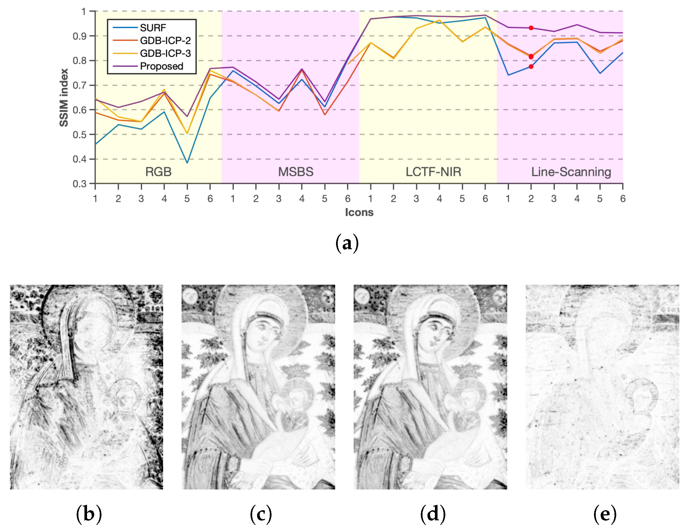
Figure 15.
The estimated SNRs of the gray patches in the Macbeth color chart, plotted for each channel of: (a) Nikon D80 camera; (b) FluxData MSBS camera; and (c) LCTF-VIS camera. The values in (c) are reordered and plotted for each patch in (d).
Figure 15.
The estimated SNRs of the gray patches in the Macbeth color chart, plotted for each channel of: (a) Nikon D80 camera; (b) FluxData MSBS camera; and (c) LCTF-VIS camera. The values in (c) are reordered and plotted for each patch in (d).

© 2019 by the author. Licensee MDPI, Basel, Switzerland. This article is an open access article distributed under the terms and conditions of the Creative Commons Attribution (CC BY) license (http://creativecommons.org/licenses/by/4.0/).
Share and Cite
MDPI and ACS Style
Mirhashemi, A. Configuration and Registration of Multi-Camera Spectral Image Database of Icon Paintings. Computation 2019, 7, 47. https://doi.org/10.3390/computation7030047
AMA Style
Mirhashemi A. Configuration and Registration of Multi-Camera Spectral Image Database of Icon Paintings. Computation. 2019; 7(3):47. https://doi.org/10.3390/computation7030047
Chicago/Turabian StyleMirhashemi, Arash. 2019. "Configuration and Registration of Multi-Camera Spectral Image Database of Icon Paintings" Computation 7, no. 3: 47. https://doi.org/10.3390/computation7030047
Note that from the first issue of 2016, this journal uses article numbers instead of page numbers. See further details here.