Article

Estimating the Entropy of Binary Time Series: Methodology, Some Theory and a Simulation Study

1
Knight Equity Markets, L.P., Jersey City, NJ 07310, USA
2
Department of Informatics, Athens University of Economics and Business, Athens 10434, Greece
3
Division of Applied Mathematics and Department of Neuroscience, Brown University, Providence, RI 02912, USA
*
Author to whom correspondence should be addressed.
Entropy 2008, 10(2), 71-99; https://doi.org/10.3390/entropy-e10020071
Submission received: 6 March 2008 / Revised: 9 June 2008 / Accepted: 17 June 2008 / Published: 17 June 2008

Abstract

:
Partly motivated by entropy-estimation problems in neuroscience, we present a detailed and extensive comparison between some of the most popular and effective entropy estimation methods used in practice: The plug-in method, four different estimators based on the Lempel-Ziv (LZ) family of data compression algorithms, an estimator based on the Context-Tree Weighting (CTW) method, and the renewal entropy estimator. Methodology: Three new entropy estimators are introduced; two new LZ-based estimators, and the “renewal entropy estimator,” which is tailored to data generated by a binary renewal process. For two of the four LZ-based estimators, a bootstrap procedure is described for evaluating their standard error, and a practical rule of thumb is heuristically derived for selecting the values of their parameters in practice. Theory: We prove that, unlike their earlier versions, the two new LZ-based estimators are universally consistent, that is, they converge to the entropy rate for every finite-valued, stationary and ergodic process. An effective method is derived for the accurate approximation of the entropy rate of a finite-state hidden Markov model (HMM) with known distribution. Heuristic calculations are presented and approximate formulas are derived for evaluating the bias and the standard error of each estimator. Simulation: All estimators are applied to a wide range of data generated by numerous different processes with varying degrees of dependence and memory. The main conclusions drawn from these experiments include:  For all estimators considered, the main source of error is the bias. (ii) The CTW method is repeatedly and consistently seen to provide the most accurate results. (iii) The performance of the LZ-based estimators is often comparable to that of the plug-in method. (iv) The main drawback of the plug-in method is its computational inefficiency; with small word-lengths it fails to detect longer-range structure in the data, and with longer word-lengths the empirical distribution is severely undersampled, leading to large biases.

1. Introduction

The problem of estimating the entropy of a sequence of discrete observations has received a lot of attention over the past two decades. A, necessarily incomplete, sample of the theory that has been developed can be found in [1,2,3,4,5,6,7,8,9,10,11,12,13,14] and the references therein. Examples of numerous different applications are contained in the above list, as well as in [15,16,17,18,19,20,21,22,23,24,25,26,27].
Information-theoretic methods have been particularly widely used in neuroscience, in a broad effort to analyze and understand the fundamental information-processing tasks performed by the brain. In many of these studies, the entropy is adopted as the main measure for describing the amount of information transmitted between neurons. There, the continuous signal describing the sequence of action potentials is typically quantized in time (into bins of duration in the order of milliseconds), and each bin is labelled 1 or 1, according to whether or not a action potential, or “spike” occurred in that time interval. One of the most basic tasks in this area is to identify appropriate methods for quantifying this information, in other words, to estimate the entropy of spike trains recorded from live animals; see, e.g., [13,18,20,24,25,26,27,28,29,30,31].
Motivated, in part, by the application of entropy estimation techniques to such neuronal data, we present a systematic and extensive comparison, both in theory and via simulation, between several of the most commonly used entropy estimation techniques. This work serves, partly, as a more theoretical companion to the experimental work and results presented in [32,33,34]. There, entropy estimators were applied to the spike trains of 28 neurons recorded simultaneously for a one-hour period from the primary motor and dorsal premotor cortices (MI, PMd) of a monkey. The purpose of those experiments was to examine the effectiveness of the entropy as a statistic, and its utility in revealing some of the underlying structural and statistical characteristics of the spike trains. In contrast, our main aim here is to examine the performance of several of the most effective entropy estimators, and to establish fundamental properties for their applicability, such as rigorous estimates for their convergence rates, bias and variance. In particular, since (discretized) spike trains are typically represented as binary sequences [35], some of our theoretical results and all of our simulation experiments are focused on binary data.
Section 2 begins with a description of the entropy estimators we consider. The simplest one is the plug-in or maximum likelihood estimator, which consists of first calculating the empirical frequencies of all words of a fixed length in the data, and then computing the entropy of this empirical distribution. For obvious computational reasons, the plug-in is ineffective for word-lengths beyond 10 or 20, and hence it cannot take into account any potential longer-time dependencies in the data.
A popular approach for overcoming this drawback is to consider entropy estimators based on “universal” data compression algorithms, that is, algorithms which are known to achieve a compression ratio equal to the entropy, for data generated by processes which may possess arbitrarily long memory, and without any prior knowledge about the distribution of the underlying process. Since, when trying to estimate the entropy, the actual compression task is irrelevant, many entropy estimators have been developed as modifications of practical compression schemes. Section 2.3 describes two well-known such entropy estimators [9], which are based on the Lempel-Ziv (LZ) family of data compression algorithms [36,37]. These estimators are known to be consistent (i.e., to converge to the correct value for the entropy) only under certain restrictive conditions on the data. We introduce two new LZ-based estimators, and we prove in Theorem 2.1 that, unlike the estimators in [9], they are consistent under essentially minimal conditions, that is, for data generated by any stationary and ergodic process.
Section 2.4 contains an analysis, partly rigorous and partly in terms of heuristic computations, of the rate at which the bias and the variance of each of the four LZ-based estimators converges to zero. A bootstrap procedure is developed for empirically estimating the standard error of two of the four LZ-based estimators, and a practical rule-of-thumb is derived for selecting the values of the parameters of these estimators in practice.
Next, in Section 2.5 we consider an entropy estimator based on the Context-Tree Weighting (CTW) algorithm [38,39,40]. [In the neuroscience literature, a similar proceedure has been applied in [29] and [25].] The CTW, also originally developed for data compression, can be interpreted as a Bayesian estimation procedure. After a brief description, we explain that it is consistent for data generated by any stationary and ergodic process and show that its bias and variance are, in a sense, as small as can be.*
Section 3 contains the results of an extensive simulation study, where the various entropy estimators are applied to data generated from numerous different types of processes, with varying degrees of dependence and memory. In Section 3.1, after giving brief descriptions of all these data models, we present (Proposition 3.1) a method for accurately approximating the entropy rate of a Hidden Markov Model (HMM); recall that HMMs are not known to admit closed-form expressions for their entropy rate. Also, again partly motivated by neuroscience applications, we introduce another new entropy estimator, the renewal entropy estimator, which is tailored to binary data generated by renewal processes.
Section 3.2 contains a detailed examination of the bias and variance of the four LZ-based estimators and the CTW algorithm. There, our earlier theoretical predictions are largely confirmed. Moreover, it is found that two of the four LZ-based estimators are consistently more accurate than the other two.
Finally, Section 3.3 contains a systematic comparison of the performance of all of the above estimators on different types of simulated data. Incidental comparisons between some of these methods on limited data sets have appeared in various places in the literature, and questions have often been raised regarding their relative merits. One of the main goals of the work we report here is to offer clear resolutions for many of these issues. Specifically, in addition to the points mentioned up to now, some of the main conclusion that we draw from the simulation results of Section 3 (these and more are collected in Section 4) can be summarized as follows:
  • Due its computational inefficiency, the plug-in estimator is the least reliable method, in contrast to the LZ-based estimators and the CTW, which naturally incorporate dependencies in the data at much larger time scales.
  • The most effective estimator is the CTW method. Moreover, for the CTW as well as for all other estimators, the main source of error is the bias and not the variance.
  • Among the four LZ-based estimators, the two most efficient ones are those with increasing win- dow sizes, Ĥn of [9] and H ^ n introduced in Section 2.3. Somewhat surprisingly, in several of the simulations we conducted the performance of the LZ-based estimators appears to be very similar to that of the plug-in method.

2. Entropy Estimators and Their Properties

This section contains a detailed description of the entropy estimators that will be applied to simulated data in Section 3. After some basic definitions and notation in Section 2.1, the following four subsections contain the definitions of the estimators together with a discussion of their statistical properties, including conditions for consistency, and estimates of their bias and variance.

2.1. Entropy and Entropy Rate

Let X be a random variable or random vector, taking values in an arbitrary finite set A, its alphabet, and with distribution p(x) = Pr{X = x} for xA. The entropy of X [41] is defined as,
H ( X ) = H ( p ) = x A p ( x ) log p ( x ) ,
where, throughout the paper, log denotes the logarithm to base 2, log2. A random process X = {. . . , X−1, X0, X1, X2, . . .} with alphabet A is a sequence of random variables {Xn} with values in A. We write X i j = (Xi, Xi+1, . . . , Xj) for a (possibly infinite) contiguous segment of the process, with −∞ ≤ ij ≤ ∞, and x i j = (xi, xi+1, . . . , xj) for a specific realization of X i j , so that x i j is an element of Aj−i+1. The entropy rate H = H(X), or “per-symbol” entropy, of X is the asymptotic rate at which the entropy of X 1 n changes with n,
H = H ( X ) = lim n 1 n H ( X 1 , X 2 , , X n ) ,
whenever the limit exists, where H(X1, X2, . . . , Xn) is the entropy of the jointly distributed random variables X 1 n = (X1, X2, . . . , Xn). Recall [41] that for a stationary process (i.e., a process such that the distribution of every finite block X n + 1 n + k of size k has the same distribution, say pk , independently of its position n), the entropy rate exists and equals,
H = H ( X ) = lim n H ( X n | X n 1 , , X 2 , X 1 ) ,
where the conditional entropy H ( X n | X 1 n 1 ) = H ( X n | X n 1 , , X 2 , X 1 ) is defined as,
Entropy 10 00071 i001
As mentioned in the introduction, much of the rest of the paper will be devoted to binary data produced by processes X with alphabet A = {0. 1}.

2.2. The Plug-in Estimator

Perhaps the simplest and most straightforward estimator for the entropy rate is the so-called plug-in estimator. Given a data sequence x 1 n of length n, and an arbitrary string, or “word,” y 1 w Aw of length w < n, let p ^ w ( y 1 w ) denote the empirical probability of the word y 1 w in x 1 n ; that is, p ^ w ( y 1 w ) is the frequency with which y 1 w appears in x 1 n . If the data are produced from a stationary and ergodicprocess, then the law of large numbers guarantees that, for fixed w and large n, the empirical distribution p ^ w will be close to the true distribution pw, and therefore a natural estimator for the entropy rate based on (1) is:
H ^ n , w , plug in = 1 w H ( p ^ w ) = 1 w y 1 w A w p ^ w ( y 1 w ) log p ^ w ( y 1 w ) .
This is the plug-in estimator with word-length w. Since the empirical distribution is also the maximum likelihood estimate of the true distribution, this is also often referred to as the maximum-likelihood entropy estimator.
Suppose the process X is stationary and ergodic. Then, taking w large enough for 1 w H ( X 1 w ) to beacceptably close to H in (1), and assuming the number of samples n is much larger than w so that the empirical distribution of order w is close to the true distribution, the plug-in estimator Ĥn,w,plug−in will produce an accurate estimate for the entropy rate. But, among other difficulties, in practice this leads to enormous computational problems because the number of all possible words of length w grows exponentially with w. For example, even for the simple case of binary data with a modest word-length of w = 30, the number of possible strings y 1 w is 230, which in practice means that the estimator would either require astronomical amounts of data to estimate p ^ w accurately, or it would be severely undersampled. See also [43] and the references therein for a discussion of the undersampling problem.
Another drawback of the plug-in estimator is that it is hard to quantify its bias and to correct for it. For any fixed word-length w, it is easy to see that the bias E[Ĥn,w,plug−in] − 1 w H ( X 1 w ) ) is always negative [12,13], whereas the difference between the wth-order per-symbol entropy and the entropy rate, 1 w H ( X 1 w ) ) − H(X). is always nonnegative. Still, there have been numerous extensive studies on calculating this bias and on developing ways to correct for it; see [13,18,20,24,27,28] and the references therein.

2.3. The Lempel-Ziv Estimators

An intuitively appealing and popular way of estimating the entropy of discrete data with possibly long memory, is based on the use of so-called universal data compression algorithms. These are algorithms that are known to be able to optimally compress data from an arbitrary process (assuming some broad conditions are satisfied), where optimality means that the compression ratio they achieve is asymptotically equal to the entropy rate of the underlying process – although the statistics of this process are not assumed to be known a priori. Perhaps the most commonly used methods in this context are based on a family of compression schemes known as Lempel-Ziv (LZ) algorithms; see, e.g., [36,37,44].
Since the entropy estimation task is simpler than that of actually compressing the data, several modified versions of the original compression algorithms have been proposed and used extensively in practice. All these methods are based on the calculation of the lengths of certain repeating patterns in the data. Specifically, given a data realization x = (. . . , x−1, x0, x1, x2, . . .), for every position i in x and any “window length” n ≥ 1, consider the length of the longest segment x i i + + 1 in the data starting at i which also appears in the window x i n i 1 of length n preceding position i. Formally, define L i n = L i n ( x ) = L i n ( x i n i + n 1 ) as 1+ [that longest match-length]:
Entropy 10 00071 i002
Suppose that the process X is stationary and ergodic, and consider the random match-lengths L i n = L i n ( X i n i + n 1 ) . In [44,45] it was shown that, for any fixed position i, the match-lengths grow logarithmically with the window size n, and in fact,
Entropy 10 00071 i003
where H is the entropy rate of the process. This result suggests that the quantity (log n)/ L i n can be used as an entropy estimator, and, clearly, in order to make more efficient use of the data and reduce the variance, it would be more reasonable to look at the average value of various match-lengths L i n taken at different positions i; see the discussion in [9]. To that effect, the following two estimators are considered in [9]. Given a data realization x = x , a window length n ≥ 1, and a number of matches k ≥ 1, the sliding-window LZ estimator Ĥn,k = Ĥn,k(x) = Ĥn,k( x n + 1 n + k 1 ) is defined by,
Entropy 10 00071 i004
Similarly, the increasing-window LZ estimator Ĥn = Ĥn(x) = Ĥn( x 0 2 n 1 ) is defined by,
Entropy 10 00071 i005
The difference between the two estimators in (3) and (4) is that Ĥn,k uses a fixed window length, while Ĥn uses the entire history as its window, so that the window length increases as the matching position moves forward.
In [9] it is shown that, under appropriate conditions, both estimators Ĥn,k and Ĥn are consistent, in that they converge to the entropy rate of the underlying process with probability 1, as n, k → ∞. Specifically, it is assumed that the process is stationary and ergodic, that it takes on only finitely many values, and that it satisfies the Doeblin Condition (DC). This condition says that there is a finite number of steps, say r, in the process, such that, after r time steps, no matter what has occurred before, anything can happen with positive probability:
Doeblin Condition (DC).
There exists an integer r ≥ 1 and a real number β > 0 such that,
Pr ( X r = a | X 0 ) > β
for all aA and with probability one in the conditioning, i.e., for almost all semi-infinite realizations of the past X 0 = ( X 0 , X 1 , ) .
Condition (DC) has the advantage that it is not quantitative – the values of r and β can be arbitrary – and, therefore, for specific applications it is fairly easy to see whether it is satisfied or not. But it is restrictive, and, as it turns out, it can be avoided altogether if we consider a modified version of the above two estimators.
To that end, we define two new estimators H ~ n , k and H ~ n as follows. Given x = x , n and k as above, define the new sliding-window estimator H ~ n , k = H ~ n , k ( x ) = H ~ n , k ( x n + 1 n + k 1 ) ,
Entropy 10 00071 i006
and the new increasing-window estimator H ~ n = H ~ n ( x ) = H ~ n ( x 0 2 n 1 ) as,
Entropy 10 00071 i007
Below some basic properties of these four estimators are established, and conditions are given for their asymptotic consistency. Parts (i) and (iii) of Theorem 2.1 are new; most of part (ii) is contained in [9].
Theorem 2.1.
[Consistency of LZ-type Estimators]
(i)
When applied to an arbitrary data string, the estimators defined in (3)–(6) always satisfy,
H ^ n , k H ~ n , k   a n d   H ^ n H ~ n ,
for any n, k.
(ii)
The estimators Ĥn,k and Ĥn are consistent when applied to data generated by a finite-valued, stationary, ergodic process that satisfies Doeblin’s condition (DC). With probability one we have:
Ĥn,kH, ĤnH,   as k, n → ∞.
(iii)
The estimators H ~ n , k and H ~ n are consistent when applied to data generated by an arbitrary finite-valued, stationary, ergodic process, even if (DC) does not hold. With probability one we have:
H ~ n , n H ,   H ~ n H ,     a s   k , n .
Note that parts (ii) and (iii) do not specify the manner in which n and k go to infinity. The results are actually valid in the following cases:
  • If the two limits as n and k tend to infinity are taken separately, i.e., first k → ∞ and then n → ∞, or vice versa;
  • If k → ∞ and n = nk varies with k in such a way that nk → ∞ as k → ∞;
  • If n → ∞ and k = kn varies with n in such a way that it increases to infinity as n → ∞;
  • If k and n both vary arbitrarily in such a way that k stays bounded and n → ∞.
Proof. 
Part (i). An application of Jensen’s inequality to the convex function x ↦ 1/x, with respect to the uniform distribution (1/k,. . . , 1/k) on the set {1, 2, . . . , k}, yields,
Entropy 10 00071 i008
as required. The proof of the second assertion is similar.
Part (ii). The results here are, for the most part, proved in [9], where it is established that ĤnH and Ĥn,nH as n → ∞, with probability one. So it remains to show that Ĥn,kH as n, k → ∞ in each of the four cases stated above.
For case 1 observe that, with probability 1,
Entropy 10 00071 i009
where (a) follows from (2). To reverse the limits, we define, for each fixed n, a new process { Y i ( n ) } = { , Y 1 ( n ) , Y 0 ( n ) , Y 1 ( n ) , Y 2 ( n ) , } by letting Y i ( n ) = L i n /(log n) for each i. Then the process { Y i ( n ) } is itself stationary and ergodic. Recalling also from [9] that the convergence in (2) takes place not only with probability one but also in L1, we may apply the ergodic theorem to obtain that, with probability 1,
Entropy 10 00071 i010
where (b) follows by the ergodic theorem and (c) from the L1 version of (2).
The proof of case 2 is identical to the case k = n considered in [9]. In case 3, since the sequence {kn} is increasing, the limit of Hkn,n reduces to a subsequence of the corresponding limit in case 2 upon considering the inverse sequence {nk}.
Finally for case 4, recall from (7) that,
lim n H k , n = H   with prob .   1 ,
for any fixed k. Therefore the same will hold with a varying k, as long as it varies among finitely many values.
Part (iii). The proofs of the consistency results for H ~ n and H ~ n , k can be carried out along the same lines as the proofs of the corresponding results in [9], together with their extensions as in Part (ii) above. The only difference is in the main technical step, namely, the verification of a uniform integrability condition. In the present case, what is needed is to show that,
Entropy 10 00071 i011
This is done in the following lemma. ☐
Lemma 2.1.
Under the assumptions of part (iii) of the theorem, the L1-domination condition (8) holds true.
Proof. 
Given a data realization x = (. . . , x−2, x−1, x0, x1, x2, . . .) and an m ≥ 1, the recurrence time Rm is defined as the first time the substring x 1 m appears again in the past. More precisely, Rm is the number of steps to the left of x 1 m we have to look in order to find a copy of x 1 m :
R m = R m ( x ) = R m ( x m ) = inf { k 1 : x 1 m = x k + 1 k + m } .
For any such realization x and any n ≥ 1, if we take m = L 1 n , then by the definitions of Rm and L 1 n it follows that, Rm > n, which implies,
log R m m > log n L 1 n ,
and thus it is always the case that,
sup n log n L 1 n < sup m log R m m .
Therefore, to establish (8) it suffices to prove:
E { sup m log R m m } < .
To that end, we expand this expectation as,
Entropy 10 00071 i012
where K is an arbitrary integer to be chosen later. Applying Markov’s inequality,
E { sup m log R m m } K + k K m 1 E ( R m ) 2 m k .
To calculate the expectation of Rm, suppose that the process X takes on α = |A| possible values, so that there are αm possible strings x 1 m of length m. Now recall Kac’s theorem [44] which states that E ( R m | X 1 m = x 1 m ) = 1 / Pr { X 1 m = x 1 m } , from which it follows that,
E ( R m ) = x 1 m E ( R m | X 1 m = x 1 m ) Pr { X 1 m = x 1 m } = α m .
Combining (10) and (11) yields,
Entropy 10 00071 i013
where we choose K > log α. This establishes (9) and completes the proof.      ☐

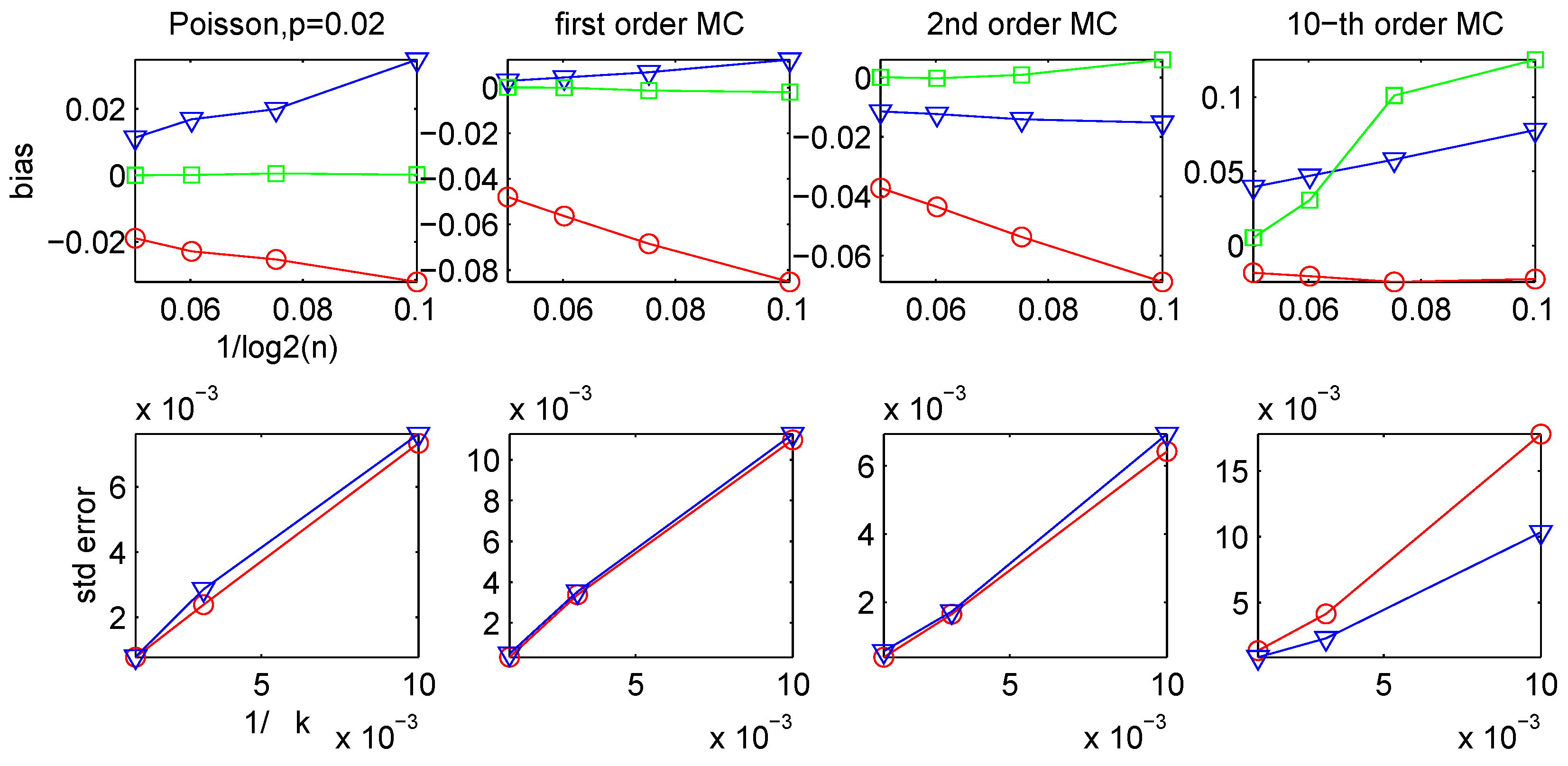
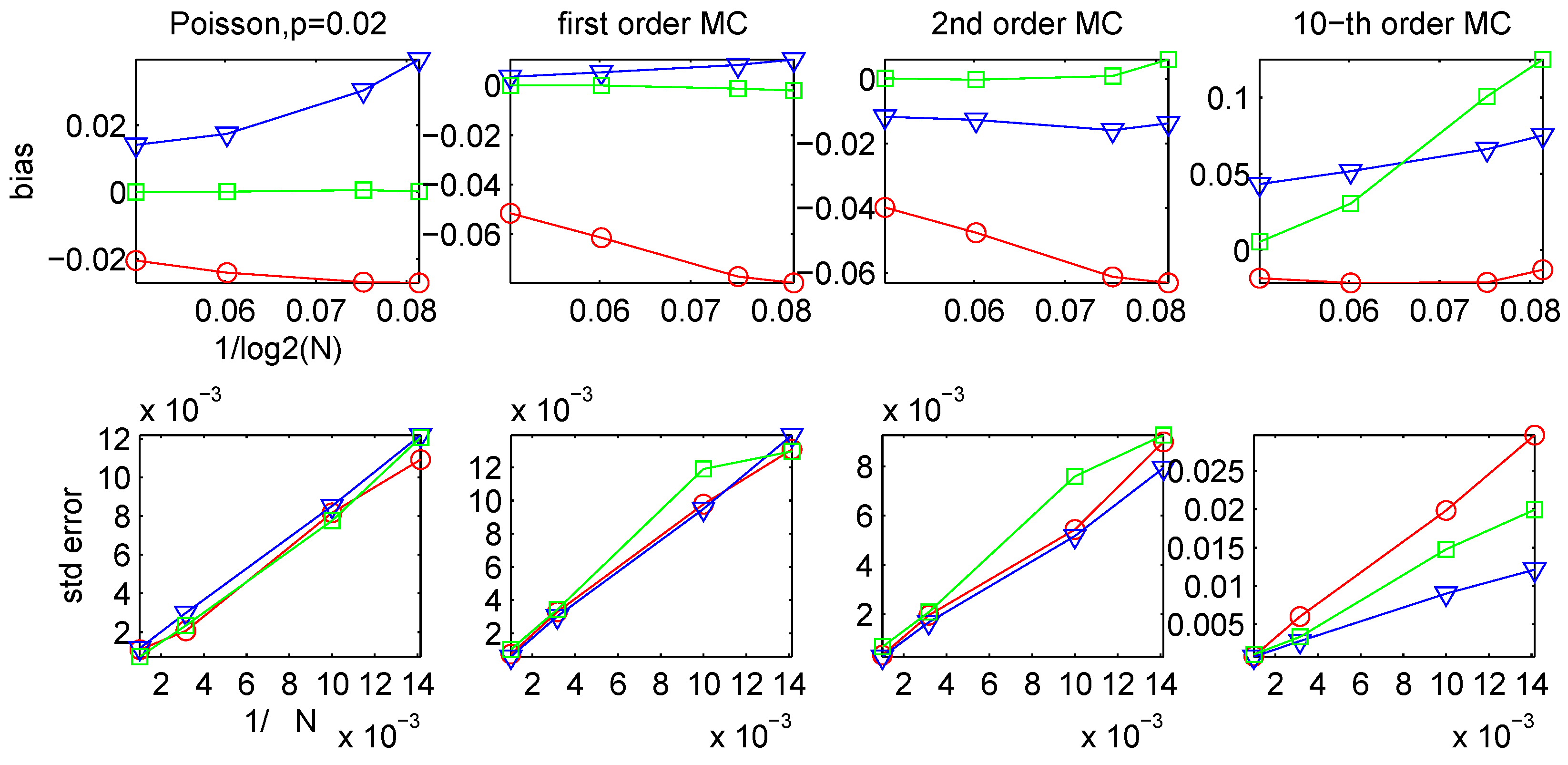
2.4. Bias and Variance of the LZ-based Estimators

In practice, when applying the sliding-window LZ estimators Ĥn,k or H ~ n , k on finite data strings, the values of the parameters k and n need to be chosen, so that k + n is approximately equal to the total data length. This presents the following dilemma: Using a long window size n, the estimators are more likely to capture the longer-term trends in the data, but, as shown in [46,47], the match-lengths L i n starting at different positions i have large fluctuations. So a large window size n and a small number of matching positions k will give estimates with high variance. On the other hand, if a relatively small value for n is chosen and the estimate is an average over a large number of positions k, then the variance will be reduced at the cost of increasing the bias, since the expected value of L i n /log n is known to converge to 1/H very slowly [48].
Therefore n and k need to be chosen in a way such that the above bias/variance trade-off is balanced. From the earlier theoretical results of [46,47,48,49,50] it follows that, under appropriate conditions, the bias is approximately of the order O(1/log n), whereas from the central limit theorem it is easily seen that the variance is approximately of order O(1/k). This indicates that the relative values of n and k should probably be chosen to satisfy kO((log n)2).
Although this is a useful general guideline, we also consider the problem of empirically evaluating the relative estimation error on particular data sets. Next we outline a bootstrap procedure, which gives empirical estimates of the variance Ĥn,k and H ~ n , k ; an analogous method was used for the estimator Ĥn,k in [21], in the context of estimating the entropy of whale songs.
Let L denote the sequence of match-lengths L = ( L 1 n , , L 2 n , , L k n ) computed directly from the data, as in the definitions of Ĥn,k and H ~ n , k . Roughly speaking, the proposed procedure is carried out in three steps: First, we sample with replacement from L in order to obtain many pseudo-time series with the same length as L; then we compute new entropy estimates from each of the new sequences using Ĥn,k or H ~ n , k ; and finally we estimate the variance of the initial entropy estimates as the sample variance of the new estimates. The most important step is the sampling, since the elements of sequence ( L 1 n , , L k n ) are not independent. In order to maintain the right form of dependence, we adopt a version of the stationary bootstrap procedure of [51]. The basic idea is, instead of sampling individual L i n ’s from L, to sample whole blocks with random lengths. The choice of the distribution of their lengths is made in such a way as to guarantee that they are typically long enough to maintain sufficient dependence as in the original sequence. The results in [51] provide conditions which justify the application of this procedure.
The details of the three steps above are as follows: First, a random position j ∈ {1, 2, . . . , k} is selected uniformly at random, and a random length T is chosen with geometric distribution with mean 1/p (the choice of p is discussed below). Then the block of match-lengths ( L j n , L j + 1 n , , L j + T 1 ) copied from L, and the same process is repeated until the concatenation L* of the sampled blocks has length k. This gives the first bootstrap sample. Then the whole process is repeated to generate a total of B such blocks L*1, L*2, . . . , L*B, each of length k. From these we calculate new entropy estimates Ĥ *(m) or H ~ *(m), for m = 1, 2, . . . , B, according to the definition of the entropy estimator being used, as in (3) or (5), respectively; the choice of the number B of blocks is discussed below. The bootstrap estimate of the variance of Ĥ is,
σ ^ 2 = 1 B 1 m = 1 B [ H ^ * ( m ) μ ^ ] 2 ,
where μ ^ = B 1 m = 1 B H ^ * ( m ) similarly for H ~ .
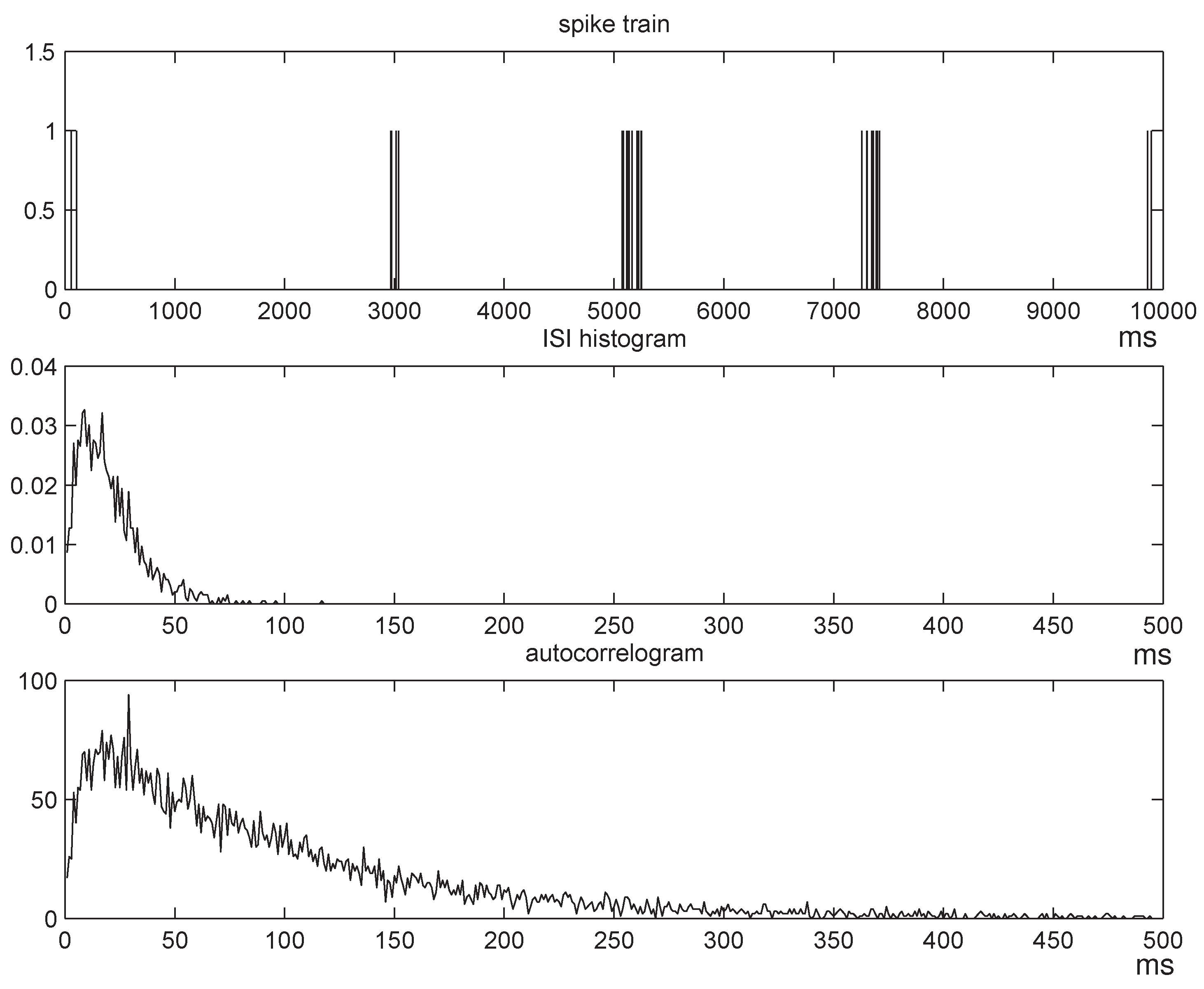
The choice of the parameter p depends on the length of the memory of the match-length sequence L = ( L 1 n , , L 2 n , , L k n ) ; the longer the memory, the larger the blocks need to be, therefore, the smaller the parameter p. In practice, p is chosen by studying the autocorrelogram of L, which is typically decreasing with the lag: We choose an appropriate cutoff threshold, take the corresponding lag to be the average block size, and choose p as the reciprocal of that lag. Finally, the number of blocks B is customarily chosen large enough so that the histogram of the bootstrap samples Ĥ *(1), Ĥ *(2), . . . , Ĥ *(B) “looks” approximately Gaussian. Typical values used in applications are between B = 500 and B = 1000. In all our experiments in [33,34] and in the results presented in the following section we set B = 1000, which, as discussed below, appears to have been sufficiently large for the central limit theorem to apply to within a close approximation.

2.5. Context-Tree Weighting

One of the fundamental ways in which the entropy rate arises as a natural quantity, is in the Shannon- McMillan-Breiman theorem [41]; it states that, for any stationary and ergodic process
X = {. . . , X−1, X0, X1, X2, . . .},
with entropy rate H,
1 n log p n ( X 1 n ) H ,     with prob.   1 ,   as n   ,
where p n ( X 1 n ) denotes the (random) probability of the random string X 1 n . This suggests that, one way to estimate H from a long realization x 1 n of X, is to first somehow estimate its probability and then use the estimated probability p ^ n ( x 1 n ) to obtain an estimate for the entropy rate via,
H ^ n , est = 1 n log p ^ n ( x 1 n ) .
The Context-Tree Weighting (CTW) algorithm [38,39,40] is a method, originally developed in the context of data compression, which can be interpreted as an implementation of hierarchical Bayesian procedure for estimating the probability of a string generated by a binary “tree process.”The details of the precise way in which the CTW operates can be found in [38,39,40]; here we simply give a brief overview of what (and not how) the CTW actually computes. In order to do that, we first need to describe tree processes.
A binary tree process of depth D is a binary process X with a distribution defined in terms of a suffix set S, consisting of binary strings of length no longer than D, and a parameter vector θ = (θs; sS), where each θs ∈ [0, 1]. The suffix set S is assumed to be complete and proper, which means that any semi-infinite binary string x 0 has exactly one suffix s is S, i.e., there exists exactly one sS such that x 0 can be written as x k s, for some integer k.§We write s = s( x 0 ) ∈ S for this unique suffix.
Then the distribution of X is specified by defining the conditional probabilities,
Pr { X n + 1 = 1 | X n = x n } = 1 Pr { X n + 1 = 0 | X n = x n } = θ s ( x n ) .
It is clear that the process just defined could be thought of simply as a D-th order Markov chain, but this would ignore the important information contained in S: If a suffix string sS has length < D, then, conditional on any past sequence x n which ends in s, the distribution of Xn+1 only depends on the most recent symbols. Therefore, the suffix set offers an economical way for describing the transition probabilities of X, especially for chains that can be represented with a relatively small suffix set.
Suppose that a certain string x 1 n has been generated by a tree process of depth no greater than D, but with unknown suffix set S* and parameter vector θ* = (θ*s; sS). Following classical Bayesian methodology, we assign a prior probability π(S) on each (complete and proper) suffix set S of depth D or less, and, given S, we assign a prior probability π(θ|S) on each parameter vector θ = (θs). A Bayesian approximation to the true probability of x 1 n (under S* and θ*) is the mixture probability,
Entropy 10 00071 i014
where PS,θ( x 1 n ) is the probability of x 1 n under the distribution of a tree process with suffix set S and parameter vector θ. The expression in (14) is, in practice, impossible to compute directly, since the number of suffix sets of depth ≤ D (i.e., the number of terms in the sum) is of order 2D. This is obviously prohibitively large for any D beyond 20 or 30.
The CTW algorithm is an efficient procedure for computing the mixture probability in (14), for a specific choice of the prior distributions π(S), π(θ|S): The prior on S is,
π(S) = 2−|S|−N(S)+1,
where |S| is the number of elements of S and N (S) is the number of strings in S with length strictly smaller than D. Given a suffix set S, the prior on θ is the product ( 1 2 , 1 2 ) -Dirichlet distribution, i.e., under π(θ|S) the individual θs are independent, with each θs ∼ Dirichlet ( 1 2 , 1 2 ) .
The main practical advantage of the CTW algorithm is that it can actually compute the probability in (14) exactly. In fact, this computation can be performed sequentially, in linear time in the length of the string n, and using an amount of memory which also grows linearly with n. This, in particular, makes it possible to consider much longer memory lengths D than would be possible with the plug-in method.
The CTW Entropy Estimator.
Thus motivated, given a binary string x 1 n , we define the CTW entropy estimator Ĥn,D, ctw as,
H ^ n , D , ctw = 1 n log P ^ D , mix ( x 1 n ) ,
Where P ^ D , m i x ( x 1 n ) is the mixture probability in (14) computed by the CTW algorithm. [Corresponding proceedures are similarly described in [25,29].] The justification for this definition comes from the discussion leading to equation (13) above. Clearly, if the true probability of x 1 n is P*( x 1 n ), the estimator performs well when,
1 n log P ^ D , mix ( x 1 n ) 1 n log P * ( x 1 n ) .
In many cases this approximation can be rigorously justified, and in certain cases it can actually be accurately quantified.
Assume that x 1 n is generated by an unknown tree process (of depth no greater than D) with suffix set S*. The main theoretical result of [38] states that, for any string x 1 n , of any finite length n, generated by any such process, the difference between the two terms in (16) can be uniformly bounded above; from this it easily follows that,
1 n log P ^ D , mix ( x 1 n ) [ 1 n log P * ( x 1 n ) ] | S * | 2 n log n + 3 | S * | + 1 n .
This nonasymptotic, quantitative bound, easily leads to various properties of Ĥn,D, ctw:
First, (17) combined with the Shannon-McMillan-Breiman theorem (12) and the pointwise converse source coding theorem [52,53], readily implies that ĤN,D, ctw is consistent, that is, it converges to the true entropy rate of the underlying process, with probability one, as n → ∞. Also, Shannon’s source coding theorem [41] implies that the expected value of Ĥn,D,ctw cannot be smaller than the true entropy rate H; therefore, taking expectations in (17) gives,
0 [ bias   of   p ^ n , D , ctw ] | S | 2 n log n + O ( 1 ) .
In view of Rissanen’s [54] well-known universal lower bound, (18) shows that the bias of the CTW is essentially as small as can be. Finally, for the variance, if we subtract H from both sides of (17), multiply by n , and apply the central-limit refinement to the Shannon-McMillan-Breiman theorem [55,56], we obtain that the standard deviation of the estimates H ^ n , D , is σ X / n , where σ X 2 is the minimal coding variance of X [57]. This is also optimal, in view of the second-order coding theorem of [57].
Therefore, for data x 1 n generated by an arbitrary tree processes, the bias of the CTW estimator is of order O(log n/n), and its variance is O(1/n). Compared to the earlier LZ-based estimators, these bounds suggest much faster convergence, and are in fact optimal. In particular, the O(log n/n) bound on the bias indicates that, unlike the LZ-based estimators, the CTW can give useful results even on small data sets.
Extensions. 
An important issue for the performance of the CTW entropy estimator, especially when used on data with potentially long-range dependence, is the choice of the depth D: While larger values of D give the estimator a chance to capture longer-term trends, we then pay a price in the algorithm’s complexity and in the estimation bias. This issue will not be discussed further here; a more detailed discussion of this point along with experimental results can be found in [33,34].
The CTW algorithm has also been extended beyond finite-memory processes [40]. The basic method is modified to produce an estimated probability P ^ ( x 1 n ) , without assuming a predetermined maximal suffix depth D. The sequential nature of the computation remains exactly the same, leading to a corresponding entropy estimator defined analogously to the one in (15), as H ^ n , , ctw = 1 n log P ^ ( x 1 n ) . Again it is easy to show that Ĥn,∞,ctw is consistent with probability one, this time for every stationary and ergodic (binary) process. The price of this generalization is that the earlier estimates for the bias and variance no longer apply, although they do remain valid is the data actually come from a finite-memory process. In numerous simulation experiments we found that there is no significant advantage in using Ĥn,D,ctw with a finite depth D over Ĥn,∞,ctw, except for the somewhat shorter computation time. For that reason, in all the experimental results in Section 3.2 and Section 3.3 below, we only report estimates obtained by Ĥn,∞,ctw.
Finally, perhaps the most striking feature of the CTW algorithm is that it can be modified to compute the “best” suffix set S that can be fitted to a given data string, where, following standard statistical (Bayesian) practice, “best” here means the one which is most likely under the posterior distribution. To be precise, recall the prior distributions π(S) and π(θ|S) on suffix sets S and on parameter vectors θ, respectively. Using Bayes’ rule, the posterior distribution on suffix sets S can be expressed,
Entropy 10 00071 i015
the suffix set S ^ = S ^ ( x 1 n ) which maximizes this probability is called the Maximum A posteriori Probability, or MAP, suffix set. Although the exact computation of Ŝ is, typically, prohibitively hard to carry out directly, the Context-Tree Maximizing (CTM) algorithm proposed in [58] is an efficient procedure (with complexity and memory requirements essentially identical to the CTW algorithm) for computing Ŝ. The CTM algorithm will not be used or discussed further in this work; see the discussion in [33,34], where it plays an important part in the analysis of neuronal data.

3. Results on Simulated Data

This section contains the results of an extensive simulation study, comparing various aspects of the behavior of the different entropy estimators presented earlier (the plug-in estimator, the four LZ-based estimators, and the CTW estimator), applied to different kinds of simulated binary data. Motivated, in part, by applications in neuroscience, we also introduce a new method, the renewal entropy estimator. Section 3.1 contains descriptions of the statistical models used to generate the data, along with exact formulas or close approximations for their entropy rates.
Section 3.2 and Section 3.3 contain the actual simulation results.

3.1 Statistical Models and Their Entropy Rates

3.1.1 I.I.D. (or “homogeneous Poisson”) Data

The simplest model of a binary random process X is as a sequence of independent and identically distributed (i.i.d.) random variables {Xn}, where the Xi are independent and all have the same distribution. This process has no memory, and in the neuroscience literature it is often referred to as a “homogeneous Poisson process” (since sampling a Poisson process at regular time intervals and replacing the sampled values by their successive differences produces such an i.i.d. sequence). The distribution of each Xi is described by a parameter p ∈ [0, 1], so that Pr{Xi = 1} = p and Pr{Xi = 0} = 1 − p. If {Xn} were to represent a spike train, then p = E(Xi) would be its average firing rate.
The entropy rate of this process is simply,
H = H(X1) = −p log p − (1 − p) log(1 − p).

3.1.2. Markov Chains

An -th order (homogeneous) Markov chain with (finite) alphabet A is a process X = {Xn} with the property that,
Pr { X n = x n | X 1 n 1 = x 1 n 1 } = Pr { X n = x n | X n n = x n n } = P x n n , x n ,
for all x 1 n A n , where P = ( P x 1 , x + 1 ) is the transition matrix of the chain. This formalizes the idea that the memory of the process has length : The probability of each new symbol depends only on the most recent symbols, and it is conditionally independent of the more distant past. The distribution of this process is described by the initial distribution of its first symbols, (π( x 1 )), and the transition matrix P. The entropy rate of an ergodic (i.e., irreducible and aperiodic) -th order Markov chain X is given by,
H = x 1 π * ( x 1 ) x + 1 P x 1 , x + 1 log P x 1 , x + 1 ,
where π* is the unique stationary distribution of the chain.

3.1.3 Hidden Markov Models

Next we consider a class of binary processes X = {Xn}, called hidden Markov models (HMMs) or hidden Markov processes, which typically have infinite memory. For the purposes of this discussion, a binary HMM can be defined as follows. Suppose Y = {Yn} is a first-order, ergodic Markov chain, which is stationary, i.e., its initial distribution π is the same as its stationary distribution π*. Let the alphabet of Y be an arbitrary finite set A, write P = (Pyy) for its transition matrix, and let Q = (Qyx; yA, x ∈ {0, 1}) be a different transition matrix, from A to {0, 1}. Then, for each n, given {Yi} and the previous values x 1 n 1 of X 1 n 1 , the distribution of the random variable Xn is,
Pr{Xn = x | Yn = y} = Qyx,
independently of the remaining {Yi} and of X 1 n 1 . The resulting process X = {Xn} is a binary HMM.
The consideration of HMMs here is partly motivated by the desire to simulate spike trains with slowly varying rates, as in the case of real neuronal firing. To illustrate, consider the following (somewhat oversimplified) description of a model that will be used in the simulation examples below. Let the Markov chain Y = {Yn} represent the process which modulates the firing rate of the binary “spike train” X, so that Y takes a finite number of values, A = {r1, r2,. . . , rα}, with each ri ∈ (0, 1). These values correspond to α different firing regimes, so that, e.g., Yn = r1 means that the average firing rate at that instant is r1 spikes-per-time-unit. To ensure that the firing rate varies slowly, define, for every yA, the transition probability that Yn remains in the same state to be Pr{Yn = r | Yn1 = r}= 1 − Є, for some small Є > 0. Then, conditional on {Yn}, the distribution of each Xn is given by Pr{Xn = 1 | Yn = r} = r = 1 − Pr{Xn = 0 | Yn = r}.
In general, an HMM defined as above is stationary, ergodic and typically has infinite memory – it is not a -th order Markov chain for any ; see [59] and the references therein for details. Moreover, there is no closed-form expression for the entropy rate of a general HMM, but, as outlined below, it is fairly easy to obtain an accurate approximation when the distribution of the HMM is known a priori, via the Shannon-McMillan-Breiman theorem (12). That is, the value of the entropy rate H = H(X) can be estimated accurately as long as it is possible to get a close approximation for the probability p n ( X 1 n ) of a long random sample X 1 n . This calculation is, in principle, hard to perform, since it requires the computation of an average over all possible state sequences y 1 n , and their number grows exponentially with n. As it turns out, adapting an idea similar to the usual dynamic programming algorithm used for HMM state estimation, the required probability p n ( X 1 n ) can actually be computed very efficiently; similar techniques appear in various places in the literature, e.g., [59,60]. Here we adopt the following method, developed independently in [33].
First, generate and fix a long random realization x 1 n of the HMM X, and define the matrices M(k) by,
M y y ( k ) = P y y Q y x k , y , y A , k = 2 , 3 , , n ,
and the row vector b = (by),
by = π(y)Qyx1,   yA.
The following proposition says that the probability of an arbitrary x 1 n can be obtained in n matrix mul- tiplications, involving matrices of dimension |A| × |A|. For moderate alphabet sizes, this can be easily carried out even for large n, e.g., on the order of 106. Moreover, as the HMM process X inherits the strong mixing properties of the underlying Markov chain Y, Ibragimov’s central-limit refinement [56] to the Shannon-McMillan-Breiman theorem suggests that the variance of the estimates obtained should decay at the rapid rate of 1/n. Therefore, in practice, it should be possible to efficiently obtain a reliable, stable approximation for the entropy rate, a prediction we have repeatedly verified through simulation. To avoid confusion note that, although this method gives a very accurate estimate of the entropy rate of an HMM, in order to carry it out it is necessary to know in advance the distributions of both the HMM X and of the unobservable process Y.
Proposition 3.1.
Under the above assumptions, the probability of an arbitrary x 1 n { 0 , 1 } n produced by the HMM X can be expressed as,
p n ( x 1 n ) = b [ k = 2 n M ( k ) ] 1 ,
where 1 is the column vector of |A| 1s.
Proof: 
Let y 1 n A n denote any specific realization of the hidden Markov process Y 1 n . We have,
Entropy 10 00071 i016

3.1.4. Renewal Processes

A common alternative mathematical description for the distribution of a binary string is via the distribution of the time intervals between successive 1s, or, in the case of a binary spike train, the interspike intervals (ISIs) as they are often called in the neuroscience literature [18,26]. Specifically, let {ti} denote the sequence of times t when Xt = 1, and let {Yi = ti+1ti} be the sequence of “interarrival times” or ISIs of X = {Xn}. Instead of defining the joint distributions of blocks X 1 n of random variables from X, its distribution can be specified by that of the process Y = {Yi}. For example, if the Yi are i.i.d. random variables with geometric distribution with parameter p ∈ [0, 1], then X is itself a (binary) i.i.d. process with parameter p.
More generally, a renewal process X is defined in terms of an arbitrary i.i.d. ISI process Y, with each Yi having a common discrete distribution P = (pj ; j = 1, 2, . . .).
Recall [61] that the entropy rates H(X) of X and H(Y) of Y are related by,
H ( X ) = λ H ( Y ) = λ j = 1 p j log p j ,
where λ = E(X1) = 1/E(Y1). This simple relation motivates the consideration of a different estimator for the entropy rate of a renewal process. Given binary data x 1 n of length n, calculate the corresponding sequence of ISIs y 1 m , and define,
H ^ n , renewal = λ ^ j q ^ j log q ^ j
where Q ^ = ( q ^ j ) is the empirical distribution of the ISIs y 1 m , and λ ^ is the empirical rate of X, i.e., the proportion of 1s in x 1 n . We call this the renewal entropy rate estimator.
When the data are indeed generated by a renewal process, the law of large numbers guarantees that Ĥn,renewal will converge to H(X), with probability one, as n → ∞. Moreover, under rather weak regularity conditions on the distribution of the ISIs, the central limit theorem implies that the variance of these estimates decays like O(1/n). But the results of the renewal entropy estimator remain meaningful even if X is not a renewal process. For example, if the corresponding ISI process Y is stationary and ergodic but not i.i.d., then the renewal entropy estimator will converge to the value λH(Y1), whereas the true entropy rate in this case is the (smaller) quantity,
H ( Y ) = lim i λ H ( Y i | Y i 1 , , Y 2 , Y 1 ) .
Therefore, the renewal entropy estimator can be employed to test for the presence or absence of renewal structure in particular data sets, by comparing the value of Ĥn,renewal with that of other estimators; see [33,34] for a detailed such study.

3.2. Bias and Variance of the CTW and the LZ-based Estimators

In order to compare the empirical bias and variance of the four LZ-based estimators and the CTW estimator with the corresponding theoretical predictions of Section 2.4 and Section 2.5, the five estimators are applied to simulated (binary) data. [In this as well as in the following section, we only present results for the infinite-suffix-depth CTW estimator Ĥn,∞,ctw; recall the discussion at the very end Section 2.5.] The simulated data were generated from four different processes: An i.i.d. (or “homogeneous Poisson”) process, and three different Markov chains with orders = 1, 2, and 10. For each parameter setting of each model, 50 independent realizations were generated and the bias of each method was estimated by subtracting the true entropy rate from the empirical mean of the individual estimates. Similarly, the standard error was estimated by the empirical standard deviation of these results.
Specifically, for Ĥn,k and H ~ n , k , first a window size n and a number of matches k were selected, and then 50 independent realizations of length N = 2n + k were generated. The bias and standard error are plotted in Figure 1 against O(1/log n) and O(1/ k ), respectively. The approximately linear curves confirm the theoretical predictions that the bias and variance decay to zero at rates O(1/log n) and O(1/k), respectively. Note that, although H ~ n , k is always larger than Ĥn,k, there is no systematic trend regarding which one gives more accurate estimates. Also plotted on Figure 1 is the bias of infinite-suffix-depth CTW estimator, ĤN,∞,ctw, applied to data with total length N = 2n + k. [The estimated standard error of the CTW estimator is not shown in Figure 1, because it cannot be compared to the behavior of the LZ-based estimators as the number of matches k varies; see Figure 2 for estimates of the CTW standard error on the same set of experiments.]
Figure 1. Results obtained by Ĥn,k (shown as red lines with circles), by H ~ n , k (blue lines with triangles), and by the CTW estimator ĤN,∞,ctw (green lines with squares), applied to data from four different processes. For Ĥn,k and H ~ n , k , the first row shows the bias plotted against 1/ log n, for window lengths n = 103, 104, 105, 106, and with a fixed number of matches k = 106; the second row shows the standard error plotted against 1 / k , where k = 104, 105, 106, with fixed n = 106. For ĤN,∞,ctw, the first row shows the bias when applied to data of the same total length N = n + 2k; for its standard error see Figure 2. The true values of the entropy rates of the four processes are H = 0.1414, H = 0.4971, H = 0.7479 and H = 0.6946, respectively.
Entropy 10 00071 g001
The results of the CTW are generally much more accurate than those of the LZ estimators, except in the case of the 10th order Markov chain with small data size, where the LZ-based methods seem to get better results.
The values of the bias and standard error of Ĥn,k and H ~ n , k in Figure 1 suggest that, in order to minimize the total mean squared error (MSE) of the LZ-based estimates, the number of matches k should be chosen to be small relative to the window length n, since the variance clearly appears to decay much faster than the square of the bias. This is further confirmed by the results shown in Table 1, which shows corresponding estimates for an i.i.d. process with p = 0.25 and data length N = 106. The values of n and k satisfy n + k = N − 2 log N . The ratio n/k ranges from 1 to 10,000.
Next, the validity of the bootstrap procedure for the standard error of the LZ estimators Ĥn,k and H ~ n , k is examined; recall the description in Section 2.4. For data generated from the same four processes, the bootstrap estimate of the standard error is compared to that obtained empirically from the sample standard deviation computed from 50 independent repetitions of the same experiment. Since that the natural domain of applicability of the bootstrap method is for large values of k, Table 2 and Table 3 contain simulation results for k = 105 and k = 106, with n = 103. The results clearly indicate that the bootstrap procedure indeed gives accurate estimates of the standard error.
Table 1. Choosing n and k to minimize MSE. Data are generated from an i.i.d. process with p = 0.25, the true entropy rate is H = 0.8113, the data length N = 106, and n + k = N − 2 log N .
Ĥn,k H ~ n , k
n/knkbiasstd errMSEbiasstd errMSE
1499980499980-0.06040.00100.1824-0.03250.00090.0528
1090905490906-0.05840.00180.1705-0.03180.00190.0507
1009900599901-0.05780.00660.1692-0.03150.00670.0517
1000998961999-0.05530.02000.1732-0.02970.02100.0663
10000999860100-0.05630.05700.3209-0.03560.05740.2280
Table 2. Comparison between the bootstrap standard error and the empirical estimate of the standard deviation for the four different processes. The window size n is fixed at 103.
Ĥn,k
k = 105k = 106
casebootstrapstd devbootstrapstd dev
10.00180.00250.00060.0009
20.00250.00230.00080.0009
30.00150.00190.00050.0007
40.00610.00730.00170.0023
Table 3. Comparison between the bootstrap standard error and the empirical estimate of the standard deviation for the four different processes. The window size n is fixed at 103.
H ~ n , k
k = 105k = 106
casebootstrapstd devbootstrapstd dev
10.00330.00330.00110.0010
20.00310.00250.00100.0009
30.00170.00160.00060.0006
40.00320.00310.00090.0010
Corresponding experiments were performed for Ĥn and H ~ n , applied to data from the same four types of processes. Although for these estimators there is little in the way of rigorous theory that can be used as a guideline to compute their mean and variance, simple heuristic calculations strongly suggest that they should decay like O(1/log n) and O(1/n), respectively. Figure 2 shows the bias and standard error computed empirically as for Ĥn,k and H ~ n , k , and plotted against 1/log n and 1 / n , respectively. Once again, the fact that the resulting empirical curves are approximately linear agrees with these predictions. Observe that the bias of H ~ n can be either positive or negative; the same behavior was observed for Ĥn in numerous simulation experiments.
The fact that the standard error converges much faster than the bias strongly suggests that, for all four LZ-based estimators, it is the bias that dominates the estimation error, even in these simple cases of processes with fairly short memory.
Figure 2. Results obtained by Ĥn (shown as red lines with circles), by H ~ n (blue lines with triangles), and by the CTW estimator (green lines with squares), applied to data from four different processes. For Ĥn and H ~ n , the first row shows the bias plotted against 1/log n, for window lengths n = 5000, 104, 105, 106, and the second row shows the standard error plotted against 1 / n . Similarly, for Ĥn,∞,ctw, the two rows show the bias and standard error when the estimator is applied to data of the same total length. The true values of the entropy rates of the four processes are the same as before.
Entropy 10 00071 g002
Figure 2 also shows the bias and standard error of the CTW estimator Ĥn,∞,ctw. Its bias appears to generally converge significantly faster than that of the LZ-based methods, while its standard error is very close to that of Ĥn and H ~ n , apparently converging to zero at a very similar rate. Nevertheless, the results show that the main source of error of the CTW is again from the bias.
Finally we note that, in the results shown, as well as in numerous other simulation runs, we found that the two increasing-window LZ estimators Ĥn and H ~ n generally performed better, and always at least as well, as the corresponding sliding-window estimators Ĥn,k and H ~ n , k . Specifically, the simulation results show that the optimal choice of parameters for Ĥn,k and H ~ n , k leads to estimates whose bias is very similar to that of Ĥn and H ~ n , whereas the increasing-window estimators have significantly smaller variance.

3.3. Comparison of the Different Entropy Estimators

This section contains a systematic comparison of the performance of all the estimators introduced so far: The plug-in method, the LZ-based estimators, the CTW algorithm, and the renewal entropy estimator. All the estimators are applied to different types of simulated binary data, generated from processes with different degrees of dependence and memory. The main figure of merit adopted here is the ratio MSE H , between the square-root of the mean square error (MSE), and the true entropy rate. The corresponding ratios of the bias to the entropy and of the standard error to the entropy are also considered.
Since, as noted earlier, the two increasing-window LZ estimators Ĥn, H ~ n generally perform better or at least as well as their sliding-window counterparts, Ĥn,k, H ~ n , k , from now on we restrict attention to Ĥn and H ~ n .
Table 4 shows the results obtained by the plug-in for word-lengths w = 15 and w = 20, the LZ- estimators Ĥn and H ~ n , and the CTW estimator Ĥn,∞,ctw, on data generated from the same four finite-memory processes as above: An i.i.d. process and three Markov chains of order = 1, 2 and 10. Again we observe that the main source of error is from the bias for all five estimators. The CTW appears to have the smallest bias, while the standard error varies little among the different estimators. More specifically, the results demonstrate that, for short memory processes, the plug-in estimates are often better than those obtained by the LZ estimators, whereas for the 10-th order Markov chain the plug-in with word-length w = 20 is much worse than Ĥn and H ~ n because of the undersampling problem mentioned earlier. The CTW estimator performs uniformly better than all the other estimators, for both short and relatively long memory processes. Its fast convergence rate outperforms the LZ-based estimators, and its ability to look much further into the past makes it much more accurate than the plug-in.
Table 5 shows corresponding results for data generated by two different binary HMMs; recall the relevant description from Section 3.1.3. The first one has three (hidden) states, A = {r1, r2, r3}, where r1 = 0.005, r2 = 0.02, r3 = 0.05. The transition matrix of Y has Pr{Yn+1 = r | Yn = r} = 1 − є, and Pr{Yn+1 = r′| Yn = r} = є/2, for any r and r′r, where є = 0.001. Given the sequence Y = {Yn} of hidden states, the observations X = {Xn} are conditionally independent samples, where each Xn is a binary random variable with Pr{Xn = 1|Yn = r} = 1 − Pr{Xn = 0|Yn = r} = r. In the second example, the hidden process Y = {Yn} takes values in the set A of 50 real numbers evenly spaced between 0.001 and 0.1. The evolution of the process Y = {Yn} is that of a nearest-neighbor random walk; Yn stays constant with probability (1 − є) and it moves to either one of its two neighbors with probability є/2, with є = 0.02. The conditional distribution of X given Y is the same as before.
In both cases, the “true” entropy of the underlying HMM was computed using the approximation procedure described earlier. In the first example, 10 independent realizations of the HMM were used according to the formula of Proposition 3.1, and the average of the resulting estimates was taken to be the true entropy rate in the calculations of the bias and standard error in Table 5. The same procedure was applied to three independent realizations of the second example.
The results on HMM data are quite similar to those obtained on processes with short memory shown in Table 4. The LZ-based estimators have heavy biases, whereas both the plug-in and the CTW method give very accurate estimates. This is probably due to the fact that, although HMMs in general have infinite memory, the memory of an HMM with a finite number of states decays exponentially, therefore only the short-range statistical dependence in the data is significant.
Table 4. Comparison of the ratios between the bias, the standard error and the square-root of the MSE over the true entropy rate. Five estimators are used on four different types of data. All estimators are applied to data of the same length n = 106. Results are shown as percentages, that is, all ratios are multiplied by 100.
Data model plug-in w = 15plug-in w = 20Ĥn H ~ n CTW
i.i.d.% of bias0.001-0.10-14.479.980.04
% of stderr0.570.510.770.830.51
% of M S E 0.570.5214.4910.010.52
1st order MC% of bias-0.11-0.78-10.380.700.02
% of stderr0.220.160.150.120.21
% of M S E 0.250.8010.380.710.21
2nd order MC% of bias4.161.72-5.32-1.560.02
% of stderr0.080.080.040.040.09
% of M S E 4.161.735.321.560.09
10th order MC% of bias16.0410.03-2.666.230.77
% of stderr0.190.140.130.120.16
% of M S E 16.0410.042.666.240.78
Table 5. Comparison of the ratios between the bias, the standard error and the square-root of the MSE over the true entropy rate. Five estimators are used on data generated from two different HMMs. All estimators are applied to data of the same length n = 106. Results are shown as percentages, that is, all ratios are multiplied by 100.
HMM plug-in w = 15plug-in w = 20Ĥn H ~ n CTW
3 states% of bias4.053.69-43.4111.462.51
% of stderr2.432.431.792.642.41
% of M S E 4.744.4343.4711.753.50
50 states% of bias2.982.53-35.625.392.31
% of stderr3.263.253.153.353.26
% of M S E 4.434.1235.766.334.00
To simulate binary data strings with potentially longer memory (and with characteristics that are generally closer to real neuronal spike trains), we turn to renewal processes X = {Xn} with ISIs Y = {Yi} that are distributed according to a mixture of discretized Gamma distributions; recall the description of Section 3.1.4. Here the Yi are taken to be i.i.d. with distribution P = (pj) given by,
pj = µf1(j) + (1 − µ)f2(j), j = 1, 2, 3, . . . ,
where µ ∈ (0, 1) is the mixing proportion and each fi is a (discretized) Gamma density with parameters (αi, βi), respectively.
If the ISI distribution P was simply Gamma(α, β), then the rate E(X1) of the binary process X would be the reciprocal of E(Y1) = αβ; therefore, taking a mixture of two Gamma densities, one with αβ small and one with αβ large, gives an approximate model of a “bursty” neuron, that is, a neuron which sometimes fires several times in rapid succession, and sometimes does not fire for a long period. Figure 3 shows the result of such a simulated process X. The empirical ISI density resembles a real neuron’s ISI distribution, and the peak near the zero lag in the autocorrelogram of {Xn} indicates the bursty behavior.
Figure 3. Simulated binary renewal process with characteristics similar to those of a bursty neuron. The ISI distribution is given by a mixture of discrete Gammas, 9 10 f ( 2 , 10 ) + 1 10 f ( 50 , 50 ) . The “rate” of the process is E(X1) = 0.00398. The first plot shows the first 10000 simulated bits of X; the second plot shows the empirical ISI distribution; the last plot shows the autocorrelogram of X for values of the lag between 0 and 500.
Entropy 10 00071 g003
Table 6 shows the results of the estimates obtained by the renewal entropy estimator, the plug-in with word-length w = 20, the two increasing-window LZ-based estimators, and the CTW method, applied to data generated by a binary renewal process. The ISI distribution P is a mixture of two (discrete) Gamma densities f1 and f2, where f1 has fixed parameters (α1, β1) = (2, 10) that represent the bursting regime, and f2 takes three different sets of (much larger) parameters (α2, β2), representing low frequency firing.
Table 6. Comparison of the ratios between the bias, the standard error and the square-root of the MSE over the true entropy rate. Five estimators are used on three different data sets generated by a renewal process whose ISI distribution P is a mixture of Gammas, P = µf(2,10) + (1 − µ)f(α2,β2). The mixing parameter µ = 0.8 in the first two cases, and µ = 0.9 in the last case. All estimators are applied to data of the same total length n = 106. Results are shown as percentages, that is, all ratios are multiplied by 100.
(α2, β2) renewal entropyplug-in w = 20Ĥn H ~ n CTW
(10,20)% of bias-0.066.09-20.9821.841.66
% of stderr0.730.770.660.950.72
% of M S E 0.746.1420.9921.861.81
(50,20)% of bias-1.5325.90-30.3881.407.64
% of stderr2.373.030.792.672.38
% of M S E 2.8226.0830.3981.458.00
(50,50)% of bias-5.3234.35-50.6485.613.58
% of stderr2.363.120.692.672.42
% of M S E 5.8234.4950.6585.654.32
The CTW and renewal estimator consistently outperform the other methods, and, on the other extreme, the LZ-based estimators have high biases and give relatively poor results. The plug-in estimator only considers what happens in 20-bit-long windows, and therefore it misses all the data features beyond this range. Especially in the case of large parameters (α2, β2) where the ISI distribution has heavier tails, the structure and the dependence in the data becomes significantly longer in range. Also, in that regime, the resulting number of ISI data points yi is much smaller, and therefore, the empirical ISI distribution is less accurate; as a result, the renewal entropy estimator also becomes less accurate. The situation is similar for the CTW. As shown in [33,34], the CTW method also essentially approximates the empirical ISI distribution (although it does so in a different, more efficient way than the renewal entropy estimator), and for larger values of (α2, β2) its estimates become less accurate, in a way analogous to the renewal entropy estimator.

4. Summary and Concluding Remarks

A systematic and extensive comparison between several of the most commonly used and effective entropy estimators for binary time series was presented. Those were the plug-in or “maximum likelihood” estimator, four different LZ-based estimators, the CTW method, and the renewal entropy estimator.
Methodology. Three new entropy estimators were introduced; two new LZ-based estimators, and the renewal entropy estimator, which is tailored to data generated by a binary renewal process. A bootstrap procedure, similar to the one employed in [21], was described, for evaluating the standard error of the two sliding-window LZ estimators Ĥn,k and H ~ n , k . Also, for these two estimators, a practical rule of thumb was heuristically derived for selecting the values of the parameters n and k in practice.
Theory. It was shown (Theorem 2.1) that the two new LZ-based estimators H ~ n , k H˜n,k and H ~ n are universally consistent, that is, they converge to the entropy rate for every finite-valued, stationary and ergodic process. Unlike the corresponding estimators Ĥn,k and H ~ n , k of [9], no additional conditions are required. An effective method was derived (Proposition 3.1) for the accurate approximation of the entropy rate of a finite-state HMM with known distribution. Heuristic calculations were presented and approximate formulas derived for evaluating the bias and the standard error of each estimator.
Simulation. Several general conclusions can be drawn from the simulation experiments conducted.
(i)
For all estimators considered, the main source of error is the bias.
(ii)
Among all the different estimators, the CTW method is the most effective; it was repeatedly and consistently seen to provide the most accurate and reliable results.
(iii)
No significant benefit is derived from using the finite-context-depth version of the CTW.
(iv)
Among the four LZ-based estimators, the two most efficient ones are those with increasing window sizes, Ĥn, H ~ n . No systematic trend was observed regarding which one of the two is more accurate.
(v)
Interestingly (and somewhat surprisingly), in many of our experiments the performance of the LZ-based estimators was quite similar to that of the plug-in method.
(vi)
The main drawback of the plug-in method is its computational inefficiency; with small word-lengths it fails to detect longer-range structure in the data, and with longer word-lengths the empirical distribution is severely undersampled, leading to large biases.
(vii)
The renewal entropy estimator, which is only consistent for data generated by a renewal process, suffers a drawback similar (although perhaps less severe) to the plug-in.
In closing we note that much of the work reported here was done as part of the first author’s Ph.D. thesis [33]. Several new estimators and results have appeared in the literature since then, perhaps most notably in [14]. There, a different entropy estimator is introduced based on the Burrows-Wheeler transform (BWT), it is shown to be consistent for all stationary and ergodic processes, and bounds on its convergence rate are obtained. Moreover, simulation experiments on binary data indicate that it significantly outperforms the plug-in estimator as well as a modified version of the LZ-based estimator Ĥn of [9]. In view of the present results, interesting further work would include a detailed comparison of the BWT estimator of [14] with the CTW method.

Acknowledgements

Y. Gao was supported by the Burroughs Welcome fund. I. Kontoyiannis was supported in part by a Sloan Foundation Research Fellowship and by NSF grant #0073378-CCR. E. Bienenstock was supported by NSF-ITR Grant #0113679 and NINDS Contract N01-NS-9-2322.

References

  1. Miller, G. Note on the bias of information estimates. In Information theory in psychology; Quastler, H., Ed.; Free Press: Glencoe, IL, 1955; pp. 95–100. [Google Scholar]
  2. Basharin, G. On a statistical estimate for the entropy of a sequence of independent random variables. Theor. Probability Appl. 1959, 4, 333–336. [Google Scholar] [CrossRef]
  3. Grassberger, P. Estimating the information content of symbol sequences and efficient codes. IEEE Trans. Inform. Theory 1989, 35, 669–675. [Google Scholar] [CrossRef]
  4. Shields, P. Entropy and prefixes. Ann. Probab. 1992, 20, 403–409. [Google Scholar] [CrossRef]
  5. Kontoyiannis, I.; Suhov, Y. Prefixes and the entropy rate for long-range sources Chapter. In Proba-bility Statistics and Optimization; Kelly, F.P., Ed.; Wiley: New York, 1994. [Google Scholar]
  6. Treves, A.; Panzeri, S. The upward bias in measures of information derived from limited data samples. Neural Comput. 1995, 7, 399–407. [Google Scholar] [CrossRef]
  7. Schu¨rmann, T.; Grassberger, P. Entropy estimation of symbol sequences. Chaos 1996, 6, 414–427. [Google Scholar]
  8. Kontoyiannis, I. The complexity and entropy of literary styles, NSF Technical Report no. 97. 1996. [Available from pages.cs.aueb.gr/users/yiannisk/].
  9. Kontoyiannis, I.; Algoet, P.; Suhov, Y.; Wyner, A. Nonparametric entropy estimation for stationary processes and random fields, with applications to English text. IEEE Trans. Inform. Theory 1998, 44, 1319–1327. [Google Scholar] [CrossRef]
  10. Darbellay, G.; Vajda, I. Estimation of the information by an adaptive partitioning of the observation space. IEEE Trans. Inform. Theory 1999, 45, 1315–1321. [Google Scholar] [CrossRef]
  11. Victor, J. Asymptotic Bias in Information Estimates and the Exponential (Bell) Polynomials. Neural Comput. 2000, 12, 2797–2804. [Google Scholar] [CrossRef]
  12. Antos, A.; Kontoyiannis, I. Convergence properties of functional estimates for discrete distributions. Random Structures & Algorithms 2001, 19, 163–193. [Google Scholar]
  13. Paninski, L. Estimation of entropy and mutual information. Neural Comput. 2003, 15, 1191–1253. [Google Scholar] [CrossRef]
  14. Cai, H.; Kulkarni, S.; Verdú, S. Universal entropy estimation via block sorting. IEEE Trans. Inform. Theory 2004, 50, 1551–1561, Erratum, ibid., vol. 50, no. 9, p. 2204. [Google Scholar] [CrossRef]
  15. Brown, P.; Della Pietra, S.; Della Pietra, V.; Lai, J.; Mercer, R. An estimate of an upper bound for the Entropy of English. Computational Linguistics 1992, 18, 31–40. [Google Scholar]
  16. Chen, S.; Reif, J. Using difficulty of prediction to decrease computation: Fast sort, priority queue and convex hull on entropy bounded inputs. In 34th Symposium on Foundations of Computer Science, Los Alamitos, California, 1993; pp. 104–112.
  17. M. F.; et al. On the entropy of DNA: Algorithms and measurements based on memory and rapid convergence. In Proceedings of the 1995 Sympos. on Discrete Algorithms, 1995.
  18. Stevens, C.; Zador, A. Information through a Spiking Neuron. NIPS, 1995; 75–81. [Google Scholar]
  19. Teahan, W.; Cleary, J. The entropy of English using PPM-based models. In Proc. Data Compression Conf. – DCC 96, Los Alamitos, California, 1996; pp. 53–62.
  20. Strong, S. P.; Koberle, R.; de Ruyter van Steveninck, R.; Bialek, W. Entropy and Information in Neural Spike Trains. Phys. Rev. Lett. 1998, 80, 197–200. [Google Scholar] [CrossRef]
  21. Suzuki, R.; Buck, J.; Tyack, P. Information entropy of humpback whale song. The Journal of the Acoustical Society of America 1999, 105, 1048–1048. [Google Scholar] [CrossRef]
  22. Loewenstern, D.; Yianilos, P. Significantly Lower Entropy Estimates for Natural DNA Sequences. Journal of Computational Biology 1999, 6, 125–142. [Google Scholar] [CrossRef] [PubMed]
  23. Levene, M.; Loizou, G. Computing the entropy of user navigation in the web. International Journal of Information Technology and Decision Making 2000, 2, 459–476. [Google Scholar] [CrossRef]
  24. Reinagel, P. Information theory in the brain. Current Biology 2000, 10, 542–544. [Google Scholar] [CrossRef]
  25. London, M. The information efficacy of a synapse. Nature Neurosci. 2002, 5, 332–340. [Google Scholar] [CrossRef] [PubMed]
  26. Bhumbra, G.; Dyball, R. Measuring spike coding in the rat supraoptic nucleus. The Journal of Physiology 2004, 555, 281–296. [Google Scholar] [CrossRef] [PubMed]
  27. Nemenman, W.; Bialek, W.; de Ruyter van Steveninck, R. Entropy and information in neural spike trains: Progress on the sampling problem. Physical Review E 2004, 056111. [Google Scholar] [CrossRef] [PubMed]
  28. Warland, D.; Reinagel, P.; Meister, M. Decoding visual infomation from a population of retinal ganglion cells. J. of Neurophysiology 1997, 78, 2336–2350. [Google Scholar]
  29. Kennel, M.; Mees, A. Context-tree modeling of observed symbolic dynamics. Physical Review E 2002, 66. [Google Scholar] [CrossRef] [PubMed]
  30. Amigo’, J.M.; Szczepan’ski, J.M.; Wajnryb, E.M.; Sanchez-vives, M.V. Estimating the entropy rate of spike trains via Lempel-Ziv complexity. Neural Computation 2004, 16, 717–736. [Google Scholar]
  31. Shlens, J.; Kennel, M.; Abarbanel, H.; Chichilnisky, E. Estimating information rates with confidence intervals in neural spike trains. Neural Comput. 2007, 19, 1683–1719. [Google Scholar] [CrossRef]
  32. Gao, Y.; Kontoyiannis, I.; Bienenstock, E. Lempel-Ziv and CTW entropy estimators for spike trains. In Estimation of entropy Workshop, Neural Information Processing Systems Conference (NIPS), Vancouver, BC, Canada, 2003.
  33. Gao, Y. Division of Applied Mathematics. Ph.D. thesis, Brown University, Providence, RI, 2004. [Google Scholar]
  34. Gao, Y.; Kontoyiannis, I.; Bienenstock, E. From the entropy to the statistical structure of spike trains. In IEEE Int. Symp. on Inform. Theory; Seattle, WA, 2006. [Google Scholar]
  35. Rieke, F.; Warland, D.; de Ruyter van Steveninck, R.; Bialek, W. Spikes; MIT Press: Cambridge, MA, 1999; Exploring the neural code, Computational Neuroscience. [Google Scholar]
  36. Ziv, J.; Lempel, A. A universal algorithm for sequential data compression. IEEE Trans. Inform. Theory 1977, 23, 337–343. [Google Scholar] [CrossRef] [Green Version]
  37. Ziv, J.; Lempel, A. Compression of individual sequences by variable rate coding. IEEE Trans. Inform. Theory 1978, 24, 530–536. [Google Scholar] [CrossRef]
  38. Willems, F.; Shtarkov, Y.; Tjalkens, T. Context tree weighting: Basic properties. IEEE Trans. Inform. Theory 1995, 41, 653–664. [Google Scholar] [CrossRef]
  39. Willems, F.; Shtarkov, Y.; Tjalkens, T. Context weighting for general finite-context sources. IEEE Trans. Inform. Theory 1996, 42, 1514–1520. [Google Scholar] [CrossRef]
  40. Willems, F. The context-tree weighting method: Extensions. IEEE Trans. Inform. Theory 1998, 44, 792–798. [Google Scholar] [CrossRef]
  41. Cover, T.; Thomas, J. Elements of Information Theory; J. Wiley: New York, 1991. [Google Scholar]
  42. Shields, P. The ergodic theory of discrete sample paths; American Mathematical Society: Providence, RI, 1996; Vol. 13. [Google Scholar]
  43. Paninski, L. Estimating entropy on m bins given fewer than m samples. IEEE Trans. Inform. Theory 2004, 50, 2200–2203. [Google Scholar] [CrossRef]
  44. Wyner, A.; Ziv, J. Some asymptotic properties of the entropy of a stationary ergodic data source with applications to data compression. IEEE Trans. Inform. Theory 1989, 35, 1250–1258. [Google Scholar] [CrossRef]
  45. Ornstein, D.; Weiss, B. Entropy and data compression schemes. IEEE Trans. Inform. Theory 1993, 39, 78–83. [Google Scholar] [CrossRef]
  46. Pittel, B. Asymptotical growth of a class of random trees. Ann. Probab. 1985, 13, 414–427. [Google Scholar] [CrossRef]
  47. Szpankowski, W. Asymptotic properties of data compression and suffix trees. IEEE Trans. Inform. Theory 1993, 39, 1647–1659. [Google Scholar] [CrossRef]
  48. Wyner, A.; Wyner, A. Improved redundancy of a version of the Lempel-Ziv algorithm. IEEE Trans. Inform. Theory 1995, 35, 723–731. [Google Scholar] [CrossRef]
  49. Szpankowski, W. A generalized suffix tree and its (un)expected asymptotic behaviors. SIAM J. Comput. 1993, 22, 1176–1198. [Google Scholar] [CrossRef]
  50. Wyner, A.; Ziv, J.; Wyner, A. On the role of pattern matching in information theory. (Information theory: 1948–1998). IEEE Trans. Inform. Theory 1998, 44, 2045–2056. [Google Scholar] [CrossRef]
  51. Politis, D.; Romano, J. The stationary bootstrap. J. Amer. Statist. Assoc. 1994, 89, 1303–1313. [Google Scholar] [CrossRef]
  52. Barron, A. Ph.D. thesis, Dept. of Electrical Engineering, Stanford University, 1985.
  53. Kieffer, J. Sample converses in source coding theory. IEEE Trans. Inform. Theory 1991, 37, 263–268. [Google Scholar] [CrossRef]
  54. Rissanen, J. Stochastic Complexity in Statistical Inquiry; World Scientific: Singapore, 1989. [Google Scholar]
  55. Yushkevich, A. On limit theorems connected with the concept of the entropy of Markov chains. Uspehi Mat. Nauk 1953, 8, 177–180, (Russian). [Google Scholar]
  56. Ibragimov, I. Some limit theorems for stationary processes. Theory Probab. Appl. 1962, 7, 349–382. [Google Scholar] [CrossRef]
  57. Kontoyiannis, I. Second-order noiseless source coding theorems. IEEE Trans. Inform. Theory 1997, 43, 1339–1341. [Google Scholar] [CrossRef]
  58. Volf, P.; Willems, F. On the context tree maximizing algorithm. In Proc. of the IEEE International Symposium on Inform. Theory, Whistler, Canada, 1995.
  59. Ephraim, Y.; Merhav, N. Hidden Markov processes. IEEE Trans. Inform. Theory 2002, 48, 1518–1569. [Google Scholar] [CrossRef]
  60. Jacquet, P.; Seroussi, G.; Szpankowski, W. On the entropy of a hidden Markov process. In Proc. Data Compression Conf. – DCC 2004, Snowbird, UT, 2004; pp. 362–371.
  61. Papangelou, F. On the entropy rate of stationary point processes and its discrete approximation. Z. Wahrsch. Verw. Gebiete 1978, 44, 191–211. [Google Scholar] [CrossRef]
  • *The CTW also has another feature which, although important for applied statistical analyses such as those reported in connection with our experimental results in [33] [34], will not be explored in the present work: A simple modification of the algorithm can be used to compute the maximum a posteriori probability tree model for the data; see Section 2.5 for some details.
  • Recall that ergodicity is simply the assumption that the law of large numbers holds in its general form (the ergodic theorem); see, e.g., [42] for details. This assumption is natural and, in a sense, minimal, in that it is hard to even imagine how any kind of statistical inference would be possible if we cannot even rely on taking long-term averages.
  • The CTW algorithm is a general method with various extensions, which go well beyond the basic version described here. Some of these extensions are mentioned later in this section.
  • §The name tree process comes from the fact that the suffix set S can be represented as a binary tree.
  • The consideration of renewal processes in partly motivated by the fact that, as discussed in [33, 34], the main feature of the distribution of real neuronal data that gets captured by the CTW algorithm (and by the MAP suffix set it produces) is an empirical estimate of the distribution of the underlying ISI process. Also, simulations suggest that renewal processes produce firing patterns similar to those observed in real neurons firing, indicating that the corresponding entropy estimation results are more biologically relevant.

