Prudent Self-Avoiding Walks

ARC Centre of Excellence for Mathematics and Statistics of Complex Systems, Department of Mathematics and Statistics, The University of Melbourne, Victoria 3010, Australia
*
Author to whom correspondence should be addressed.
Entropy 2008, 10(3), 309-318; https://doi.org/10.3390/e10030309
Submission received: 17 May 2008
/
Accepted: 9 September 2008
/
Published: 24 September 2008
(This article belongs to the Special Issue Concepts of Entropy and Their Applications - Papers presented at the Meeting at University of Melbourne, 26 November - 11 December 2007)
Abstract
:We have produced extended series for prudent self-avoiding walks on the square lattice. These are subsets of self-avoiding walks. We conjecture the exact growth constant and critical exponent for the walks, and show that the (anisotropic) generating function is almost certainly not differentiably-finite.
1. Introduction
A well-known long standing problem in combinatorics and statistical mechanics is to find the generating function for self-avoiding walks (SAW) on a two-dimensional lattice, enumerated by perimeter. Recently, we have gained a greater understanding of the difficulty of this problem, as Rechnitzer [10] has proved that the (anisotropic) generating function for square lattice self-avoiding polygons is not differentiably finite [11], confirming a result that had been previously conjectured on numerical grounds [9]. That is to say, the generating function cannot be expressed as the solution of an ordinary differential equation with polynomial coefficients. There are many simplifications of the self-avoiding walk or polygon problem that are solvable [1], but all the simpler models impose an effective directedness or equivalent constraint that reduces the problem, in essence, to a one-dimensional problem.
A recently proposed model [3] called prudent self-avoiding walks, was first introduced to the mathematics community in an unpublished manuscript of Préa [5], who called them exterior walks. A prudent walk is a connected path on ℤ2 such that, at each step, the extension of that step along its current trajectory will never intersect any previously occupied vertex. Such walks are clearly self-avoiding. We take the empty walk, given by the vertex (0, 0) to be a prudent walk. The bounding box of a prudent walk is the minimal rectangle containing the walk. The bounding box may reduce to a line or even to a point in the case of the empty walk. One significant feature of prudent walks is that the end-point of a prudent walk is always on the boundary of the bounding box. Each step either lies along the boundary perimeter, or extends the bounding box. Another feature of prudent walks that should be borne in mind is that they are, generally speaking, not reversible. If a path from the origin to the end-point defines a prudent walk, it is unlikely that the path from the end-point to the origin will also be a prudent walk. Ordinary SAW are of course reversible.
A related, but not identical, model had been proposed nearly twenty years ago in the physics literature [6], where it was named the self-directed walk. In [6] the authors conducted a Monte Carlo study and found that ν = 1, where 〈R2〉n ∼ cN2ν. Here 〈R2〉n is the mean square end-to-end distance of a walk of length n. From the definition of their model it follows that the critical exponent γ, characterising the divergence of the walk generating function, C(x) = ∑ cnxn ∼ A(1 − µx)−γ should be exactly 1, corresponding to a simple pole singularity. In the model considered here, all walks of a given length occur with equal probability. The self-directed model differs from prudent walks in that different probabilities are assigned to different walks, depending on the number of allowable choices that can be made at each step. The walks are weighted by a probability given by the product of the probability for each individual step. For prudent walks, all realisations of n-step walks are taken to be equally likely. As a consequence, it is not known from the definition what the value of γ is for this model.
The problem proposed by Préa was recently revived by Duchi [3] who studied two proper subsets, which she called prudent walks of the first type and prudent walks of the second type. The generating function for prudent walks of the first type was found to be algebraic. She also obtained two functional equations which could be iterated to produce the series coefficients for prudent SAW in polynomial time. In both [5] and [2] these are referred to as two-sided and three-sided prudent walks respectively, and this is perhaps more descriptive, as such walks are constrained to finish on one of two or three sides of their minimum bounding rectangle. However, we wish to reserve this latter nomenclature for a future model, so will stick with Duchi’s nomenclature.
Prudent walks of the first type are prudent walks in which it is forbidden for a west step to be followed by a south step, or a south step to be followed by a west step. Equivalently, prudent walks of the first type must end on the northern or eastern edges of their bounding box. We denote the generating function of such walks as
where is the number of n-step prudent walks of the first type.
Prudent walks of the second type are prudent walks in which it is forbidden for a west step to be followed by a south step when the walk visits the top of its bounding box or for a west step to be followed by a north step when the walk visits the bottom of its bounding box. Equivalently, prudent walks of the second type must end on the northern, eastern or southern edges of the bounding box. We denote the generating function of such walks as
where , is the number of n-step prudent walks of the second type.
Prudent walks have no such geometric restrictions, the only restriction being that they are prudent. We denote the generating function of such walks as
where cn is the number of n-step prudent walks.
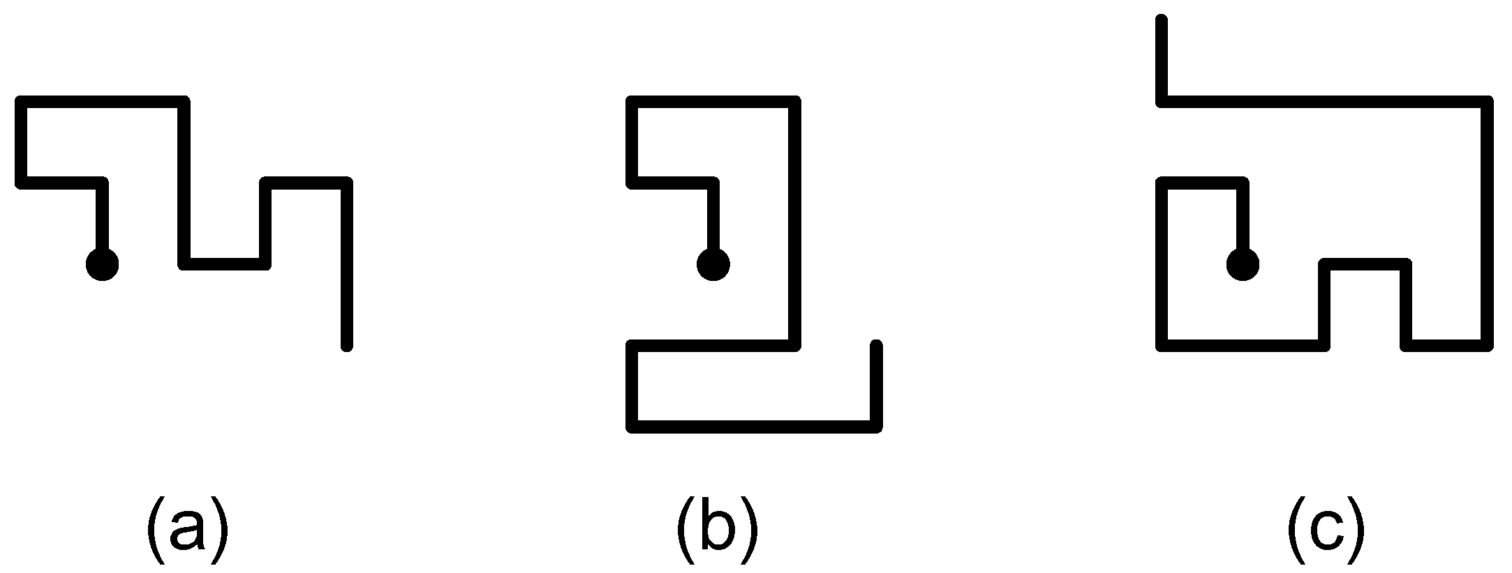
We show examples of the three types of prudent walks in Figure 1.
Figure 1.
Examples of the three types of prudent walks, (a) type 1, (b) type 2 and (c) prudent. The origin is shown as a solid ball.
Figure 1.
Examples of the three types of prudent walks, (a) type 1, (b) type 2 and (c) prudent. The origin is shown as a solid ball.
2. Type 1 prudent walks
For prudent walks of the first type, Duchi obtained the generating function by use of the kernel method, and also found a grammar for such walks. The generating function is
It has been given in a slightly different form in [2]. It is straightforward to show that the dominant singularity is a simple pole located at the real positive zero of the polynomial 1 − 2x − 2x2 + 2x3, notably x = xc = 0.4030317168 . . . . Thus the critical exponent γ = 1, and the asymptotic form of the coefficients is
for any . It is straightforward to show from (1) that
An alternative form of (1), expressed in terms of q(x), will turn out to be useful. Define
Then Bousquet-Mélou [2] showed that (1) can be written
In this form the denominator clearly has three poles. The closest to the origin corresponds to the factor 2x − q(x).
The generating function also satisfies the second order linear ordinary differential equation (ODE), with f (x) = C(1)(x)
where
P2(x)f″(x) + P1(x)f′(x) + P0f(x) = 0,
The algebraic solution is much simpler, while the ODE clearly shows the D-finite structure—not that this demonstration is strictly necessary, as any algebraic function is D-finite.
There is a second, square-root singularity just a little farther along, at . . . . We could take this term into account and write the asymptotic form of the coefficients more precisely as
The second term decays exponentially compared to the dominant term, but is included as it is still very significant for small values of n, since xc/x* is not much less than 1.
For self-avoiding walks the generating function is known, numerically, to have a singularity at x = xSAW ≈ 0.3790522 . . . , some 6% lower than the corresponding value for prudent walks of the first type. The model of prudent walks thus has a singularity numerically closer to that of SAW than any other simple model of which we are aware. Alternatively expressed, while prudent walks are exponentially rare among SAW, other simpler models are exponentially rarer than prudent walks. However the size of such walks is less interesting. Bousquet-Mélou [2] has shown that if (xn, yn) denotes the coordinates of the end-point of an n-step walk starting at the origin,
where
so that ν = 1, where is the fractal dimension of the walk. For self-avoiding walks it is known (though not proved), that .
𝔼(xn + yn) ∼ κn
3. Type 2 prudent walks
Duchi also gave a solution for prudent walks of the second type, which we discovered did not agree with our enumerations, based on the definition of prudent walks of the second type. Duchi [4] subsequently confirmed a subtle error in her calculations, due to the cancellation of two factors in her derivation. Our numerical analysis, based on a series of more than 300 terms in length, gave extremely strong evidence of identical dominant asymptotic behaviour to that of prudent walks of the first type. That is to say, the generating function has a simple pole singularity located at . . . . There was also evidence for several further singularities on the real axis. The asymptotic form of the coefficients is therefore
where ρ < x′ and x′ is the location of the first singularity on the positive real axis beyond xc. We estimated numerically that λ(2) ≈ 6.33. This is about 2.5 times larger than the amplitude, λ(1) of type 1 prudent walks. It seems to us remarkable, and far from obvious, that the critical point for type 2 prudent walks should be the same as for type 1 prudent walks.
This conjectured asymptotic result has recently been confirmed by Bousquet-Mélou [2], who has obtained the exact generating function, which of course contains far more information than our conjectured asymptotic behaviour.
Recalling that q(x) is defined by (2), the generating function for type 2 prudent walks is
where
and
In this case the asymptotics are much more difficult to establish. Bousquet-Mélou [2] has confirmed that the dominant singularity is precisely as for type 1 prudent walks, that is to say a simple pole located at the real positive zero of the polynomial 1 − 2x − 2x2 + 2x3, notably . . . . The factor
appearing in the denominator of (3) gives rise to an infinite sequence of poles on the real axis, lying between xc and , which are not cancelled by zeros of the numerator. This accumulation of poles is enough to prove that the generating function cannot be differentiably finite, or D-finite.
Bousquet-Mélou [2] has also shown that the average width of the bounding box of a type 2 prudent walk (this is sometimes called the caliper diameter) is
so again we find ν = 1.
We also obtained series expansions for the anisotropic version of the problem. The anisotropic generating function is defined as follows: If denotes the number of type 2 prudent SAW with m horizontal steps and n vertical steps, then the anisotropic generating function can be written
where is the (rational [12]) generating function for prudent type 2 SAW with n vertical steps. The functions Tn(x) are found to be (numerically) of the form
where P2n denotes a polynomial of degree 2n.
This simple denominator structure does not preclude a D-finite generating function, and is a hallmark of a solvable model. It is reassuring that the solution has been found. It is also likely that the functional equation given in [2] could be enhanced by distinguishing x and y steps, and thus be used to confirm this observation.
4. Prudent walks
For prudent walks, Duchi gave two coupled equations which can be iterated to give the series coefficients of prudent walks in polynomial time. Rechnitzer [7] pointed out that these equations can be combined into a single equation,
which must be iterated, and the generating function obtained by setting u = v = w = 1. A closed form solution for this problem has not been found. The variables (u, v, w) appearing above are called catalytic variables. In Bousquet-Mélou’s [2] solutions, type 1 prudent walks were formulated in terms of a functional equation with a single catalytic variable (the distance of the end-point from the north-east corner of the bounding box). Type 2 prudent walks were formulated in terms of a two catalytic variables (required to locate the end-point with respect to the north-east and south-east corners of the bounding box). For prudent walks, three such variables are required to uniquely specify the end-point.
To solve functional equations similar to (4) with only two catalytic variables is already a calculational tour de force, as can be seen from the solution of type 2 prudent walks. We don’t know how to solve such equations with three catalytic variables, but the equations can be iterated, thus producing series expansions in polynomial time. As a further check, we calculated the series expansions directly from the definition of the walks, without resort to the functional equation (this is in fact how we found the error in the initially proposed solution of type 2 prudent walks.) The enumeration is described in section 5 below.
In this way we obtained a series of more than 400 terms. These were analysed by a variety of standard methods, as detailed in [8] and once again we found that the generating function is dominated by a simple pole singularity located at x = xc = 0.4030317168 . . . . The asymptotic form of the coefficients is therefore
where we estimated numerically that λ ≈ 16.12. This is about 2.5 times larger than the amplitude, λ(2) of type 2 prudent walks. It is not clear from the functional equation, nor from any geometrical arguments we can muster that the critical point should be unchanged, nor that the critical exponent should be unchanged, and a simple pole. Indeed, it is only clear from the rather long series that we have. From a series of length 100 terms, one could not extract these results. We can get some clue as to why the series, even with 100 terms, behaves so badly. We see that the generating function for type 2 prudent walks has an infinite number of poles in the interval (xc, ). It is reasonable to expect, and this is confirmed by our numerical studies, that something similar occurs for prudent walks. Then the asymptotic behaviour of the coefficients could be written more precisely as
where ρ < x′ and x′ is the first pole on the real axis satisfying x′ > xc. This last term decays exponentially compared to the dominant term. Even though this is an exponentially decaying term, for values of n even as high as 100, it can still have a significant effect on the magnitude of the series coefficients, just as we saw was the case for type 2 prudent walks. Enumerations of the size of prudent walks also allows us to confidently conjecture that ν = 1, just as for type 1 and type 2 prudent walks.
Note that for both type 1 and type 2 prudent walks the location of the dominant singularity comes from the solution of the equation
where q(x) is defined in (2). The observed asymptotic behaviour then provides a strong hint that the (unknown) solution for prudent walks will also involve the function q(x), in such a way that the critical behaviour is given by a pole at the solution of q(x) = 2x.
q(x) = 2x,
As for type 2 prudent walks, we also obtained series expansions for the anisotropic version of this problem, which allows us to conjecture that the generating function is not D-finite. The anisotropic generating function is written
where is the (rational [12]) generating function for prudent SAW with n vertical steps.
We find the following for the denominators Nn(x).
N1(x) = (1 − x)
N2(x) = (1 − x)2
N3(x) = (1 − x)3(1 + x)
N4(x) = (1 − x)4(1 + x)2
N5(x) = (1 − x)5(1 + x)3(1 + x + x2)
N6(x) = (1 − x)6(1 + x)4(1 + x + x2)2
N7(x) = (1 − x)7(1 + x)5(1 + x + x2)3(1 + x2)
N8(x) = (1 − x)8(1 + x)6(1 + x + x2)4(1 + x2)2
N9(x) = (1 − x)9(1 + x)7(1 + x + x2)5(1 + x2)3(1 + x + x2 + x3 + x4)
If this pattern persists, the generating function cannot be D-finite, as the pattern of cyclotomic polynomials of increasing degree suggests a build-up of zeros on the unit circle in the complex x plane, and such an accumulation is incompatible with D-finite functions.
5. Computer enumeration
We use a transfer-matrix algorithm to count the number of prudent SAWs. Given a walk that is a prefix of a prudent SAW, we can determine in how many ways that walk can be extended to form a prudent SAW with only a small amount of information about the walk. This information is called a configuration. All SAWs of a given length correspond to one of a finite number of these configurations. Our algorithm progresses by computing how many walks exist of each possible configuration up to a given size of walk n. The information that must be stored in a configuration depends on which of the objects (type 1, type 2 or full prudent walks) we are counting.
Consider prudent walks. In a partial walk of some number of steps, there will be a minimal bounding box of the walk. It is easy to show that the end of the walk will be on an edge of this box. The next step must either move away from the box, making it larger, or along the current edge, which is possible only if no sites of the walk lie in that direction.
The information in the configurations we use for these walks is the dimensions of the bounding box, which edge the end of the walk is on, the location of the end of the walk on that edge, and an integer representing whether there are sites of the walk along the edge to the left of the end, to the right of the end, or neither. (Both is not possible.)
When we move from an edge to a corner of the bounding box, we consider the end of the walk to have moved to the other edge only if that edge has been moved outward by the step.
Without loss of generality, we can assume that we are always on the top edge of the bounding box, since by symmetry direction is not important for prudent walks. We can also assume that the end of the walk is not farther from the left edge than from the right edge, since the number of ways a walk can be completed is invariant under reflection.
For a given configuration, there are three possible steps a walk with that configuration can take:
- A step outward, away from the current edge;
- A step to the left along the current edge, if there are no walk sites in that direction;
- A step to the right along the current edge, if there are no walk sites in that direction.
The transfer-matrix algorithm then proceeds by simulating one walk step at a time, keeping a list of the possible configurations and the number of walks that produce that configuration. The algorithm steps through the list, and for each configuration, finds the configurations that can be generated by adding one step, and adds the number of walks with the current configuration to the number of walks with each of those new configurations. The number of walks of each length is the sum of the number of walks for each of the configurations in the list for that length.
In prudent walks of types 1 and 2, we cannot ignore the direction of the current edge in our configuration, since some steps may be disallowed depending on their direction. So we cannot assume that the endpoint is on the top edge, or arbitrarily reflect the configuration, since rotations and reflections of a configuration are not equivalent. However, for type 1 walks we can reflect about the southwest-to-northeast axis; and for type 2 walks we can reflect about the east-west axis.
Apart from precisely what information is required in the configuration, the test for which steps are valid from a given configuration, and which configurations should be accumulated to give the result, the algorithm to enumerate each of the three objects is identical. So we produced one program to solve all of these problems. The lists are stored in hash tables for efficiency. The number of walks for each configuration and the total number of walks are computed modulo a large number close to the computer’s word size. The computation is repeated for several such numbers and the final result is calculated by reconstruction using the Chinese Remainder Theorem. This is more efficient than performing the whole calculation using numbers larger than the computer’s word size.
The series for prudent walks can be obtained from www.ms.unimelb.edu.au/˜ tonyg. For type 1 and type 2 prudent walks they can be obtained by expanding the exact solution.
6. Conclusion
We have studied type 1, type 2 and full prudent walks. For the first two we have little to add to pre-exisitng work [2, 3], apart from some minor additional numerical work, but for the full problem we have four strong conjectures. These are (i) the exact value of the critical point, (ii) the exact value of the critical exponent γ, (iii) the exact value of the critical exponent ν, and (iv) the conjecture that the generating function is not D-finite. Bousquet-Mélou [2] has also considered prudent walks on the triangular lattice. In that case the bounding “box” is a triangle, and the relevant functional equation has only two catalytic variables, and so she can solve it. She finds similar behaviour to that observed for square-lattice prudent walks, a simple pole in the walk generating function, located at a point given by the solution of a cubic polynomial, and exponent ν = 1. She also proves that the generating function is not D-finite.
It still seems to us remarkable that type 1, type 2 and prudent walks should have identical critical behaviour, differing only in their critical amplitude. One might hope for a simple argument to, at least, prove that the radii of convergence are the same, but such an argument has eluded us.
The critical amplitude increases by a factor of about 2.5 in going from type 1 to type 2 prudent walks, and again by a similar (but not identical) factor in going from type 2 to prudent walks. As this factor, is very close to 1/xc ≈ 2.481 . . . it appears that, loosely speaking, asymptotically type 2 walks of n steps behave as type 1 walks of n + 1 steps and prudent walks of n − 1 steps.
The three generating functions are also of interest as a test-bed for series analysis techniques. The type 1 generating function has two singularities on the positive real axis quite close together. The type 2 generating function has an infinite sequence of poles on the real axis, all quite close to the physical singularity, and we conjecture similar behaviour for the prudent walk generating function. As a consequence, rather long series are required before the asymptotic regime is reached.
In subsequent work we will report on prudent self-avoiding polygons, and a three-dimensional version of prudent walks.
Acknowledgments
We would like to thank Simone Rinaldi and Enrica Duchi for introducing us to this problem, and Mireille Bousquet-Mélou for several enlightening discussions, and access to her results prior to publication. This work was completed while AJG enjoyed the hospitality of the Isaac Newton Institute for Mathematical Sciences, which he gratefully acknowledges, as well as financial support from the Australian Research Council.
References
- Bousquet-Mélou, M. A method for the enumeration of various classes of column-convex polygons. Disc. Math. 1996, 154, 1–25. [Google Scholar] [CrossRef]
- Bousquet-Meélou, M. Families of prudent self-avoiding walks. 2008; [arXiv: math.CO 0804.4843v1]. [Google Scholar]
- Duchi, E. On some classes of prudent walks. In Proceedings of the FPSAC’05, Taormina, Italy, 2005.
- Duchi, E. Personal communication, 2006.
- Preéa, P. Exterior self-avoiding walks on the square lattice. 1997; (manuscript). [Google Scholar]
- Turban, L.; Debierre, J.-M. Self-directed walk: a Monte Carlo study in two dimensions. J. Phys. A 1987, 20, 679–686. [Google Scholar] [CrossRef]
- Rechnitzer, A. Personal communication. 2006. [Google Scholar]
- Guttmann, A. J. Asymptotic analysis of coefficients. In Phase Transitions and Critical Phenomena; Lebowitz, J., Domb, C., Eds.; Academic Press: London, 1989; 234 p. [Google Scholar]
- Guttmann, A. J.; Enting, I. G. On the solvability of some statistical mechanical systems. Phys. Rev. Letters. 1996, 76, 344–347. [Google Scholar] [CrossRef]
- Rechnitzer, A. Haruspicy and anisotropic generating functions. Advances in Applied Mathematics 2003, 30, 228–257. [Google Scholar] [CrossRef]
- Stanley, R. P. Differentiably finite power series. European J. Combin 1980, 1, 175–188. [Google Scholar] [CrossRef]
- Stanley, R. P. Enumerative Combinatorics; Cambridge University Press: Cambridge, 1999; Vol. 2. [Google Scholar]
© 2008 by the authors licensee Molecular Diversity Preservation International, Basel, Switzerland. This article is an open-access article distributed under the terms and conditions of the Creative Commons Attribution license ( http://creativecommons.org/licenses/by/3.0/).
Share and Cite
MDPI and ACS Style
Dethridge, J.C.; Guttmann, A.J. Prudent Self-Avoiding Walks. Entropy 2008, 10, 309-318. https://doi.org/10.3390/e10030309
AMA Style
Dethridge JC, Guttmann AJ. Prudent Self-Avoiding Walks. Entropy. 2008; 10(3):309-318. https://doi.org/10.3390/e10030309
Chicago/Turabian StyleDethridge, John C., and Anthony J. Guttmann. 2008. "Prudent Self-Avoiding Walks" Entropy 10, no. 3: 309-318. https://doi.org/10.3390/e10030309