Improvement of Energy Conversion/Utilization by Exergy Analysis: Selected Cases for Non-Reactive and Reactive Systems

Abstract

Exergy analysis is a powerful and systematic tool for the improvement of energy systems, with many possible applications in both conversion and utilization of energy. Here we present selected applications, with a special attention to renewable energy systems (solar), covering both design and operation/control. After these applications to non-reactive systems, potential ways of reducing the large irreversibilities connected to reactive systems (combustion) are considered, with special reference to chemically-recuperated gas turbine cycles and topping high-temperature fuel cells.

1. Introduction

Exergy analysis is a recognized method for the analysis and optimization of energy systems [1,2,3,4,5,6]. It is widely documented both in energy conversion (with special reference to thermal or thermo-chemical options) and energy utilization (from cooling to industrial heat/process applications). Without pretending to be exhaustive, the present paper presents some applications ranging from design to control, applied to non-reactive and reactive energy systems.

2. Non-Reactive Energy Systems

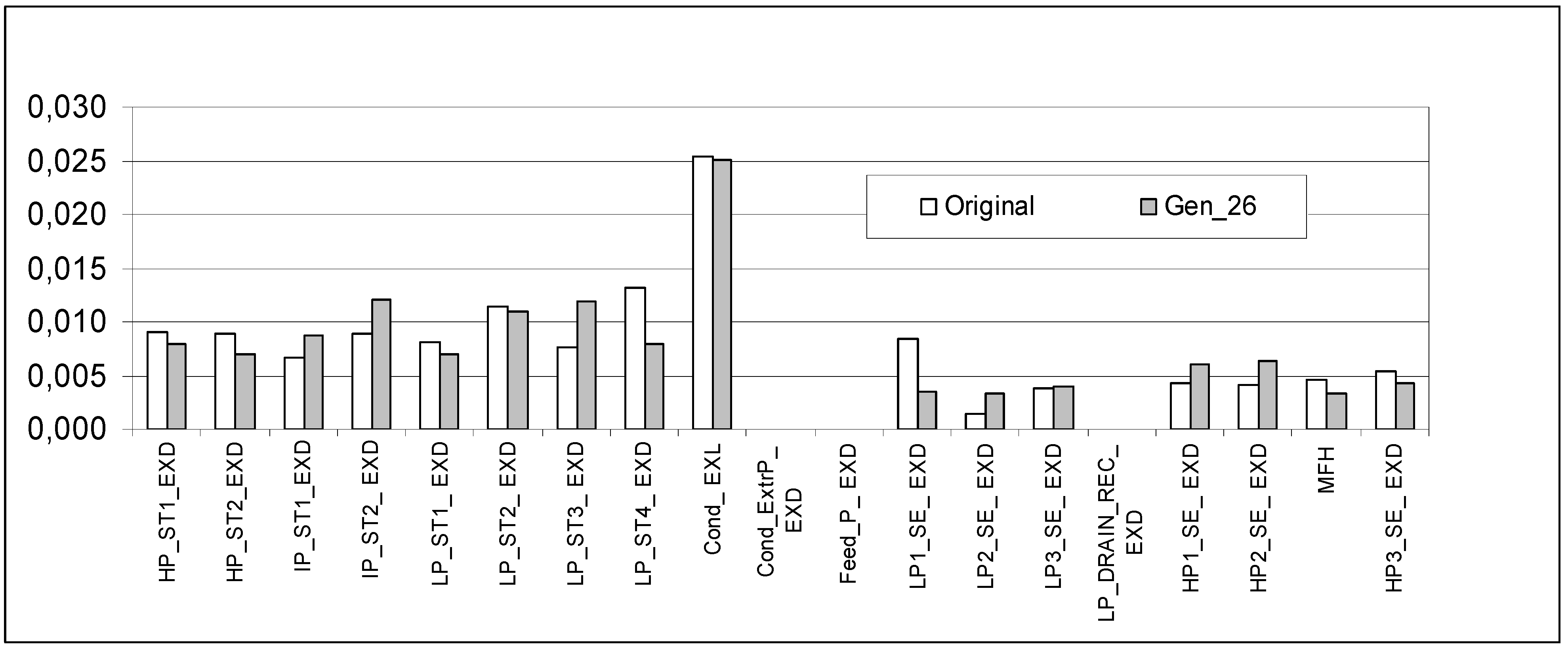
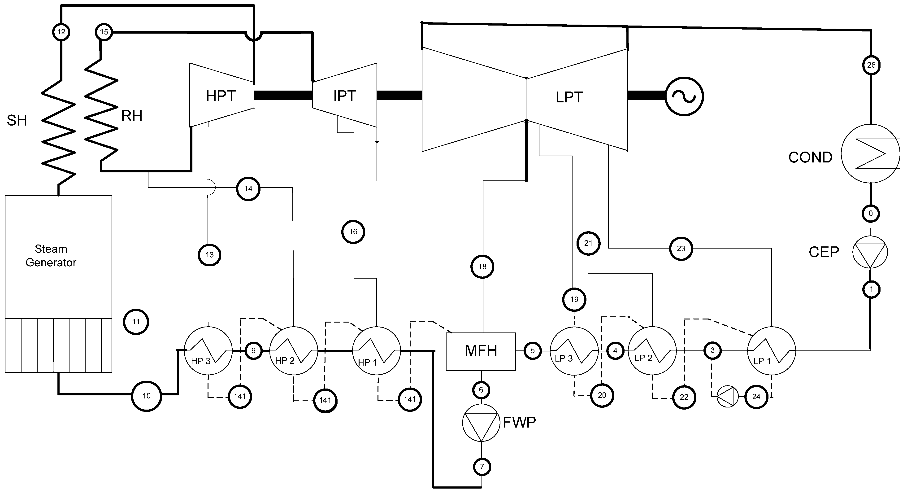
2.1. Case 1—332 MWe Steam Power Plant (Energy Conversion; Design/Optimization)

The first test case is a reference 332 MWe Power plant (Figure 1). Its layout has been slightly simplified with respect to a true power plant, basically neglecting shaft seal steam recovery. The steam cycle has 3 high-pressure and 3 low-pressure surface heat exchangers (HP_ST1-3; LP_ST1-3); a Mixing Feedwater Heater (MFH, serving also as de-aerator for removal of non-consensable gases) separates the feedwater line in the high and low-pressure sections. The main data are collected in Table 1. The system is simulated using EES32 [7]; from the base case (ENEL power plant data), a genetic algorithm optimization was run in order to determine the set of the seven extraction pressures (Table 1) that optimize the plant thermal efficiency. A small margin for improvement was found, with some adjustments of extraction pressures that should not impair the assumed values of the steam turbine efficiencies. Figure 2 collects the results of the 19 exergy destructions and losses calculated for the steam power plant. The inlet exergy is assumed at steam cycle level, that is, the exergy difference between points (12)–(10) for the main flow stream and points (15)–(14) for the RH flow stream; exergy destructions/losses were calculated according to standard practice [1,2,5]. It is interesting to notice that the optimization process leads to the reduction of some exergy destructions, and to the increase of some others. The optimized set of extractions sees a notably lower value of the LP1 pressure, and an increase in the HP extraction pressures; indirectly, varying the mass flow rates of the extractions causes a variation of the steam turbine exergy destructions.

Figure 1. Schematic of 332 MWe Power Plant.

Figure 1. Schematic of 332 MWe Power Plant.

2.2. Case 2—Solar Thermal Steam Power Plant (Energy Conversion; Standard/Optimum Control)

The second test case is a solar thermal energy conversion plant, whose schematic is shown in Figure 3. The arrangement corresponds to common practice encountered in large solar thermal fields, such as is documented in references [8,9,10]. The solar collector field is usually arranged as a solar farm of parabolic-trough collectors, which are heating a high-temperature heat transfer fluid. The heat transfer fluid is maintained in liquid conditions even at very high temperatures (up to 400 °C for silicon oils such as Therminol VP-1 [13]); it is circulated through a primary circuit to the steam generator, where it generates steam from liquid water at inlet (secondary circuit). Steam is then expanded in a traditional superheated steam cycle, usually including a Mixing Feed-water Heater (MFH) for an effective removal of non-condensable gases. This is the typical layout for reference power sizes larger than 1 MW_e, while for lower power ratings Rankine Organic Cycles (ROC) [8,13,18] are gaining increasing popularity. The discussion in the following is aimed at control applications, and it applies both to steam and ROC power cycles.

Figure 2. Relative exergy destructions/losses for the 332 MWe Power Plant.

Figure 2. Relative exergy destructions/losses for the 332 MWe Power Plant.

Table 1. Steam Cycle parameters (bold = calculated).

Variable	Base Case	Optimized
ηHPT	0,88	0,88
ηIPT	0,89	0,89
ηLPT	0,90	0,90
TSH = TRH °C	538	538
pCond bar	0,05	0,05
pSH bar	170	170
p13 bar	78,3	88,03
p14 bar	37,75	49,91
p16 bar	16,94	19,02
p18 bar	7,24	6,454
p19 bar	2,6	2,661
p21 bar	0,76	0,7295
p23 bar	0,29	0,1481
η	0,4687	0,4710
ηx	0,869	0,871
Generation	1	26

Table 1. Steam Cycle parameters (bold = calculated).

Variable	Base Case	Optimized
ηHPT	0,88	0,88
ηIPT	0,89	0,89
ηLPT	0,90	0,90
TSH = TRH °C	538	538
pCond bar	0,05	0,05
pSH bar	170	170
p13 bar	78,3	88,03
p14 bar	37,75	49,91
p16 bar	16,94	19,02
p18 bar	7,24	6,454
p19 bar	2,6	2,661
p21 bar	0,76	0,7295
p23 bar	0,29	0,1481
η	0,4687	0,4710
ηx	0,869	0,871
Generation	1	26

Figure 3. Solar Thermal Energy conversion plant.

Figure 3. Solar Thermal Energy conversion plant.

Control of solar thermal power plants has not up to now received much attention from the scientific community. As these power plants are still in the start-up phase, the first goal is to demonstrate that they are efficient and reliable: in order to do that, and considering the variability of the solar source over time, the steam plant is usually operated under fixed thermodynamic conditions (pressure and temperature). A typical current control law [10,15] uses a fixed set-point temperature at collector outlet, T_fo; consequently, the temperature of superheated steam T₆ is also fixed; the flow rates in the primary and secondary system circuits are adjusted according to the availability of solar radiation. Seasonal adjustments to T_fo and T₆ are usually necessary. This operation law has some technical sense, as it minimizes thermal expansion problems - a common critical issue in solar farms using a large number of parabolic-trough collectors. However, a strong reduction of the flow rate through the primary and secondary loops results when the solar radiation is very low, at morning or in the evening. Under such conditions the collectors are driven to stagnation conditions, that is, operation with a very high heat loss to the environment, and efficiency close to zero [11]. In order to minimize such problems, storage devices are added to the circuit, or external heating integration is used (e.g., with an auxiliary burner using a conventional fuel). In some cases, silicon oil is substituted with molten salts [14], which must be maintained under liquid conditions even at night: this is obtained using heat from a large combined-cycle gas turbine exhaust.

The authors believe that when trying to efficiently use natural energy resources that are subject to large and/or un-expectable variations in time, such as solar, wind or wave energy, the energy conversion plant should be operated following as close as possible the conditions dictated by nature. In the case of solar energy, this means that when radiation is low we should accept operation of the solar thermal conversion plant not only with reduced flow rate, but also with adjusted (reduced) parameters (steam pressure and temperature). Exergy is a very useful tool in this case [13,16,17]. The data presented in Figure 4 was calculated for a typical commercial parabolic trough collector. It demonstrates that the collector outlet temperature (for fixed inlet temperature conditions) should be chosen in order to maximize the exergy efficiency of the collector. The maximum exergy condition (ME) is strongly affected by solar radiation. From the curves shown in Figure 4, the following conclusions can be drawn:

-

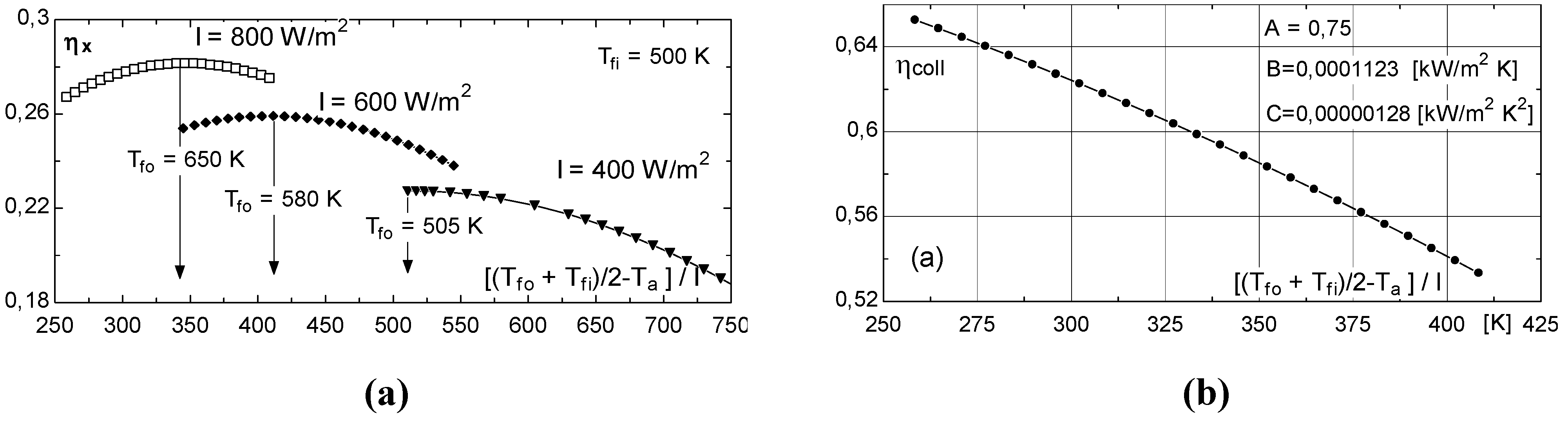
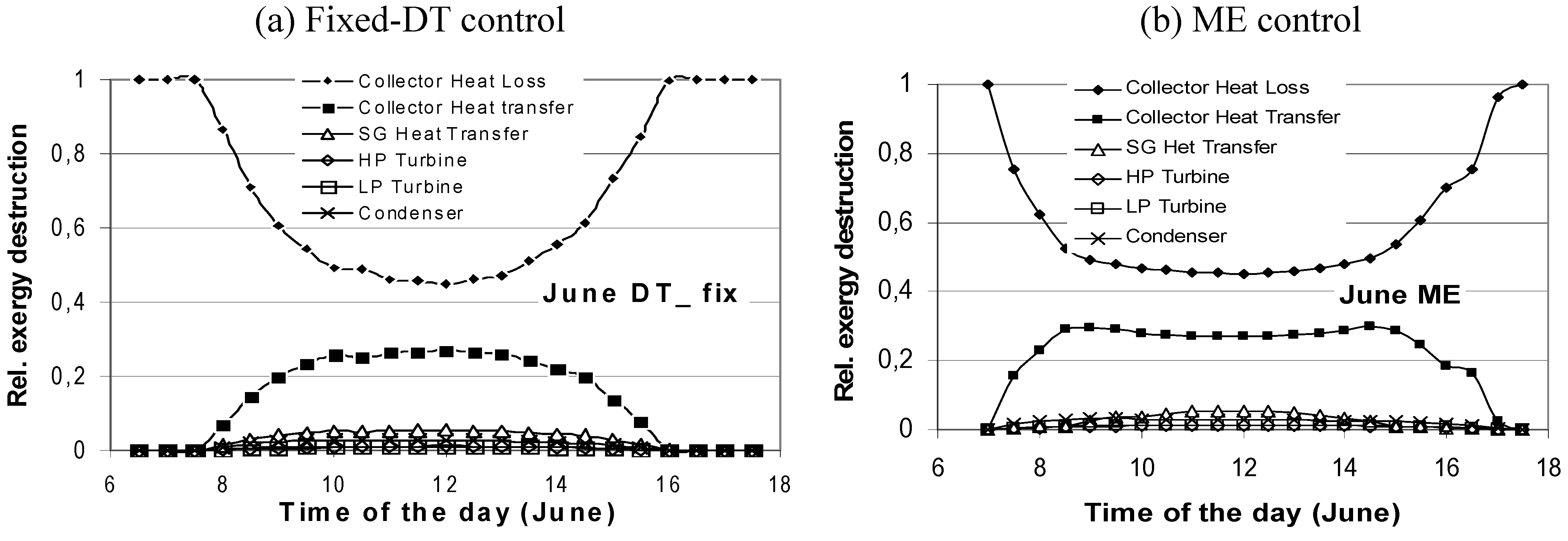
In order to have low thermal losses and transfer most of the heat to the fluid, the solar collector should be operated at a high thermal efficiency, with a low average absorber temperature (T_fo + T_fi)/2. The collector transfers large quantities of heat to the fluid, but it is low-quality heat.

-

If the average absorber temperature is raised, the collector transfers less heat to the fluid (but with a higher quality); the heat loss to the environment is increased. If I is low or T_fo is raised too much, the collector reaches shut-off conditions (no useful energy output, zero efficiency)

-

Between these two conditions (which depend on T_a and I, as well as on T_fo), a condition of maximum exergy output (referring to the collector) must exist.

Referring to the plant schematic in Figure 3, the collector inlet temperature T_fi is determined by two conditions:

-

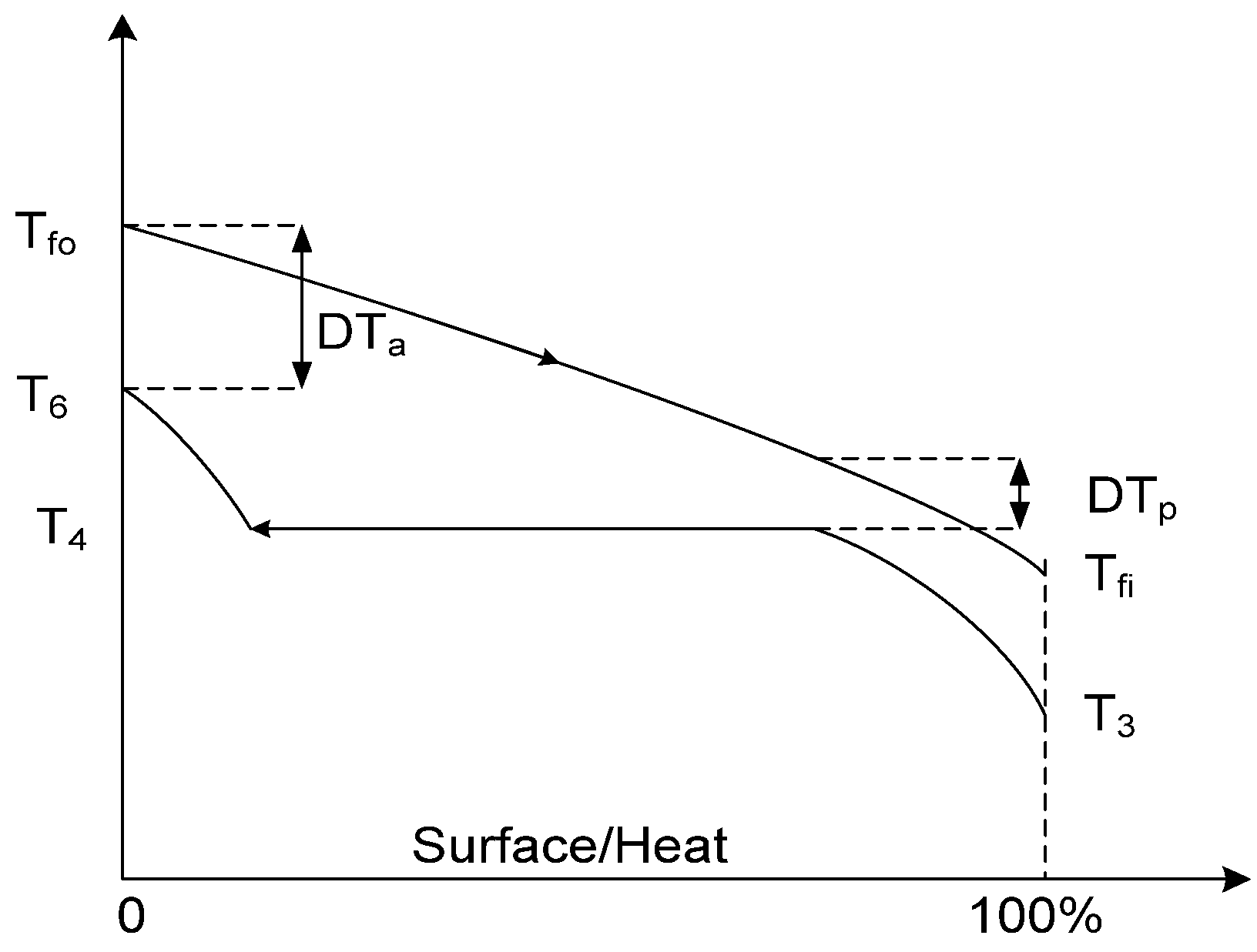
The pinch temperature difference in the steam generator.

-

The operating pressure of the MFH, which in turn determines the saturated liquid conditions at its outlet.

Figure 4. (a) Exergy efficiency of a parabolic trough solar collector under different radiation conditions. (b) Thermal efficiency of the collector

Figure 4. (a) Exergy efficiency of a parabolic trough solar collector under different radiation conditions. (b) Thermal efficiency of the collector

Looking at the steam generator temperature/surface diagram, it makes sense that, when radiation is low and it is not possible to reach the design value of the collector outlet temperature T_fo, the plant operator should accept to operate the steam circuit with a lower pressure (and consequently a lower T₄), and a lower superheated steam temperature T₆ (e.g., maintaining the same values of the approach and pinch temperature differences, respectively DT_a and DT_p). It is true that the steam turbine would operate under off-design; however, a reduced mass (and volume) flow rate would result also if the plant were controlled with fixed set-point temperatures (T_fo and T₆), so anyway off-design operation is unavoidable (without a heat storage for short time periods, or external heat integration for longer periods).

In Rankine Organic Cycles [13,18], the turbine exit conditions are usually in the super-heated state, and a Regenerative Heat Exchanger (RHE) pre-heating the liquid before entry to the steam generator must be added. The effectiveness of the RHE and the condenser pressure substitute the MFH condition (steam case).

The maximum exergy operating conditions (shown graphically in Figure 4) can be determined by recursive analytical solution [16] only when the thermal efficiency curve of the collector (Figure 4b) is linearized. However, it is relatively simple to develop a numerical procedure, starting from a guess value (for example, obtained by linearization of the efficiency curve, such as in [16]), and searching directly for the maximum exergy condition. In the present case a chord iterative method is applied. A typical result is shown for a typical day in June in Figure 6; fixed set-point control (Figure 6a) is compared to ME control (Figure 6b). The value of the fixed DT was chosen as that maximizing efficiency at noon. It is clear that ME control causes a remarkable decrease of the collector exergy loss (heat released to the environment), at the expense of a larger collector heat transfer exergy destruction. The result is a higher overall efficiency of the whole energy conversion plant (Figure 7).

Figure 5. Pinch diagram of the steam generator.

Figure 5. Pinch diagram of the steam generator.

Figure 6. Solar thermal power plant exergy destructions/losses

Figure 6. Solar thermal power plant exergy destructions/losses

Figure 7. Solar thermal power plant efficiency (a) Fixed-DT control (b) ME control.

Figure 7. Solar thermal power plant efficiency (a) Fixed-DT control (b) ME control.

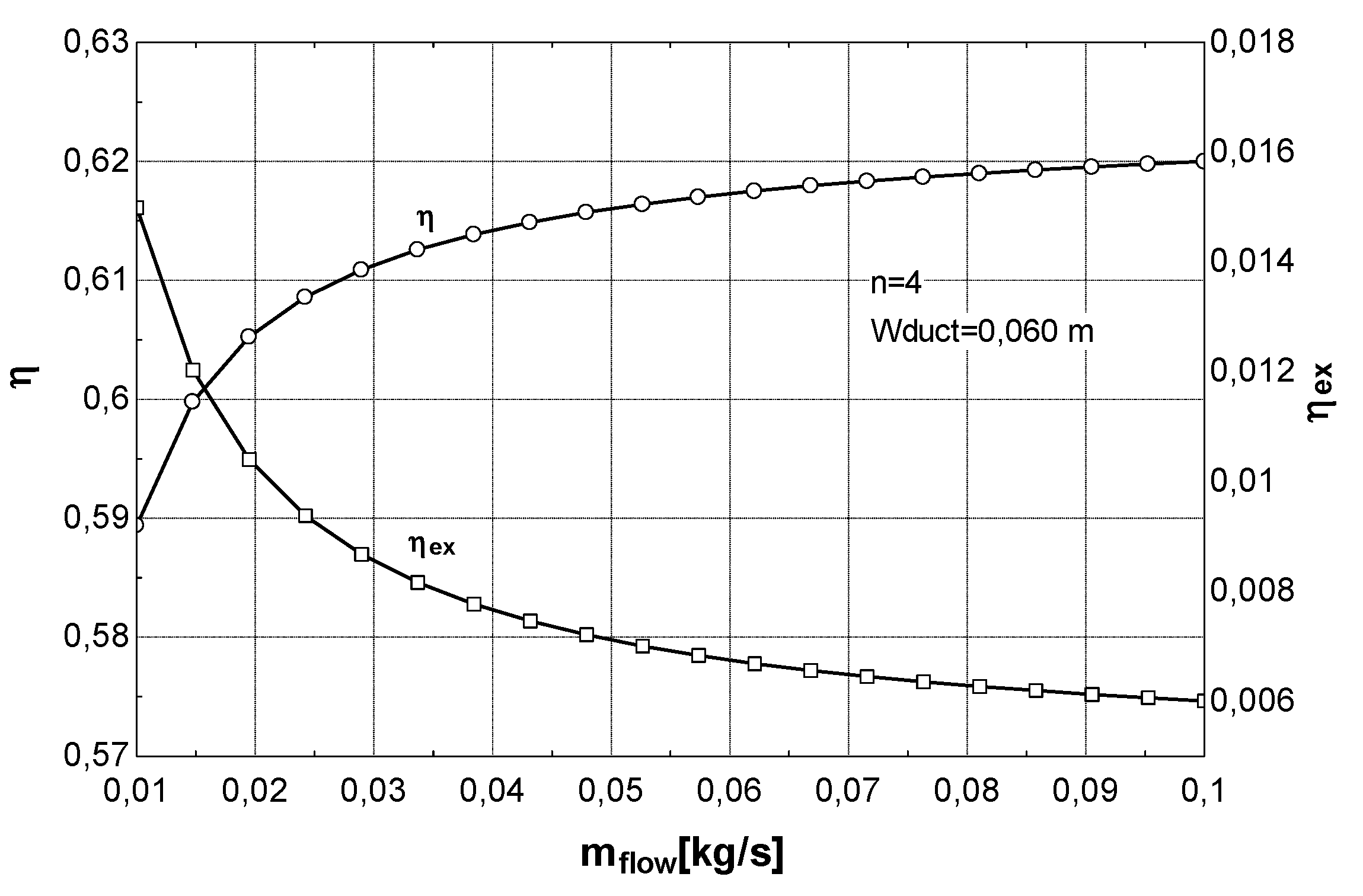
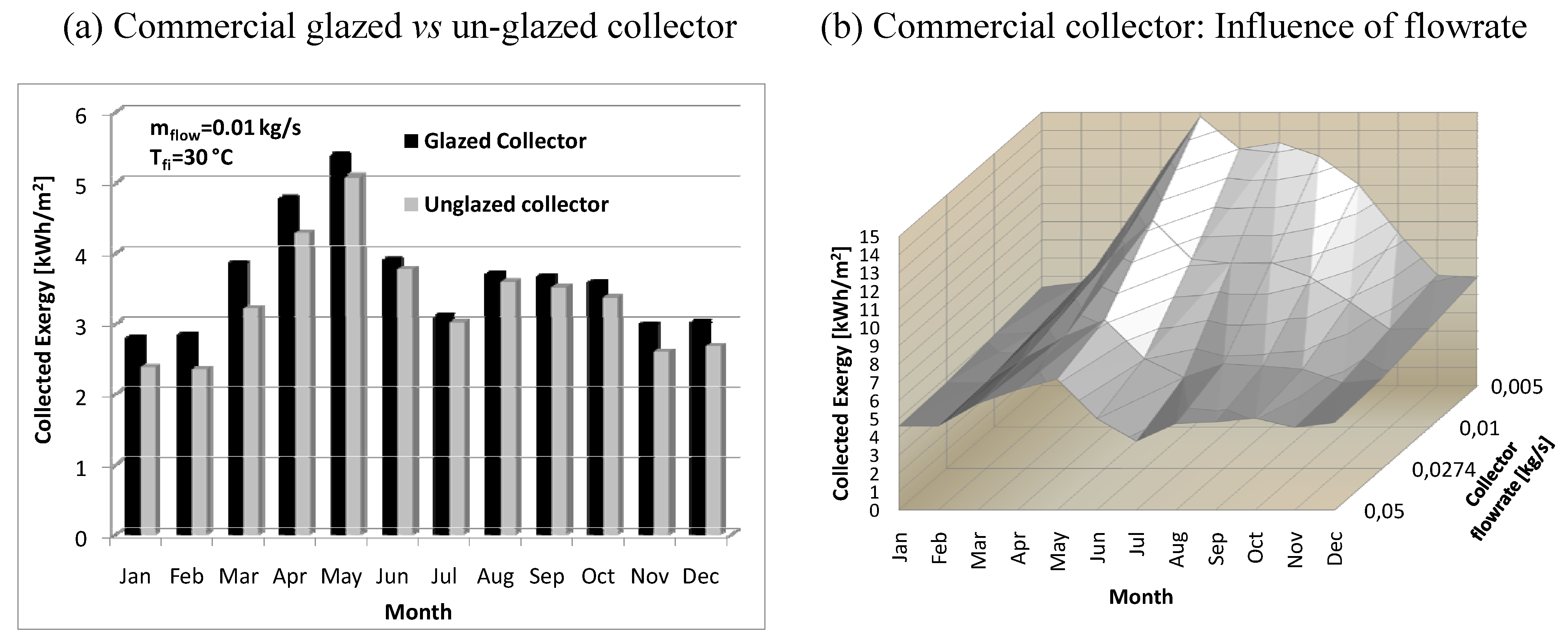
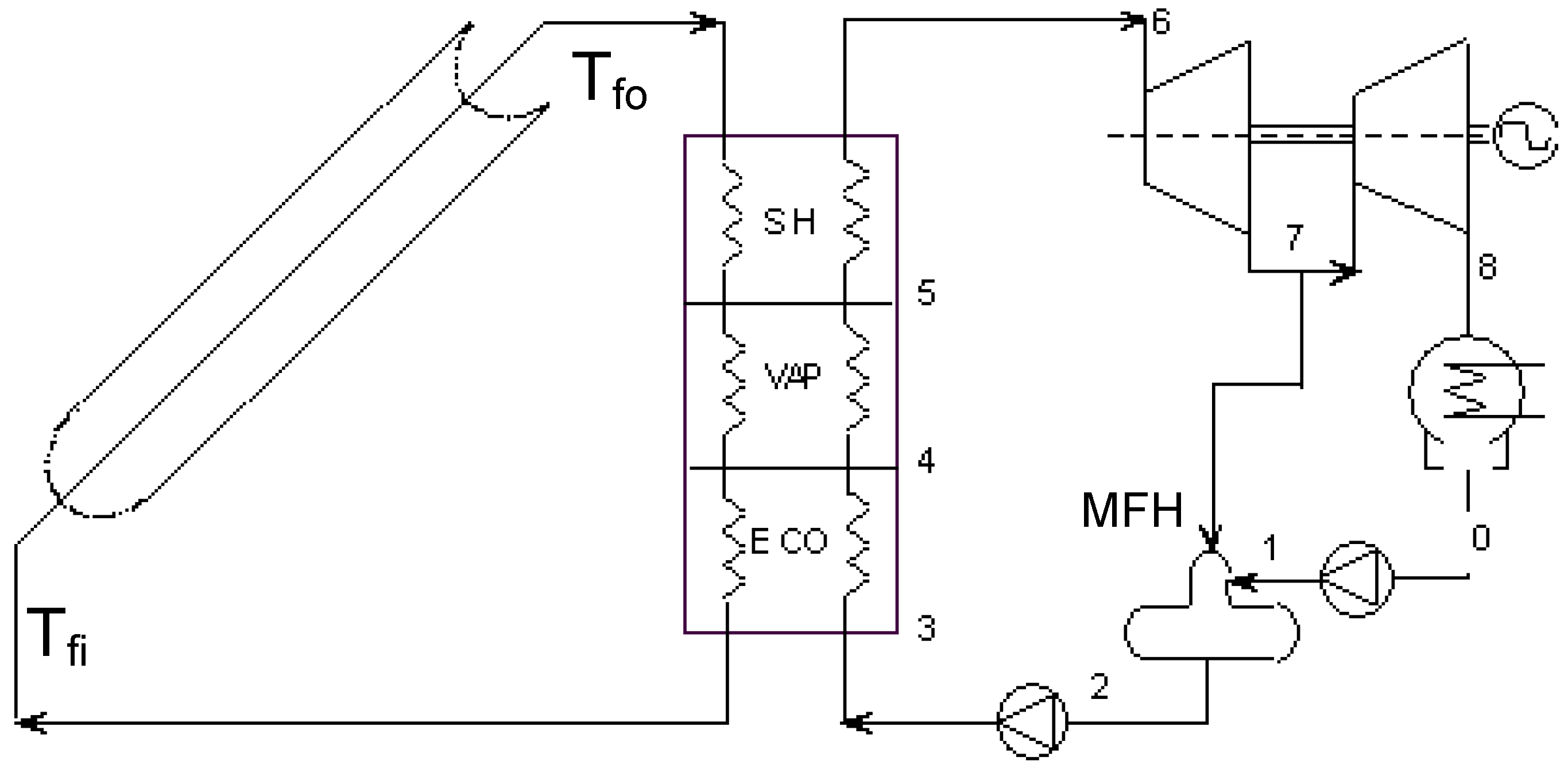
2.3. Case 3—Solar Collector Design (Thermal Utilization/Heat Transfer; Design)

Exergy analysis of solar collectors—calculation model

Solar collectors are designed to collect heat from the sun and not to convert heat into mechanical or electrical work; however, exergy analysis is interesting for three reasons:

• To determine the quality of collected heat, on the basis of its temperature, in order to somehow merge the two main performance parameters of solar collectors: efficiency and temperature rise of the fluid;
• To assess the main sources of collector exergy destructions and losses and their amount, which is closely related to temperature levels of the fluid and of the environment (the latter is the reference restricted dead state);
• To keep the exergy consumption of the pump (mechanical work) in consideration when the collector thermal performance is determined. This can be of great help in collector design because it could suggest, for example, to limit some design parameters (diameters of tube, roughness, piping layout, etc.) that lead to high values of pressure losses, and consequently, to high energy consumption of the pump.

The model for exergy analysis was added to a design tool of solar collectors, developed in EES environment [7], on the basis of a classic approach [19]. The total exergy input to the collector is the sum of two terms:

• Exergy from the sun ${\dot{\text{E}}\text{x}}_{\text{in},\text{sun}}={\text{IA}}_{\text{C}}\left(1-\frac{{\text{T}}_{\text{a}}}{{\text{T}}_{\text{sun}}}\right)$ with sun temperature defined as the 75% of the sun considered as a black body, in agreement with [20]: ${\text{T}}_{\text{sun}}=0,75\text{*}5777\left[\text{K}\right]$, T_a is the environmental reference temperature. I is the overall radiation (beam + diffused) per unit surface and A_C is the collector surface area.
• Work Exergy from the circulating pump (W_pump): $\dot{E}{x}_{in,pump}={\dot{W}}_{pump}$

The overall exergy input is then given by:

$${\dot{\text{E}}\text{x}}_{\text{in}}={\dot{\text{E}}\text{x}}_{\text{in},\text{sun}}+{\dot{\text{E}}\text{x}}_{\text{in},\text{pump}}.$$

The useful exergy extracted from the collector system is the amount related to the fluid (water) temperature increase:

$${\dot{\text{E}}\text{x}}_{\text{out}}={\dot{\text{m}}\text{c}}_{\text{p}}\left[{\text{T}}_{\text{fo}}-{\text{T}}_{\text{fi}}-{\text{T}}_{\text{a}}\text{ln}\left(\frac{{\text{T}}_{\text{fo}}}{{\text{T}}_{\text{fi}}}\right)\right]$$

Where T_fi and T_fo are inlet and outlet flow temperature, respectively, whereas c_p is the constant pressure fluid specific heat. Thus, the direct expression of collector exergy efficiency is:

$${\eta }_{ex,dir}=\frac{\dot{E}{x}_{out}}{\dot{E}{x}_{in}}$$

The indirect exergy balance can be built by the calculation of the following detailed exergy losses/destructions:

a)

Exergy loss due to incomplete absorption of the incident radiation coming from sun (a fraction is reflected by the cover—in case of glazed collectors—and the transmitted fraction is not completely absorbed by the plate). Thus, the loss is given by the difference between incident and actually absorbed radiation (S):

$${\dot{\text{E}}\text{x}}_{\text{L},\text{abs}}={\text{IA}}_{\text{C}}\left(1-\frac{{\text{T}}_{\text{a}}}{{\text{T}}_{\text{sun}}}\right)-{\text{SA}}_{\text{C}}\left(1-\frac{{\text{T}}_{\text{a}}}{{\text{T}}_{\text{sun}}}\right)$$

b)

Exergy loss due to heat dispersed to the environment:

$$\dot{E}{x}_{L,env}=U_{tot}{A}_C\left(T_p-T_a\right)\left(1-\frac{T_a}{T_p}\right)$$

Where U_tot is the overall plate—environment heat transfer coefficient and A_c the collector surface area.

c)

Exergy destruction due to the temperature difference between the sun and the absorber plate:

$${\dot{\text{E}}\text{x}}_{\text{D},\text{sun}-\text{plate}}={\text{SA}}_{\text{C}}\left(1-\frac{{\text{T}}_{\text{a}}}{{\text{T}}_{\text{sun}}}\right)-{\text{SA}}_{\text{C}}\left(1-\frac{{\text{T}}_{\text{a}}}{{\text{T}}_{\text{p}}}\right);$$

d)

Exergy destruction due to the temperature difference between the absorber plate and the fluid:

$${\dot{\text{E}}\text{x}}_{\text{D},\text{plate}-\text{fluid}}={\dot{\text{m}}\text{c}}_{\text{p}}\left({\text{T}}_{\text{fo}}-{\text{T}}_{\text{fi}}\right)\left[\left(1-\frac{{\text{T}}_{\text{a}}}{{\text{T}}_{\text{p}}}\right)-\left(1-\frac{{\text{T}}_{\text{a}}}{{\text{T}}_{\text{ml}}}\right)\right]$$

where T_ml is the log-mean inlet—outlet fluid temperature difference:

$${\text{T}}_{\text{ml}}=\frac{\left({\text{T}}_{\text{fo}}-{\text{T}}_{\text{fi}}\right)}{\text{ln}\left(\frac{{\text{T}}_{\text{fo}}}{{\text{T}}_{\text{fi}}}\right)}$$

e)

Exergy destruction due to pump work, whose only purpose is to ensure fluid motion against the piping head losses, with no additional useful effect:

$${\dot{\text{E}}\text{x}}_{\text{D},\text{pump}}={\dot{\text{W}}}_{\text{pump}}$$

f)

The collector friction loss is the sum of distributed and lumped losses; these last are due to curves, corners, etc. and are globally evaluated as $\Delta {\text{p}}_{\text{pcc}}=2\cdot 1,0\frac{{\text{v}}_{\text{flow}}^2}{2}{\mathsf{\rho }}_{\text{flow}}$. The coefficient 2 accounts for a T connection (or a 90° curve) at inlet and one at outlet. Thus, the complete expression of the friction loss—which must be compensated by direct pump work, equivalent to exergy; with a compensation for pump efficiency—is given by:

$${\dot{\text{W}}}_{\text{pump}}=\Delta {\text{p}}_{\text{tot}}\frac{{\dot{\text{m}}}_{\text{flow}}}{{\text{ρ}}_{\text{flow}}{\mathsf{\eta }}_{\text{pump}}}$$

η_pump (here assumed 0.6) is the overall pump efficiency (including fluid dynamics and electrical engine efficiency).

The final expression of the sum of the exergy losses and destructions is then:

$$\dot{E}{x}_{L-D}=\dot{E}{x}_{L,abs}+\dot{E}{x}_{L,env}+\dot{E}{x}_{D,sun-plate}+\dot{E}{x}_{D,plate-fluid}+\dot{E}{x}_{D,pump}$$

and the indirect expression of the collector exergy efficiency is:

$${\mathsf{\eta }}_{\text{ex},\text{ind}}=1-\frac{{\dot{\text{E}}\text{x}}_{\text{L}-\text{D}}}{{\dot{\text{E}}\text{x}}_{\text{in}}}$$

.

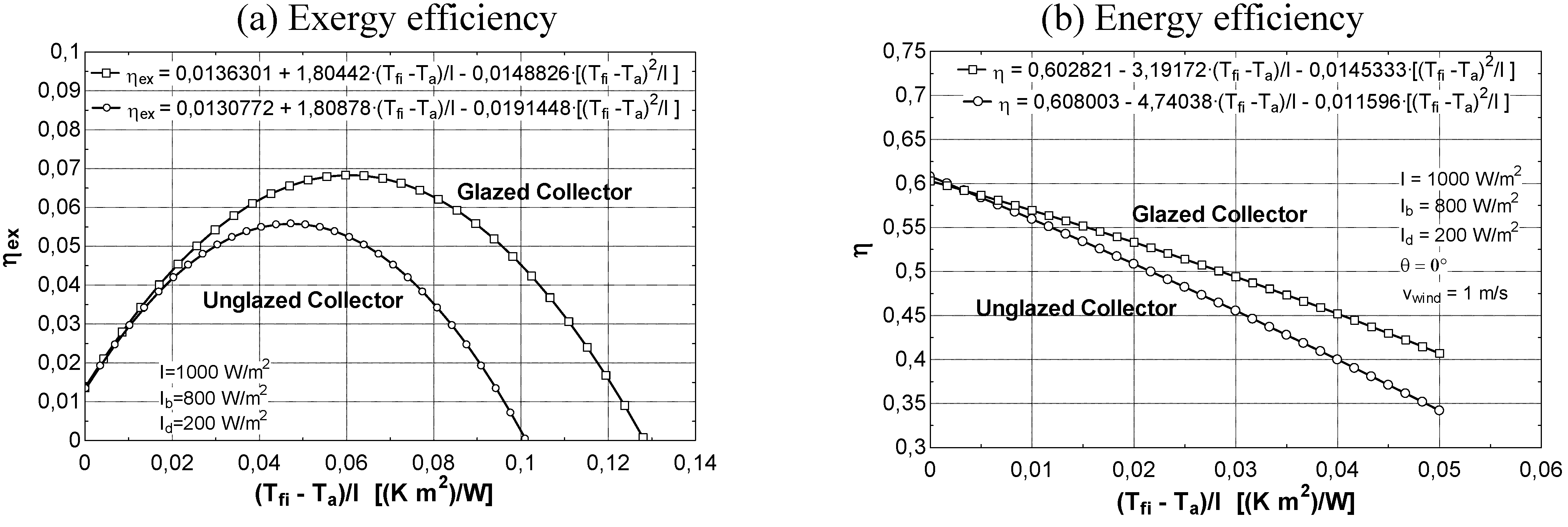
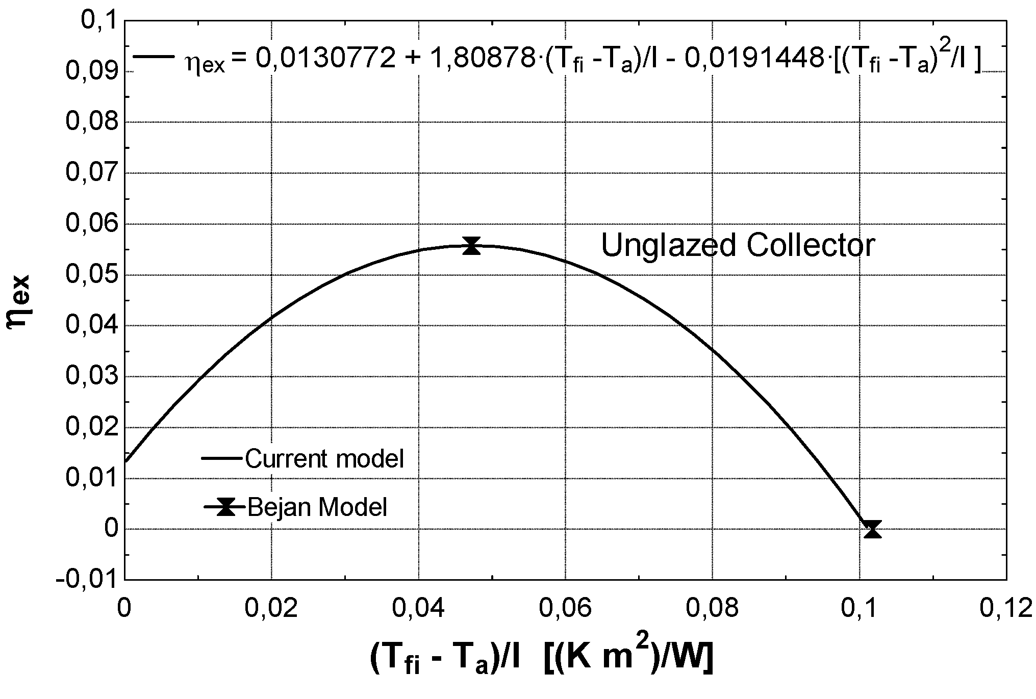
Exergy efficiency curves of solar collectors

In 1974, the National Bureau of Standards published a procedure for testing the thermal performance of solar collectors, that was later modified by ASHRAE in 1977 [11]. The procedure is aimed to determine the collector efficiency curve (η) vs. X = (T_fi – T_a)/I. It provides the fraction of solar radiation that is usefully extracted by the working fluid flowing in the collectors (Q_u) as a function of fluid inlet temperature, environmental temperature and collector design parameters:

$$\mathsf{\eta }=\frac{{\text{Q}}_{\text{u}}}{{\text{A}}_{\text{c}}\text{I}},Q_u=A_c{F}_R\left[S-U_{tot}\left(T_{fi}-T_a\right)\right]$$

where F_R is the collector heat removal factor.

In a similar manner, the exergy efficiency (η_ex) has been considered and applied to characterize a relatively innovative model of un-glazed solar collector, having interesting aesthetic features for building integration, when compared to traditional ones. It is a rectangular copper module (2.5 × 0.32 m surface) with 4 ducts (58.5 × 8.5 mm cross section) where the working fluid flows. The resulting curve is shown in Figure 8a and compared with the standard thermal efficiency characteristic of Figure 8b, under the same working and design conditions: beam (I_b) and diffuse (I_d) radiation, wind velocity (v_wind) and collector tilt (θ). Also the influence of a glass cover on the performance of the proposed collector was evaluated (glazed/un-glazed collectors).

As discussed in section 2.2 for control applications, the trend of the collector exergy efficiency curve vs. X is completely different from the ever-decreasing trend of the thermal efficiency (Figure 8). The fact that a maximum efficiency condition exists can be explained as follows:

1)

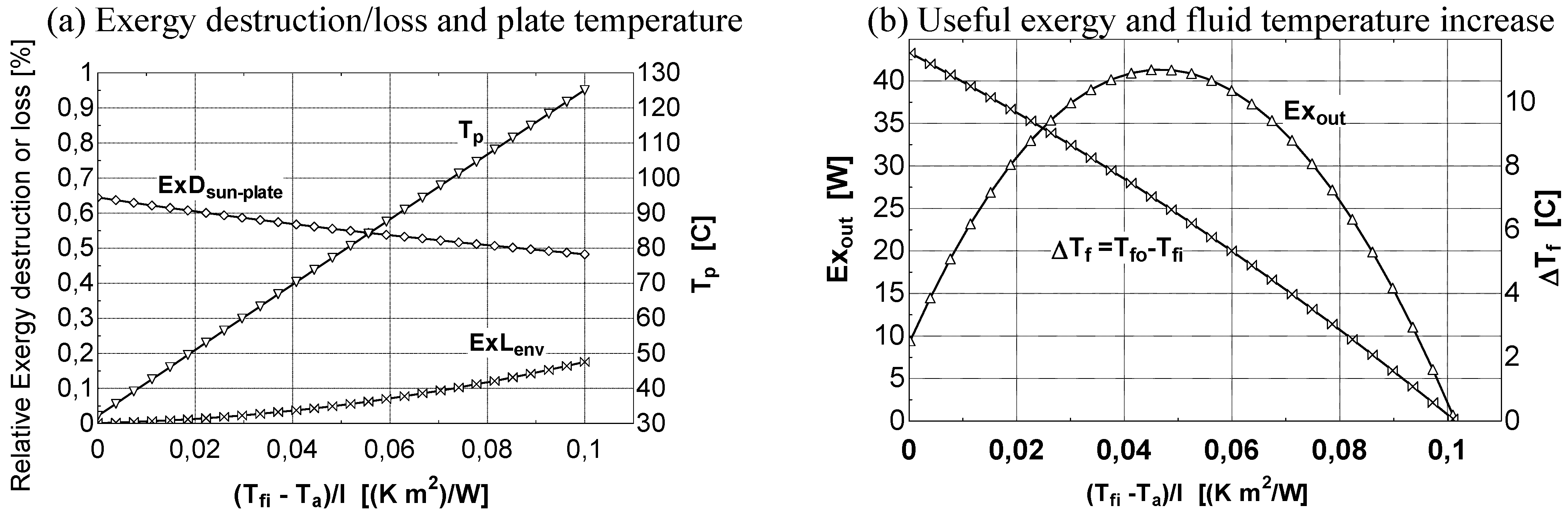
at low values of the fluid inlet temperature T_fi, the thermal efficiency reaches its maximum value (Figure 8b). On the contrary, exergy efficiency (Figure 8a) is low because the fluid and plate temperatures (very close each other) are small. A consistent fraction of the original sun radiation exergy is destroyed because of heat degradation the absorber plate temperature level, while the loss to the environment is marginal (Figure 9a).

2)

at high fluid temperatures T_fi, the exergy produced by the collector is reduced on account of large radiation/thermal losses to the environment (Figure 8a). The sun—plate exergy degradation is still large, but not dominant in defining the collector performance loss (Figure 9a).

3)

at intermediate values of temperature T_fi, the collector exergy efficiency shows an optimizing value (Figure 8a); this happens both for the un-glazed and glazed cases, corresponding to about 60–70 °C for the first one and 70–80 °C for the second one.

Differently from the energy efficiency, the exergy efficiency is not optimized at the maximum value of ΔT_f = T_fo-T_fi but at higher values of inlet temperature T_fi, corresponding in the specific case examined to a temperature rise of about 7 °C (Figure 9b)). This behavior is in agreement with the model proposed by Bejan [19], who applies a model to determine the collector inlet temperature T_fi which optimizes exergy efficiency (un-glazed collector under the same fluid inlet temperature, environmental temperature and insulation). The comparison is shown in Figure 10.

When comparing exergy and thermal efficiencies of solar collectors, another interesting point is their behavior with variable mass flow rate m_flow (Figure 11). When m_flow is increased, the thermal efficiency is also increased, because of the improved convection heat transfer coefficient between plate and flow. The opposite behavior is found for exergy efficiency, because of the effect of the increased friction losses and of the reduced temperature rise at high flowrates, which imply large exergy consumption for fluid circulation and a lower quality of the collected heat.

Figure 8. Exergy and energy characteristic curves of glazed and un-glazed solar (I = 1000 W/m², I_b = 800 W/m², I_d = 200 W/m²).

Figure 8. Exergy and energy characteristic curves of glazed and un-glazed solar (I = 1000 W/m², I_b = 800 W/m², I_d = 200 W/m²).

Figure 9. Exergy destruction/loss, useful exergy and temperature rise of solar collectors.

Figure 9. Exergy destruction/loss, useful exergy and temperature rise of solar collectors.

Figure 10. Exergy efficiency of solar collector-Comparison between current model and Bejan’s [19].

Figure 10. Exergy efficiency of solar collector-Comparison between current model and Bejan’s [19].

Figure 11. Energy (η) and exergy (η_ex) efficiency of solar collector vs. collector inlet flowrate (n = number of ducts, W_duct = duct section wide).

Figure 11. Energy (η) and exergy (η_ex) efficiency of solar collector vs. collector inlet flowrate (n = number of ducts, W_duct = duct section wide).

Finally, exergy accounting can be applied to qualify the amount of thermal energy captured by the collector covering a relatively long time period, like months or seasons. It is interesting to notice that the highest amount of exergy is collected in spring months like April and May, whereas in summer and winter worse performance levels are achieved (figure 12). This is attributable to the following reasons:

1)

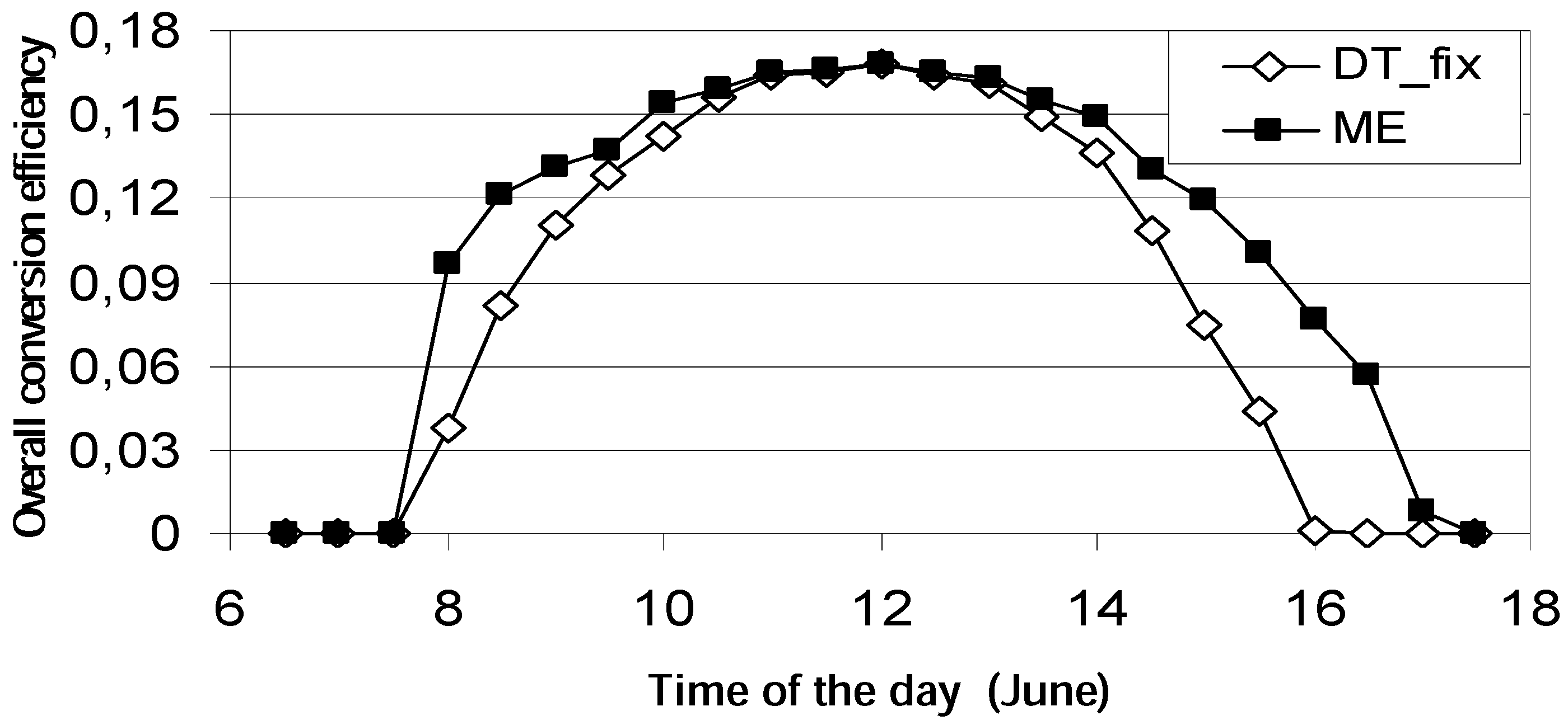
in winter the fluid temperature rise across the collector is modest, consequently the exergy collected is reduced.

2)

in summer, in spite of larger temperature rise, the higher environmental temperature (representing the reference state) is responsible for reduced exergy performance.

On the whole, the moderate levels of environmental temperatures in spring are responsible for a good exergy performance of solar collector in this season. The effect of the environmental temperature T_a is remarkable for moderate temperature rise of the working fluid (ΔT_f), whereas at high ΔT_f the influence of T_a on the exergy collected is reduced. For a fixed collector surface area, ΔT_f increases with reducing flowrate, resulting in an increase of exergy collected per square meter, as shown in Figure 12b). Moreover, in midsummer months like July, the worst performance is registered at high flowrate, whereas high levels of collected exergy can still be achieved at low flowrates in spring months like May. This suggests that the effect of increasing ΔT_f at reduced flowrate prevails over the effect of higher environmental temperatures in summer. On the whole, we can say that environmental temperature plays an appreciable effect on collected exergy when the temperature rise is relatively low, whereas it is of minor importance at relatively high ΔT_f.

From this point of view, exergy analysis applied to an existing solar collectors field can be regarded as an useful tool to adjust the flow rate according to the different energy demand and seasonal conditions: the guideline being to collect the highest possible amount of exergy. In fact, in cold time periods, when collectors heat losses to the environment are consistent, it may often be useful to reduce flow rate in order to achieve interesting values of ΔT_f, rather than working at design flow rate but with extremely modest values of ΔT_f (0–2 °C). The indication is further complicated by the addition of a storage system (usually a sensible heat device), where transient behavior must also be considered, and of external heat integration (usually provided by fossil fuels); in this case, the optimal size of the storage can be determined with exergy principles, with different results with respect to application of energy/primary resource balances [21].

Figure 12. Daily collected exergy per square meter of collector area.

Figure 12. Daily collected exergy per square meter of collector area.

3. Reactive Systems

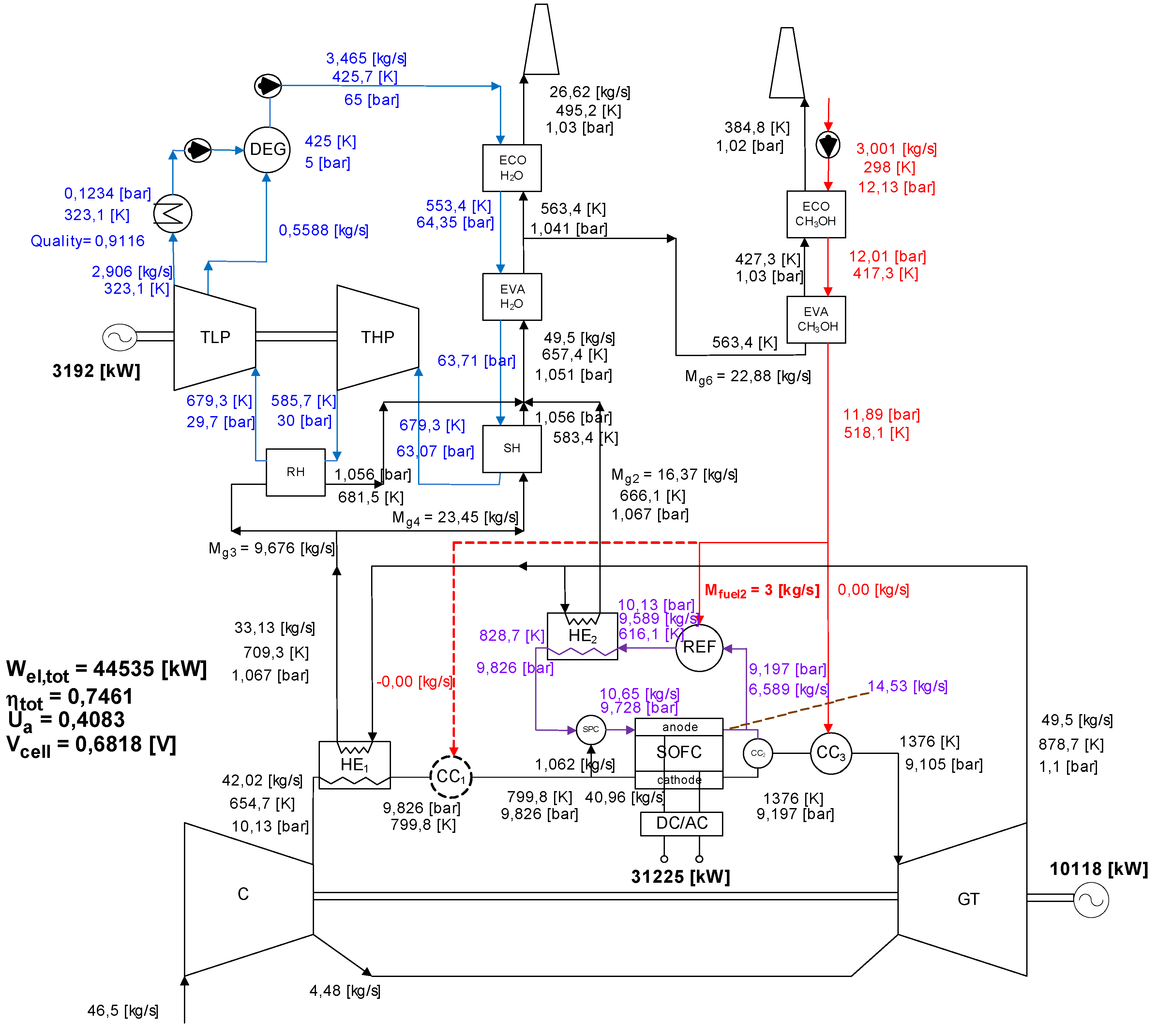
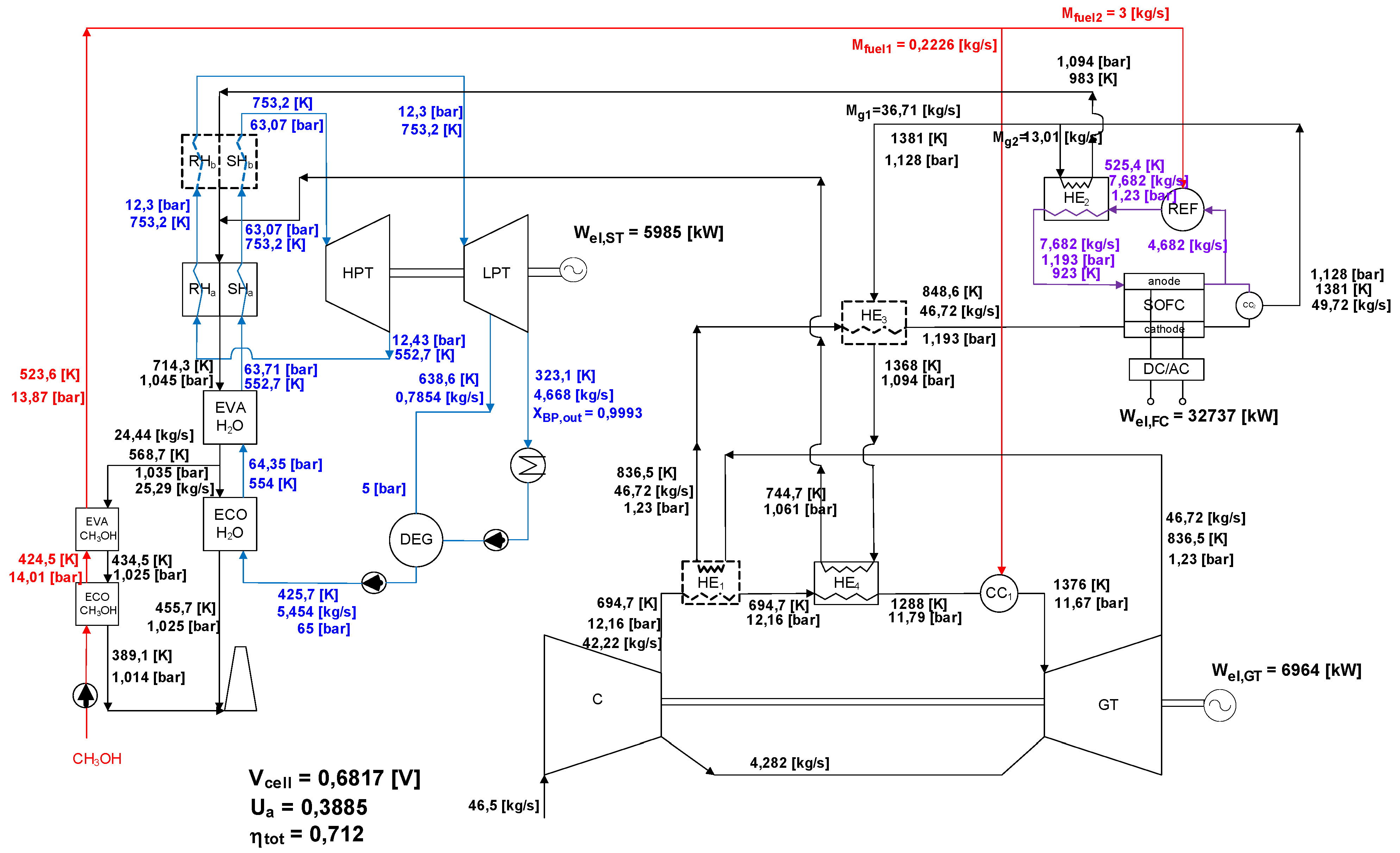
3.1. Case 4—Fuel Cell/Gas Turbine Integration—Reforming of Methanol

The conversion of the chemical exergy of a fuel into electricity implies large irreversibilities, which can be reduced through a careful application of exergy analysis including reactive sub-systems and components. The reference cases here proposed considers Fuel Cell/Gas Turbine power cycle integration. The first case (A) is based on a pressurized Solid Oxide Fuel Cell (SOFC) coupled to a GTCC power cycle (Figure 13), whereas in the second case (B, Figure 14), the SOFC is placed downstream the gas turbine (GT) at atmospheric conditions, and the exhaust of the GT is directed to the SOFC cathode.

The GT is a GE10 model fuelled with methanol, which is attractive because of its low reforming temperature (about 300 °C) and good storability, as it is in liquid state at environmental conditions; moreover, it can be produced as a synthetic fuel from a number of natural resources, including coal and biomass. An extensive description of the proposed power cycles is reported in [22]. Here, the discussion is only focused on exergy analysis and the data shown on Figure 13 and Figure 14 are referred to optimized working conditions. In Figure 13 and Figure 14, W_el,tot is the overall power plant electric power output, η_tot the overall power plant efficiency, U_a is the oxidizer utilization factor (the ratio between the actual mass of reactive oxidizer and the overall input) and V_cell is the fuel cell potential. Exergy analysis applied to these reactive power cycles is able to assess the influence of SOFC and of the heat exchangers network on the overall power plant efficiency at variable working conditions (i.e., pressure ratio β, Figure 15). Three pressure ratios were taken into account: very low value (β = 6), which optimizes the efficiency at low SOFC size (m_fuel,2 = 1 kg/s), β = 10 for SOFC-GTCC-A and β = 12 for SOFC-GTCC-B, the optimizing values at high SOFC size (m_fuel,2 = 3 kg/s) and β = 15, the design value of GT10 [22].

Figure 13. Layout and main parameters for the pressurized SOFC-GTCC-A power cycle.

Figure 13. Layout and main parameters for the pressurized SOFC-GTCC-A power cycle.

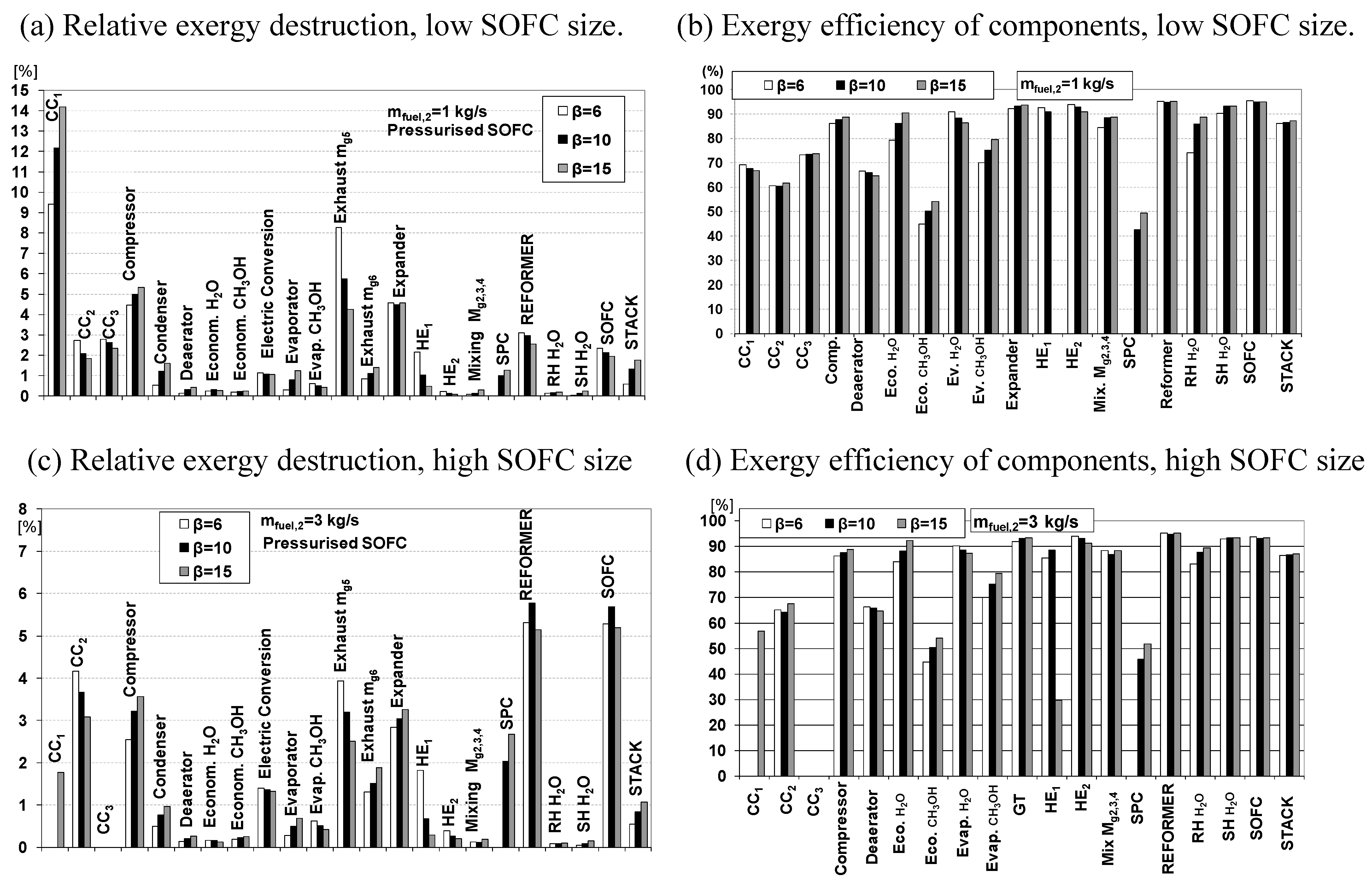
3.2. Exergy Analysis of SOFC-GTCC-A (Pressurized SOFC).

It is interesting to observe the trend of the exergy efficiency of each component under the different working conditions (Figure 15b). The less efficient ones are the combustion chambers, the de-aerator and the methanol economizer. Anyway, the last two have a modest influence on the overall power cycle (less than 0.5%, see Figure 15a). Into the Syngas Pre Combustor (SPC), partial combustion of the produced syngas takes place to reach the required anode temperature if the exhaust temperature is not enough (depending on the GT pressure ratio and firing temperature) to achieve the required value of syngas temperature at anode inlet by heat recovery in HE₂. It is the less efficient component (exergy efficiency lower than 50%). Also the combustion chambers show relatively low exergy efficiencies (70%), as well as the reformer and the GT compressor (80%).

The heat exchangers showing the highest values of exergy destructions are HE₁, HE₂ and the vaporizers. The accurate choice of matched heat capacities on the two sides of HE₂ , which involved adjusting the hot stream flow rate [22], leads to a high exergy efficiency level (90%). Also the heat capacities on the two sides of HE₁ are well matched, as it shows rather good efficiency (85%) except at relatively high pressure ratios. At β = 15, the efficiency of HE₁ drops to 30%, but the heat transferred in this case is relatively modest, which implies a very reduced contribution to the overall power cycle exergy destruction (0.29%). The choice of using the whole exhaust flow rate to feed the vaporizer of the bottoming cycle improved the matching of gas/steam heat capacities [22], which lead to high efficiency level (about 90%) of the vaporizer (EVA_H2O). Low efficiency level is achieved into the methanol economizer (ECO_CH3OH), due to the high difference between exhausts and fuel and not high matching of heat capacities.

Figure 14. Layout and main parameters for the atmospheric SOFC-GTCC-B power cycle.

Figure 14. Layout and main parameters for the atmospheric SOFC-GTCC-B power cycle.

With increasing SOFC size (which is reflected by the fuel input m_fuel,2), the stack exergy loss, and the reformer and combustion chamber CC₂ exergy destructions increase, whereas the compressor and expander ones remain practically unchanged (Figure 15c). The combustor CC₃ is still inactive, whereas CC₁ is only activated at β = 15, but the power output in this case is lower than in the case with low SOFC size; consequently the relative exergy destruction is much reduced. The Pre-combustor relative exergy destruction (SPC) is higher than 2%, as the syngas flow rate—which must be preheated—is increased. The exergy efficiency of the SPC is still very low (50%). The exergy efficiency of power plant components like compressor, expanders, is at the same level of the case with m_fuel,2 = 1 kg/s, which reveals a modest influence of SOFC size on their performance (Figure 15d). On the whole, the overall performance of the power plant is improved increasing the SOFC size (the SOFC is a very exergy-efficient component).

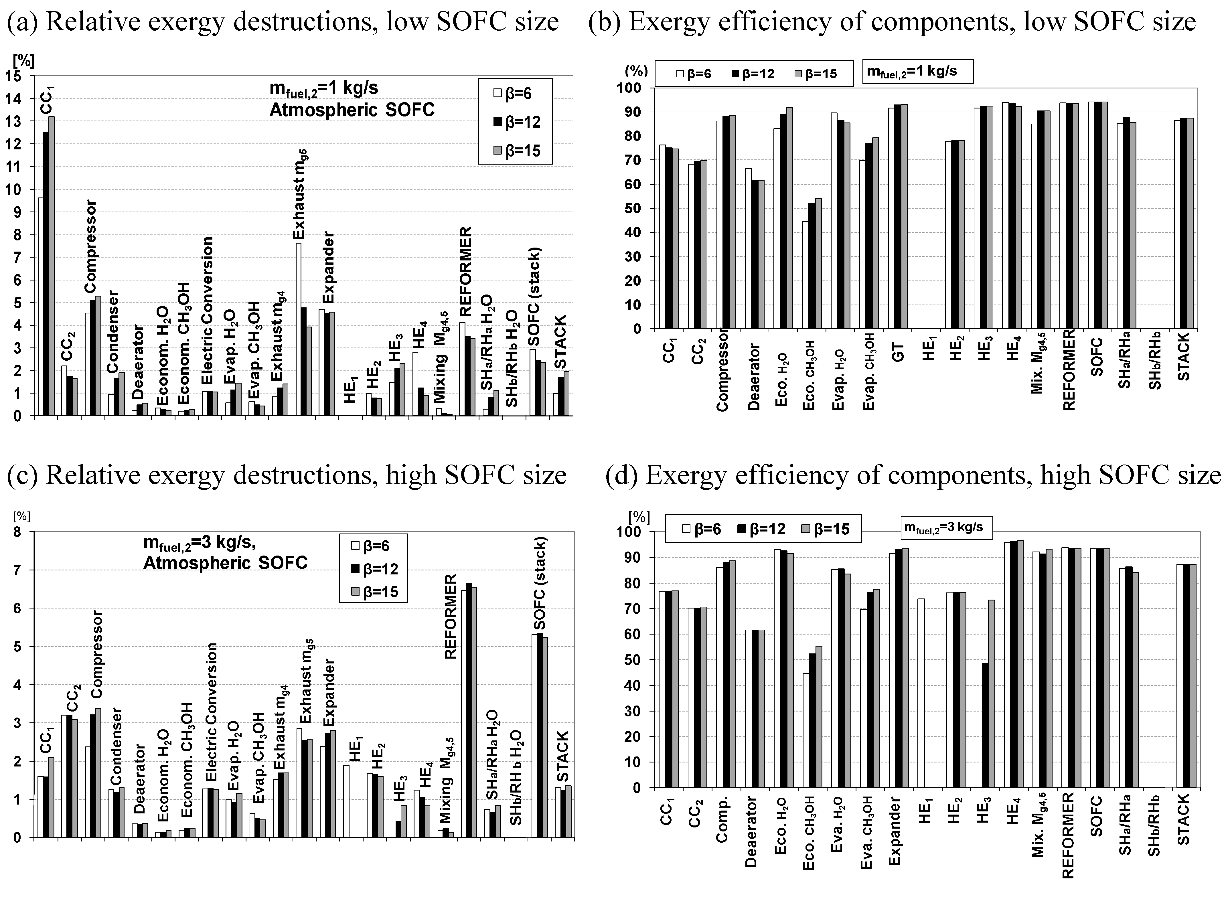
3.3. Exergy Analysis of SOFC-GTCC-B (Atmospheric SOFC)

The relative exergy destructions and the exergy efficiency of SOFC-GTCC-B components (atmospheric SOFC) at small and large SOFC size (m_fuel,2 = 1 and 3 kg/s respectively) are shown in Figure 16. At low SOFC size, the highest exergy destruction is located at the GT combustion chamber CC₁. Like in the previous case A, at low SOFC size the temperature required at the cathode inlet is increased, thus heat exchanger HE₃ is activated and hot exhausts coming from CC₂ get into HE₄ with reduced temperature values, thus the GT heat recuperation is reduced as well. In this way, a higher amount of fuel is required and consequently CC₁ shows a larger exergy destruction. Compressor, reformer, GT expander, and SOFC have a significant weight in the overall power plant exergy balance, even though the last ones have a relatively high efficiency (93–94%, Figure 16b and Figure 16d). In the heat exchangers network, HE₃ and HE₄ have the highest influence on overall exergy destructions, in spite of their high efficiency (>90%).

Figure 15. Relative exergy destruction and exergy efficiency of the SOFC-GTCC-A power cycle components (pressurized SOFC).

Figure 15. Relative exergy destruction and exergy efficiency of the SOFC-GTCC-A power cycle components (pressurized SOFC).

Like in the case of pressurized SOFC, increasing the SOFC size leads to an increase in SOFC and reformer relative exergy destructions (Figure 16a and Figure 16c), with contributions at the same levels as those found in case A with a pressurized SOFC. The exergy destruction in CC₁ is strongly reduced because the GT cycle heat recovery level through HE₄ is consistently increased. The exergy destruction in HE₂ increases due to the higher flowrate of reformed gas. Also HE₁ (when activated, β = 6) provides an appreciable contribution of 2% to the overall exergy destruction. Generally, for higher SOFC flow rates, the power cycle efficiency is improved, mainly due to the higher weight of reformer and SOFC, which are the most efficient components (Figure 16b and Figure 16d).

The exergy efficiency of HE₂ is lower compared to the cycle with pressurized SOFC (76% vs. 92%), due to the much larger average temperature difference between the hot and cold streams (400 °C vs. 50 °C).

Figure 16. Relative exergy destructions and exergy efficiency of the SOFC-GTCC-B power cycle components (Atmospheric SOFC).

Figure 16. Relative exergy destructions and exergy efficiency of the SOFC-GTCC-B power cycle components (Atmospheric SOFC).

4. Conclusions

Several cases of possible improvement of energy conversion/utilization systems through exergy analysis have been presented and discussed. The selected cases range from conventional power plants (with application of optimization tools), to renewable energy systems (solar energy, with attention to control law for solar thermal conversion; and solar collectors design and operation); finally, more complicated applications involving reactive systems–using methanol and an hybrid GT/SOFC chemically recuperated cycle-have been presented.

The purpose of this paper—which presents mostly un-published material from a long time span of the Authors’ research—is to demonstrate the potential of exergy analysis applied to energy conversion/utilization systems. The use of the exergy method is much more widespread in the scientific community than 20 or 30 years ago, and a solid scientific background has been developed, as confirmed by the existence of several reference textbooks [1,2,3,4,18]; however, the potential of exergy analysis has not yet been completely demonstrated and the Authors hope that this paper can represent a small contribution to this end.

References

1. Bejan, A.; Tsatsaronis, G.; Moran, M. Thermal Design and Optimization; Wiley Interscience: New York, NY, USA, 1996. [Google Scholar]
2. Kotas, T.J. The Exergy Method of Thermal Plant Analysis; Krieger: New York, NY, USA, 1995. [Google Scholar]
3. Szargut, J.; Morris, D.R.; Stewart, F.R. Exergy Analysis of Thermal, Chemical and Metallurgical Processes; Hemisphere: New York, NY, USA, 1988. [Google Scholar]
4. Moran, M. Availability Analysis: A Guide to Efficient Energy Usage; Prentice-Hall: Upper Saddle River, NJ, USA, 1982. [Google Scholar]
5. Ahern, J.E. The Exergy Method of Energy System Analysis; Wiley: New York, NY, USA, 1980. [Google Scholar]
6. Kotas, T.J. The Exergy Method of Thermal Plant Analysis, Reprint ed.; Krieger: Malabar, FL, USA, 1995. [Google Scholar]
7. F-Chart Software. Available online: http://www.fchart.com/ees/ees.shtml (accessed on December 31, 2009).
8. Odeh, S.D. Unified model of solar thermal electric generation systems. Renewable Energy 2003, 28, 755–767. [Google Scholar] [CrossRef]
9. Mills, D. Advances in solar thermal electricity technology. Sol. Energy 2004, 76, 19–31. [Google Scholar] [CrossRef]
10. Camacho, E.; Berenguel, M.; Rubio, F.R. Advanced Control of Solar Plants; Springer-Verlag: London, UK, 1997. [Google Scholar]
11. Duffie, J.A.; Beckman, W.A. Solar Energy Thermal Processes; Wiley: New York, NY, USA, 1984. [Google Scholar]
12. Therminol. Heat Transfer Fluids by Solutia. Available online: http://www.therminol.com (accessed on 31 December, 2009).
13. Manfrida, G.; Kawambwa, S. A two-phase solar collector powering a rankine organic cycle. In Presented at World Renewable Energy Congress, Reading, UK, September 1990.
14. ARCHIMEDE—ENEA Grande Progetto Solare Termodinamico. Available online: http://www.enea.it/com/solar/index.html (accessed on 31 December, 2009).
15. Valenzuela, M.; Zarza, E.; Berenguel, M.; Camacho, E.F. Control concepts for direct steam generation in parabolic troughs. Sol. Energy 2005, 78, 301–311. [Google Scholar] [CrossRef]
16. Manfrida, G. The choice of the optimal working point for solar collectors. Sol. Energy 1985, 34, 6. [Google Scholar] [CrossRef]
17. Manfrida, G.; Kawambwa, S. Exergy control for a flat-plate collector/Rankine cycle solar power system. J. Sol. Energy Eng. 1991, 113, 89–93. [Google Scholar] [CrossRef]
18. Schuster, A.; Karellas, S; Kakaras, E.; Spliethoff, H. Energetic and economic investigation of Organic Rankine Cycle applications. Appl. Therm. Eng. 2009, 29, 8–9, 1809–1817. [Google Scholar] [CrossRef]
19. Bejan, A. Entropy Generation Through Heat and Fluid Flow; Wiley: New York, NY, USA, 1982. [Google Scholar]
20. Farahat, S.; Sarhaddi, F.; Ajam, F. Exergetic optimization of flat plate solar collector. Renewable Energy 2008, 34, 1169–1174. [Google Scholar] [CrossRef]
21. Baldini, A.; Manfrida, G.; Tempesti, D. Model of a solar collector/storage system for industrial thermal applications. In ECOS Conference, Krakow, Poland, June 2008.
22. Fiaschi, D.; Manfrida, G.; Anselmi, S. Performance analysis and comparison of hybrid SOFC-GT cycles fuelled with methanol. In ASME paper IGTI Turbo GT2008-51367, Berlin, Germany, June 2008.