Wiretap Channel with Action-Dependent Channel State Information

Abstract
:1. Introduction


2. Notations, Definitions and the Main Results
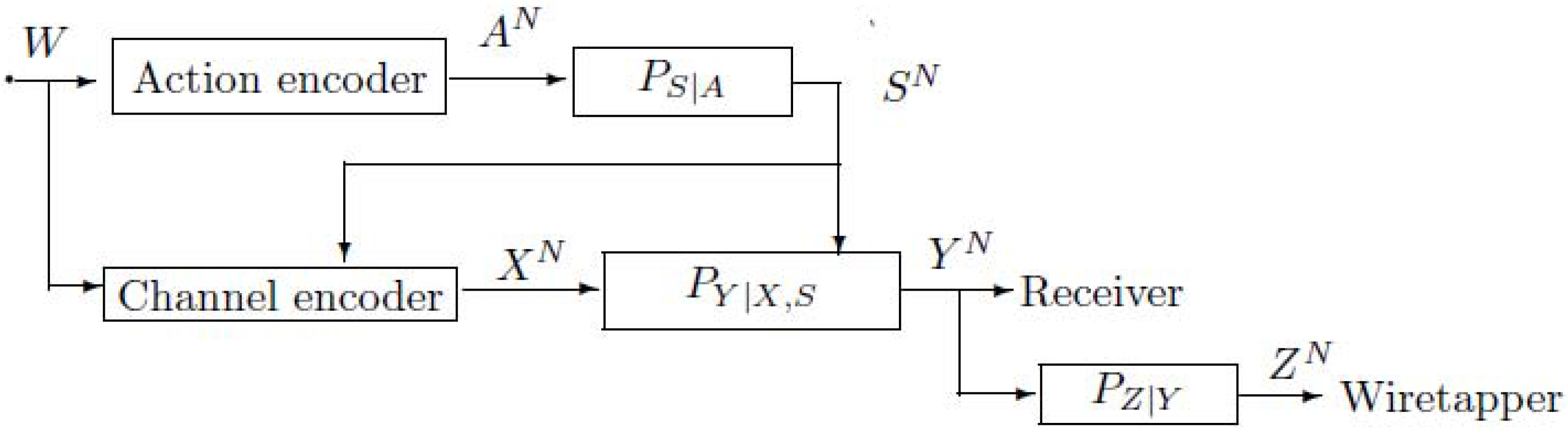
2.1. The Model of Figure 4 with Noncausal Channel State Information
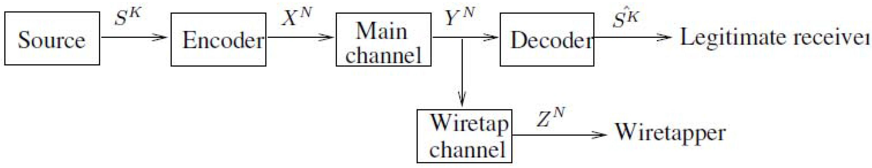
- The formula in Theorem 1 implies that the wiretapper obtains the information about the message not only from the codeword transmitted in the channels, but also from the action sequence . If the wiretapper knows , he knows the corresponding message.
- The region is convex, and the proof is directly obtained by introducing a time sharing random variable into Theorem 1, and therefore, we omit the proof here.
- Secrecy capacityThe points in for which are of considerable interest, which imply the perfect secrecy . Clearly, we can easily bound the secrecy capacity of the model of Figure 4 with noncausal channel state information byProof 1 (Proof of (7)) Substituting into the region in Theorem 1, we haveNote that the pair is achievable, and therefore, the secrecy capacity . Thus the proof is completed.
- The region is convex, and the proof is similar to that of Theorem 1. Therefore, we omit the proof here.
- Observing the formula in Theorem 2, we havewhere (a) is from the fact that , and (b) is from the Markov chain . Then it is easy to see that .
- The secrecy capacity of the model of Figure 4 with noncausal channel state information is upper bounded byThe upper bound is easily obtained by substituting into the region in Theorem 2, and therefore, we omit the proof here.
2.2. The Model of Figure 4 with Causal Channel State Information
- The region is convex.
- The range of the random variable U satisfiesThe proof is similar to that in Theorem 1, and it is omitted here.
- Secrecy capacityThe points in for which are of considerable interest, which imply the perfect secrecy . Clearly, we can easily bound the secrecy capacity of the model of Figure 4 with causal channel state information byProof 2 (Proof of (15)) Substituting into the region in Theorem 3, we haveNote that the pair is achievable, and therefore, the secrecy capacity . Thus the proof is completed.
- The region is convex.
- The ranges of the random variables U, V and K satisfyThe proof is similar to that in Section D, and it is omitted here.
- The secrecy capacity of the model of Figure 4 with causal channel state information is upper bounded byThe upper bound is easily obtained by substituting into the region in Theorem 4, and therefore, we omit the proof here.
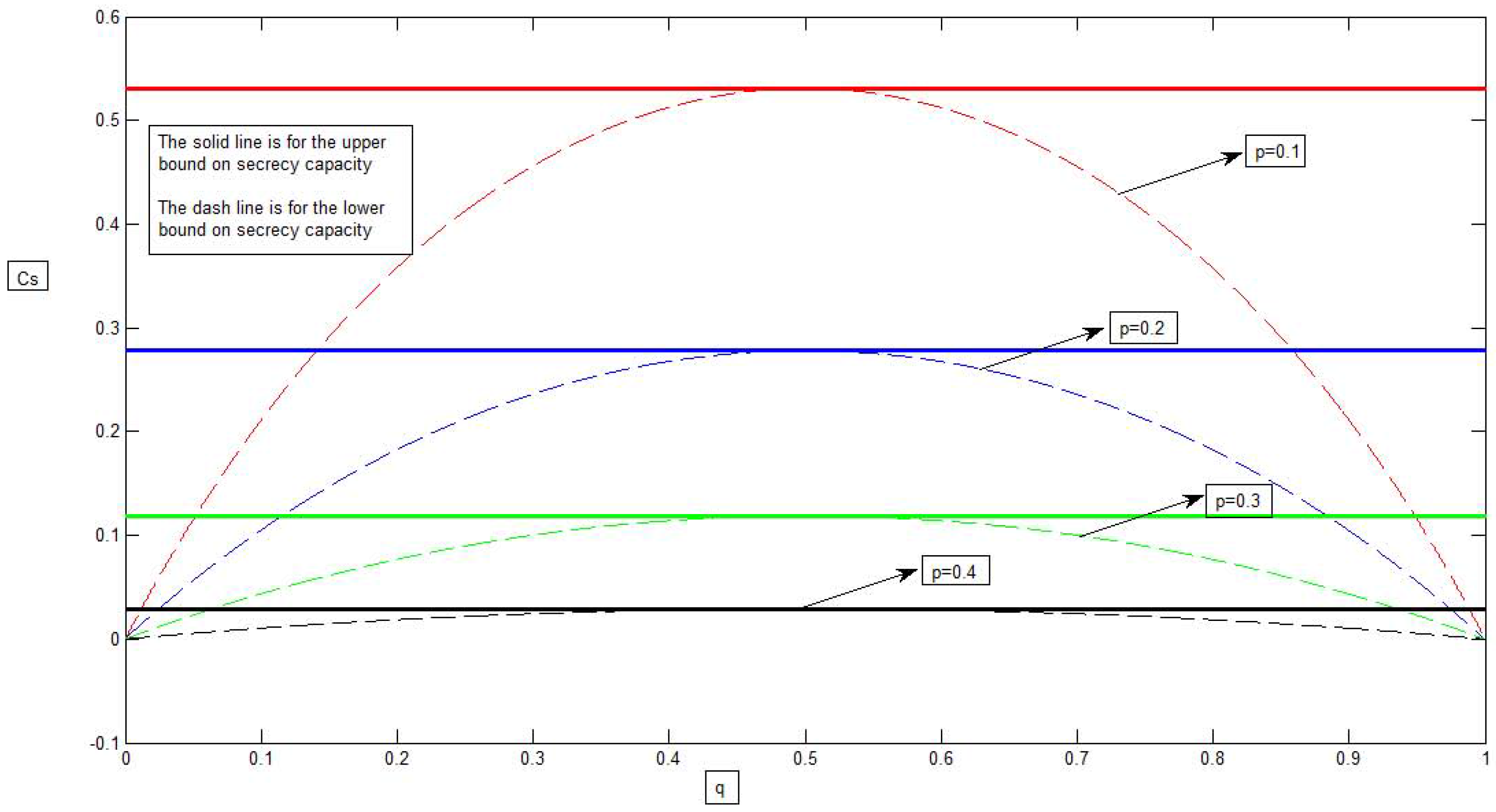
3. A Binary Example for the Model of Figure 4 with Causal Channel State Information
4. Conclusions
Acknowledgement
References
- Shannon, C.E. Channels with side information at the transmitter. IBM J. Res. Dev. 1958, 2, 289–293. [Google Scholar] [CrossRef]
- Kuznetsov, N.V.; Tsybakov, B.S. Coding in memories with defective cells. Probl. Peredachi Informatsii 1974, 10, 52–60. [Google Scholar]
- Gel’fand, S.I.; Pinsker, M.S. Coding for channel with random parameters. Problems. Control Inf. Theory 1980, 9, 19–31. [Google Scholar]
- Costa, M.H.M. Writing on dirty paper. IEEE Trans. Inf. Theory 1983, 29, 439–441. [Google Scholar] [CrossRef]
- Weissman, T. Capacity of channels with action-dependent states. IEEE Trans. Inf. Theory 2010, 56, 5396–5411. [Google Scholar] [CrossRef]
- Wyner, A.D. The wire-tap channel. Bell Syst. Tech. J. 1975, 54, 1355–1387. [Google Scholar] [CrossRef]
- Csisz´r, I.; Körner, J. Broadcast channels with confidential messages. IEEE Trans. Inf. Theory 1978, 24, 339–348. [Google Scholar]
- Körner, J.; Marton, K. General broadcast channels with degraded message sets. IEEE Trans. Inf. Theory 1977, 23, 60–64. [Google Scholar] [CrossRef]
- Leung-Yan-Cheong, S.K.; Hellman, M.E. The Gaussian wire-tap channel. IEEE Trans. Inf. Theory 1978, 24, 451–456. [Google Scholar] [CrossRef]
- Mitrpant, C.; Han Vinck, A.J.; Luo, Y. An achievable region for the gaussian wiretap channel with side information. IEEE Trans. Inf. Theory 2006, 52, 2181–2190. [Google Scholar] [CrossRef]
- Chen, Y.; Han Vinck, A.J. Wiretap channel with side information. IEEE Trans. Inf. Theory 2008, 54, 395–402. [Google Scholar] [CrossRef]
- Dai, B.; Luo, Y. Some new results on wiretap channel with side information. Entropy 2012, 14, 1671–1702. [Google Scholar] [CrossRef]
- Csisz´r, I.; Körner, J. Information Theory: Coding Theorems for Discrete Memoryless Systems; Academic: London, UK, 1981; pp. 123–124. [Google Scholar]
A. Proof of Theorem 1
A.1. Code Construction
- (Case 1) If , double binning technique [11] is used in the construction of the code-book.
- (Case 2) If , Gel’fand-Pinsker’s binning technique [3] is used in the construction of the code-book.
- (Code construction for Case 1)Given a pair , choose a joint probability mass function such thatThe message set satisfies the following condition:where γ is a fixed positive real numbers andNote that (a) is from and (A1). Let .Code-book generation:
- –
- (Construction of )Generate i.i.d. sequences , according to the probability mass function . Index each sequence by . For a given message w (), choose a corresponding as the output of the action encoder.
- –
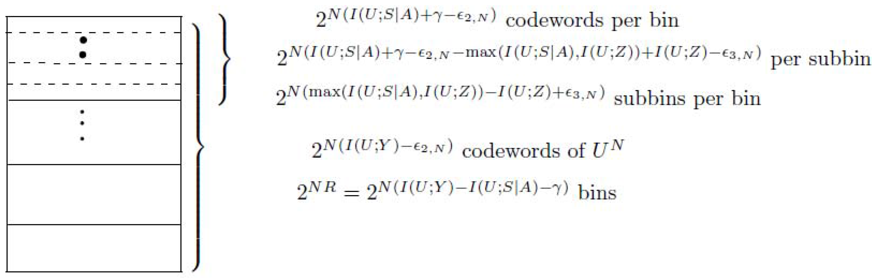
- (Construction of )For the transmitted action sequence , generate ( as ) i.i.d. sequences , according to the probability mass function . Distribute these sequences at random into bins such that each bin contains sequences. Index each bin by . Then place the sequences in every bin randomly into ( as ) subbins such that every subbin containssequences. Let J be the random variable to represent the index of the subbin. Index each subbin by, i.e.,Here note that the number of the sequences in every subbin is upper bounded as follows.where (a) is from (A2). This implies thatNote that (A5) can be proved by using Fano’s inequality and (A4).Let be the state sequence generated in response to the action sequence . For a given message w () and channel state , try to find a sequence in bin w such that . If multiple such sequences in bin w exist, choose the one with the smallest index in the bin. If no such sequence exists, declare an encoding error.Figure A1 shows the construction of for case 1, see the following.
- –
- (Construction of ) The is generated according to a new discrete memoryless channel (DMC) with inputs , , and output . The transition probability of this new DMC is , which is obtained from the joint probability mass function . The probabilityis calculated as follows.
Decoding:Given a vector , try to find a sequence such that . If there exist sequences with the same , put out the corresponding . Otherwise, i.e., if no such sequence exists or multiple sequences have different message indices, declare a decoding error. - (Code construction for Case 2)Given a pair , choose a joint probability mass function such thatThe message set satisfies the following condition:where is a fixed positive real numbers andNote that (b) is from and (A7). Let .Code-book generation:
- –
- (Construction of )Generate i.i.d. sequences , according to the probability mass function . Index each sequence by . For a given message w (), choose a corresponding as the output of the action encoder.
- –
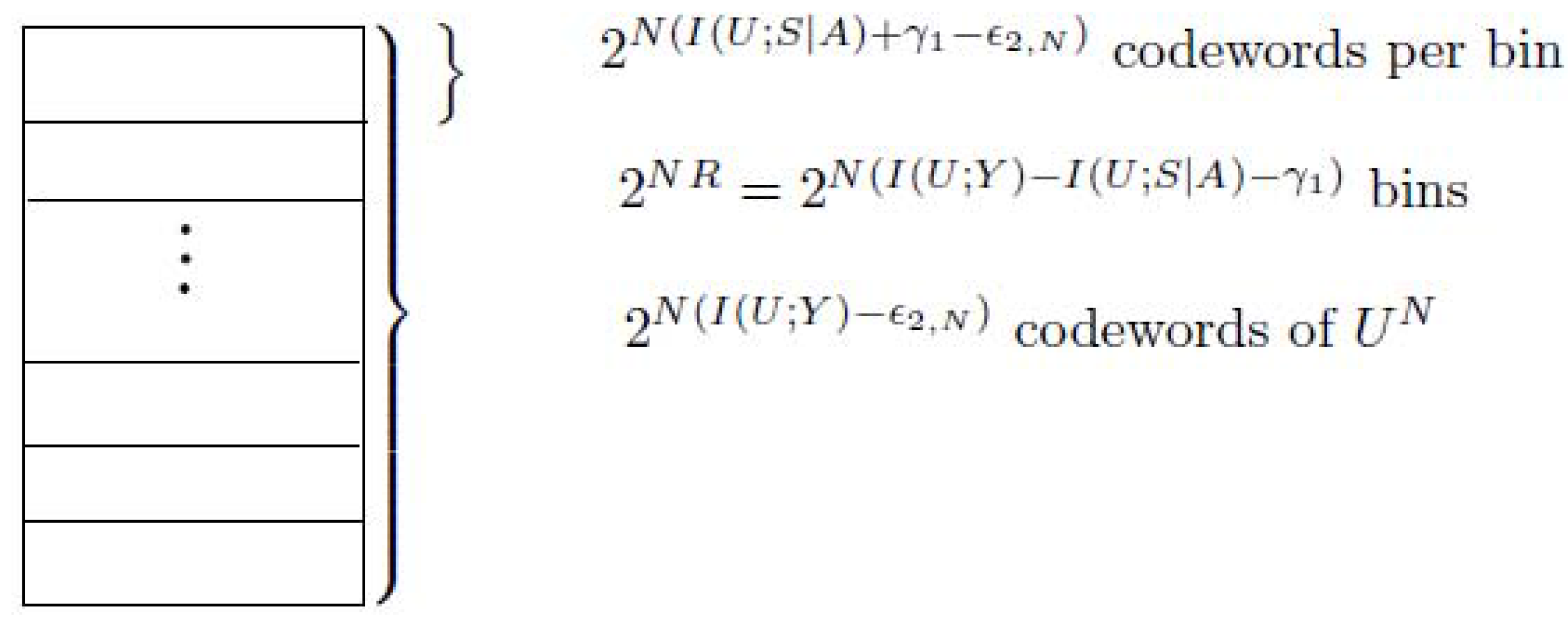
- (Construction of )For the transmitted action sequence , generate ( as ) i.i.d. sequences , according to the probability mass function . Distribute these sequences at random into bins such that each bin contains sequences. Index each bin by .Let be the state sequence generated in response to the action sequence . For a given message w () and channel state , try to find a sequence in bin w such that . If multiple such sequences in bin w exist, choose the one with the smallest index in the bin. If no such sequence exists, declare an encoding error.Figure A2 shows the construction of for case 2, see the following.
- –
- (Construction of ) The is generated the same as that for the case 1, and it is omitted here.
Decoding:Given a vector , try to find a sequence such that . If there exist sequences with the same , put out the corresponding . Otherwise, i.e., if no such sequence exists or multiple sequences have different message indices, declare a decoding error.
A.2. Proof of Achievability
B. Proof of Theorem 2
C. Size Constraint of The Random Variables in Theorem 1
D. Size Constraint of The Random Variables in Theorem 2
- (Proof of )LetDefine the following continuous scalar functions of :Since there are functions of , the total number of the continuous scalar functions of is +1.Let . With these distributions , we haveAccording to the support lemma ([13], p.310), the random variable U can be replaced by new ones such that the new U takes at most different values and the expressions (A36), (A37) and (A38) are preserved.
- (Proof of )LetDefine the following continuous scalar functions of :Since there are functions of , the total number of the continuous scalar functions of is .Let . With these distributions , we haveAccording to the support lemma ([13], p.310), the random variable V can be replaced by new ones such that the new V takes at most different values and the expressions (A40) and (A41) are preserved.
- (Proof of )Once the alphabet of V is fixed, we apply similar arguments to bound the alphabet of K, see the following. Define continuous scalar functions of :where of the functions , only are to be considered.For every fixed v, let . With these distributions , we haveBy the support lemma ([13], p.310), for every fixed v, the size of the alphabet of the random variable K can not be larger than , and therefore, is proved.
E. Proof of Theorem 3
E.1. Code Construction
- (Case 1) If , Wyner’s random binning technique [6] is used in the construction of the code-book.
- (Case 2) If , Shannon’s strategy [1] is used in the construction of the code-book.
- (Code construction for case 1)Given a pair , choose a joint probability mass function such thatThe message set satisfies the following condition:where γ is a fixed positive real numbers andNote that (a) is from and (A44). Let .Code-book generation:
- –
- (Construction of )Generate i.i.d. sequences , according to the probability mass function . Index each sequence by . For a given message w (), choose a corresponding as the output of the action encoder.
- –
- (Construction of )For the transmitted action sequence , generate ( as ) i.i.d. sequences , according to the probability mass function . Distribute these sequences at random into bins such that each bin contains sequences. Index each bin by .Here note that the number of the sequences in every bin is upper bounded as follows.where (a) is from (A45). This implies thatNote that (A47) can be proved by using Fano’s inequality and (A46).For a given message w (), randomly choose a sequence in bin w as the realization of .Let be the state sequence generated in response to the action sequence .
- –
- (Construction of ) The is generated according to a new discrete memoryless channel (DMC) with inputs , , and output . The transition probability of this new DMC is , which is obtained from the joint probability mass function . The probabilityis calculated as follows.
Decoding:Given a vector , try to find a sequence such that . If there exist sequences with the same , put out the corresponding . Otherwise, i.e., if no such sequence exists or multiple sequences have different message indices, declare a decoding error. - (Code construction for case 2)Given a pair , choose a joint probability mass function such thatThe message set satisfies the following condition:where is a fixed positive real numbers andNote that (b) is from and (A49). Let .Code-book generation:
- –
- (Construction of )Generate i.i.d. sequences , according to the probability mass function . Index each sequence by . For a given message w (), choose a corresponding as the output of the action encoder.
- –
- (Construction of )For the transmitted action sequence , generate i.i.d. sequences , according to the probability mass function . Index each by .For a given message w (), choose a sequence as the realization of .Let be the state sequence generated in response to the action sequence .
- –
- (Construction of ) The is generated the same as that for the case 1, and it is omitted here.
Decoding:Given a vector , try to find a sequence such that . If there exist sequences with the same , put out the corresponding . Otherwise, i.e., if no such sequence exists or multiple sequences have different message indices, declare a decoding error.
E.2. Proof of Achievability
F. Proof of Theorem 4
© 2013 by the authors; licensee MDPI, Basel, Switzerland. This article is an open access article distributed under the terms and conditions of the Creative Commons Attribution license (http://creativecommons.org/licenses/by/3.0/).
Share and Cite
Dai, B.; Vinck, A.J.H.; Luo, Y.; Tang, X. Wiretap Channel with Action-Dependent Channel State Information. Entropy 2013, 15, 445-473. https://doi.org/10.3390/e15020445
Dai B, Vinck AJH, Luo Y, Tang X. Wiretap Channel with Action-Dependent Channel State Information. Entropy. 2013; 15(2):445-473. https://doi.org/10.3390/e15020445
Chicago/Turabian StyleDai, Bin, A. J. Han Vinck, Yuan Luo, and Xiaohu Tang. 2013. "Wiretap Channel with Action-Dependent Channel State Information" Entropy 15, no. 2: 445-473. https://doi.org/10.3390/e15020445