Information Theory Analysis of Cascading Process in a Synthetic Model of Fluid Turbulence


Abstract
: The use of transfer entropy has proven to be helpful in detecting which is the verse of dynamical driving in the interaction of two processes, X and Y. In this paper, we present a different normalization for the transfer entropy, which is capable of better detecting the information transfer direction. This new normalized transfer entropy is applied to the detection of the verse of energy flux transfer in a synthetic model of fluid turbulence, namely the Gledzer–Ohkitana–Yamada shell model. Indeed, this is a fully well-known model able to model the fully developed turbulence in the Fourier space, which is characterized by an energy cascade towards the small scales (large wavenumbers k), so that the application of the information-theory analysis to its outcome tests the reliability of the analysis tool rather than exploring the model physics. As a result, the presence of a direct cascade along the scales in the shell model and the locality of the interactions in the space of wavenumbers come out as expected, indicating the validity of this data analysis tool. In this context, the use of a normalized version of transfer entropy, able to account for the difference of the intrinsic randomness of the interacting processes, appears to perform better, being able to discriminate the wrong conclusions to which the “traditional” transfer entropy would drive.1. Introduction
This paper is about the use of quantities, referred to as information dynamical quantities (IDQ), derived from the Shannon information [1] to determine cross-predictability relationships in the study of a dynamical system. We will refer to as “cross-predictability” the possibility of predicting the (near) future behavior of a process, X, by observing the present behavior of a process, Y, likely to be interacting with X. Observing X given Y is of course better than observing only X, as far as predicting X is concerned: it will be rather interesting to compare how the predictability of X is increased given Y with the increase of predictability of Y given X. To our understanding, this cross-predictability analysis (CPA) gives an idea of the verse of dynamical driving between Y and X. In particular, the data analysis technique presented here is tested on a synthetic system completely known by construction. The system at hand is the Gledzer–Ohkitana–Yamada (GOY) shell model, describing the evolution of turbulence in a viscous incompressible fluid. In this model, the Fourier component interaction takes place locally in the space of wavenumbers, and due to dissipation growing with k, a net flux of energy flows from the larger to the smaller scales (direct cascade). A dynamical “driving” of the large on the small scales is then expected, which is verified here through simulations: mutual information and transfer entropy analysis are applied to the synthetic time series of the Fourier amplitudes that are interacting.
The purpose of applying a certain data analysis technique to a completely known model is to investigate the potentiality of the analysis tool in retrieving the expected information, preparing it for future applications to real systems. The choice of the GOY model as a test-bed for the IDQ-based CPA is due both to its high complexity, rendering the test rather solid with respect to the possible intricacies expected in natural systems, and to its popularity in the scientific community, due to how faithfully it simulates real features of turbulence.
In order to focus on how IDQ-based CPA tools are applied in the study of coupled dynamical processes, let us consider two processes, X and Y, whose proxies are two physical variables, x and y, evolving with time, and let us assume that the only thing one measures are the values, x (t) and y (t), as time series. In general, one may suppose the existence of a stochastic dynamical system (SDS) governing the interaction between X and Y, expressed mathematically as:
where the terms, f and g, contain stochastic forces rendering the dynamics of x and y probabilistic [2]. Actually, the GOY model studied here is defined as deterministic, but the procedures discussed are perfectly applicable, in principle, to any closed system in the form of (1). The sense of applying probabilistic techniques to deterministic processes is that such processes may be so complicated and rich, that a probabilistic picture is often preferable, not to mention the school of thought according to which physical chaos is stochastic, even if formally deterministic [3,4]. Indeed, since real-world measurements always have finite precision and most of the real-world systems are highly unstable (according to the definition of Prigogine and his co-workers), deterministic trajectories turn out to be unrealistic, hence an unuseful tool to describe reality.
Through the study of the IDQs obtained from x (t) and y (t), one may, for example, hope to deduce whether the dependence of xÿ on y is “stronger” than the dependence of yÿ on x, hence how Y is driving X.
The IDQs discussed here have been introduced and developed over some decades. After Shannon’s work [1], where the information content of a random process was defined, Kullback used it to make comparisons between different probability distributions [5], which soon led to the definition of mutual information (MI) as a way to quantify how much the two processes deviate from statistical independence. The application of MI to time series analysis appears natural: Kantz and Schreiber defined and implemented a set of tools to deduce dynamic properties from observed time series (see [6] and the references therein), including time-delayed mutual information.
The tools of Kantz and Schreiber were augmented in [7] with the introduction of the so-called transfer entropy (TE): information was no longer describing the underdetermination of the system observed, but rather, the interaction between two processes studied in terms of how much information is gained on the one process observing the other, i.e., in terms of information transfer. An early review about the aforementioned IDQs can be found in [8].
TE was soon adopted as a time series analysis tool in many complex system fields, such as space physics [9,10] and industrial chemistry [11], even if Kaiser and Schreiber developed a criticism and presented many caveats to the extension of the TE to continuous variables [12]. Since then, however, many authors have been using TE to detect causality, for example, in stock markets [13], symbolic dynamics [14], biology and genetics [15] and meteorology [16,17]. In the field of neuroscience, TE has been applied broadly, due to the intrinsic intricacy of the matter [18], and recently extended to multi-variate processes [19].
A very important issue is, namely, the physical meaning of the IDQs described before. Indeed, while the concept of Shannon entropy is rather clear and has been related to the thermodynamical entropy in classical works, such as [20], mutual information and transfer entropy have not been clearly given yet a significance relevant for statistical mechanics. The relationship between TE and the mathematical structure of the system (1) has been investigated in [16], while a more exhaustive study on the application of these information theoretical tools to systems with local dynamics is presented in [21] and the references therein. This “physical sense” of the IDQs will be the subject of our future studies.
The paper is organized as follows.
A short review of the IDQs is done in Section 2. Then, the use of MI and TE to discriminate the “driver” and the “driven” process is criticized, and new normalized quantities are introduced, more suitable for analyzing the cross-predictability in dynamical interactions of different “intrinsic” randomness (normalizing the information theoretical quantities, modifying them with respect to their initial definitions, is not a new thing: in [22], the transfer entropy is modified, so as to include some basic null hypothesis in its own definition; in [23], the role of information compression in the definitions of IDQs is stressed, which will turn out to emerge in the present paper, as well).
The innovative feature of the IDQs described here is the introduction of a variable delay, τ : the IDQs peak in the correspondence of some τ̃ estimating the characteristic time scale(s) of the interaction, which may be a very important point in predictability matters [24]. The problem of inferring interaction delays via transfer entropy has also been given a rigorous treatment in [25], where ideas explored in [24] are discussed with mathematical rigor.
In Section 3, the transfer entropy analysis (TEA) is applied to synthetic time series obtained from the GOY model of turbulence, both in the form already described, e.g., in [10,24], and in the new normalized version, defined in Section 2. The advantages of using the new normalized IDQs are discussed, and conclusions are drawn in Section 4.
2. Normalized Mutual Information and Transfer Entropy
In all our reasoning, we will use four time series: those representing two processes, x (t) and y (t), and those series themselves time-shifted forward by a certain amount of time, τ. The convenient notation adopted reads:
(in Equation (2) and everywhere, “:=” means “equal by definition”). The quantity, pt (x, y), is the joint probability of having a certain value of x and y at time t; regarding notation, the convention:
is understood.
Shannon entropy is defined for a stochastic process, A, represented by the variable, a,
quantifying the uncertainty on A before measuring a at time t. Since, in practice, discretized continuous variables are often dealt with, all the distributions, pt (a), as in Equation (4), are then probability mass functions (pmfs) rather than probability density functions (pdfs).
For two interacting processes, X and Y, it is worth defining the conditional Shannon information entropy of X given Y :
The instantaneous MI shared by X and Y is defined as:
positive Mt (X, Y ) indicates that X and Y interact. The factorization of probabilities and non-interaction has an important dynamical explanation in stochastic system theory: when the dynamics in Equation (1) is reinterpreted in terms of probabilistic path integrals [26], then the factorization of probabilities expresses the absence of interaction terms in stochastic Lagrangians. Indeed, (stochastic) Lagrangians appear in the exponent of transition probabilities, and their non-separable addenda, representing interactions among sub-systems, are those terms preventing probabilities from being factorizable.
About Mt (X, Y ), one should finally mention that it is symmetric: Mt (X, Y ) = Mt (Y,X).
There may be reasons to choose to use the MI instead of, say, cross-correlation between X and Y : the commonly used cross-correlation encodes only information about the second order momentum, while MI uses all information defined in the probability distributions. Hence, it is more suitable for studying non-linear dependencies [27,28], expected to show up at higher order momenta.
In the context of information theory (IT), we state that a process, Y, drives a process, X, between t and t + τ (with τ > 0) if observing y at the time, t; we are less ignorant of what x at the time, t + τ, is going to be like, than how much we are on y at the time t + τ observing x at the time t. The delayed mutual information (DMI):
turns out to be very useful for this purpose. DMI is clearly a quantity with which cross-predictability is investigated.
In [9], a generalization of DMI is presented and referred to as transfer entropy (TE), by adapting the quantity originally introduced by Schreiber in [7] to dynamical systems, such as Equation (1), and to time delays τ that may be varied, in order to test the interaction at different time scales:
In practice, the TE provides the amount of knowledge added to X at time t + τ, knowing x (t), by the observation of y (t).
The easiest way to compare the two verses of cross-predictability is of course that of taking the difference between the two:
as done in [9,10,24]. The verse of prevailing cross-predictability is stated to be that of information transfer. Some comments on quantities in Equation (9) are necessary.
Consider taking the difference between TY→X (τ ; t) and TX→Y (τ ; t) in order to understand which is the prevalent verse of information transfer: if one of the two processes were inherently more noisy than the other, then the comparison between X and Y via such differences would be uneven, somehow. Since cross-predictability via information transfer is about the efficiency of driving, then the quantities, MY→X (τ ; t) and TY→X (τ ; t), must be compared to the uncertainty induced on the “investigated system” by all the other things working on it and rendering its motion unpredictable, in particular the noises of its own dynamics (here, we are not referring only to the noisy forces on it, but also/mainly to the internal instabilities resulting in randomness). When working with MY→X (τ ; t), this “uncertainty” is quantified by I (Xτ ), while when working with TY→X (τ ; t), the “uncertainty-of-reference” must be It (Xτ |X). One can then define a normalized delayed mutual information (NDMI):
and a normalized transfer entropy (NTE):
or equally:
These new quantities, RY→X (τ ; t) and KY→X (τ ; t), will give a measure of how much the presence of an interaction augments the predictability of the evolution, i.e., will quantify cross-predictability.
The positivity of ΔRY→X (τ ; t) or ΔKY→X (τ ; t) is a better criterion than the positivity of ΔMY→X (τ ; t) or ΔTY→X (τ ; t) for discerning the driving direction, since the quantities involved in RY→X (τ ; t) and KY→X (τ ; t) factorize the intrinsic randomness of a process and try to remove it with the normalization, It (Xτ ) and It (Xτ |X), respectively. Despite this, ΔMY→X (τ ; t) and ΔTY→X (τ ; t) can still be used for that analysis in the case that the degree of stochasticity of X and Y are comparable. Consider for instance that at t + τ, the Shannon entropy of X and Y are equal both to a quantity, I0, and the conditioned ones equal both to J0; clearly, one has:
and the quantity, ΔRY→X (τ ; t), is proportional to ΔMY→X (τ ; t) through a number , so they encode the same knowledge. The same should be stated for ΔKY→X (τ ; t) and ΔTY→X (τ ; t). This is why we claim that the diagnoses in [9,10,24] were essentially correct, even if we will try to show here that the new normalized quantities work better in general.
Before applying the calculation of the quantities, ΔTY→X (τ ; t) and ΔKY→X (τ ; t), to the turbulence model considered in Section 3, it is worth underlining again the dependence of all these IDQs on the delay, τ : the peaks of the IDQs on the τ axis indicate those delays after which the process, X, shares more information with the process, Y, i.e., the characteristic time scales of their cross-predictability, due to their interaction.
3. Turbulent Cascades and Information Theory
This section considers an example in which we know what must be expected, and apply our analysis tools to it to check and refine them. In this case, the application of the normalized quantities instead of the traditional ones revised in Section 2 is investigated in some detail. In the chosen example, the IDQs are used to recognize the existence of cascades in a synthetic model of fluid turbulence [29,30].
Some theoretical considerations are worth being done in advance. The quantities described above are defined using instantaneous pmfs, i.e., pmfs that exist at time t. As a result, the quantities may vary with time. Unfortunately, it is difficult to recover the statistics associated with such PMFs, except in artificial cases, when running ensemble simulations on a computer. When examining real-world systems, for example in geophysics, then this luxury is not available. Hence, in many cases, one can only calculate time statistics rather than ensemble statistics; since any analysis in terms of time statistics is only valid when the underlying system is sufficiently ergodic, what one can do is to restrict the analysis to locally ergodic cases, picking up data segments in which ergodicity apparently holds. In the following experiment, pmfs are calculated by collecting histograms from the time series, with appropriate choices of bin-width, e.g., see [31].
The system at hand is described in [30,32] and the references therein and is referred to as the Gledzer–Ohkitana–Yamada shell model (the GOY model, for short): this is a dynamic system model, which can be essentially considered as a discretization of the fluid motion problem, governed by the Navier–Stokes equation, in the Fourier space. The GOY model was one of the first available shell models for turbulence. Indeed, other, more advanced models exist (see e.g., [30]). However, we will limit our discussion to the GOY model, because all the other refined ones mainly do not substantially differ in the energy cascading mechanism in the inertial domain.
The physical variable that evolves is the velocity of the fluid, which is assigned as a value, Vh, at the h-th site of a 1D lattice; each of these Vh evolves with time as Vh = Vh (t). The dependence upon the index, h, in Vh is the space-dependence of the velocity field. With respect to this space dependence, a Fourier transform can be performed: out of the real functions, Vh (t), a set of complex functions un = un (t) will be constructed, where un is the n-th Fourier amplitude of the velocity fluctuation field at the n-th shell characterized by a wavenumber, kn. The n-th wavenumber kn is given by:
k0 being the fundamental, lowest wavenumber and q a magnifying coefficient relating the n-th to the (n + 1)-th wavenumber as kn+1 = qkn. In the case examined, the coefficient, q, is two, approximately meaning that the cascade takes place, halving the size of eddies from un to un+1.
Each Fourier mode, un (t), is a physical process in its own right, and all these physical processes interact. The velocity field, Vh, is supposed to be governed by the usual Navier–Stokes equation, whose non-linearities yield a coupling between different modes [29]. The system is not isolated, but an external force stirs the medium. The force is assigned by giving its Fourier modes, and here, it is supposed to have only the n = 4 mode different from zero. The complex Fourier amplitude, fn, of the stirring external force is hence given by fn = δ4,n (1 + i) f, f being a constant. The system of ordinary differential equations governing the uns according to the GOY model turns out to be written as:
where n = 1, 2, ... and z* is the complex conjugate of z. Each mode, un, is coupled to un+1, un+2, un−1 and un−2 in a non-linear way, and in addition, it possesses a linear coupling to itself via the dissipative term, . There is also a coupling to the environment through fn, which actually takes place only for the fourth mode. In the present simulations, the values of f = 5×10⁻³(1+i) and ν = 10−7 were used. The integration procedure is the one due to Adam and Bashfort, described in [32], with an integration step of 10−4.
Even if the lattice is 1D, the equations in (14) show coefficients suitably adapted, so that the spectral and statistical properties of turbulence here are those of a real 3D fluid dynamics, so that we are really studying 3D turbulence.
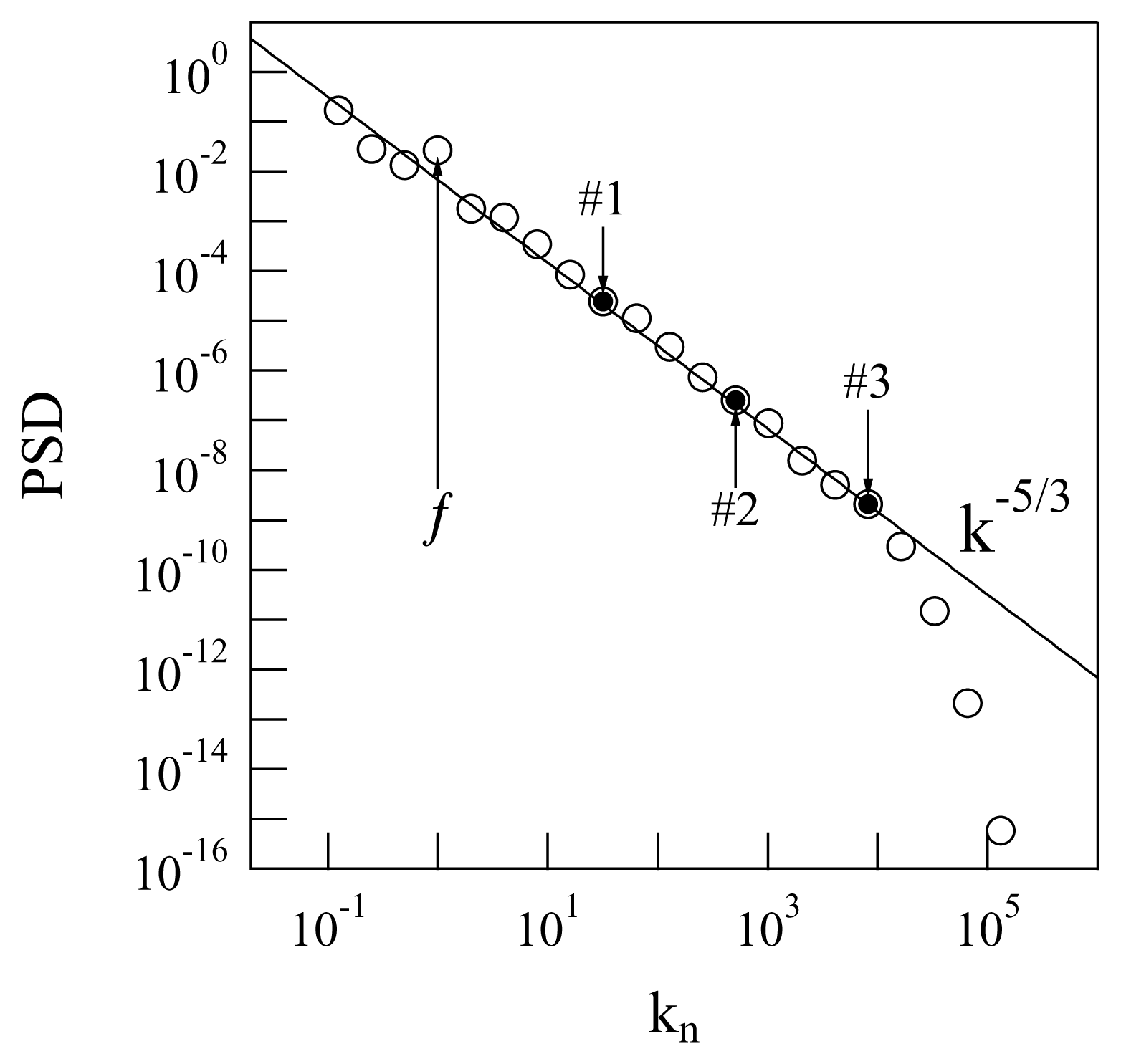
The stirring force pumps energy and momentum into the fluid, injecting them at the fourth scale, and the energy and momentum are transferred from u4 to all the other modes via the non-linear couplings. There is a scale for each kn and eddy turnover time τn. At each kn, a corresponds. The characteristic times of the system will be naturally assigned in terms of the zeroth mode eddy turnover time, τ0, or of other τns. After a certain transitory regime, the system reaches an “equilibrium” from the time-average point of view, in which the Fourier spectrum appears for the classical energy cascade of turbulence, as predicted by Kolmogorov [29] (see Figure 1).
The quantity represented along the ordinate axis of Figure 1 is the average power spectral density (PSD), defined as follows:
where [t1, t2] is a time-interval taken after a sufficiently long time, such that the system (14) has already reached its stationary regime (i.e., after some initial transient regime with heterogeneous fluctuations in which the turbulence is not fully developed yet). The evaluation of the duration of the transient regime is made “glancing at” the development of the plot of versus kn as the simulation time runs and picking the moment after which this plot does not change any more. In terms of the quantities involved in Equation (15), this means t1 is “many times” the largest eddy turnover time.
The energetic, and informatic, behavior of the GOY system is critically influenced by the form of the dissipative term, , in Equation (14): the presence of the factor, , implies that the energy loss is more and more important for higher and higher |kn|, i.e., smaller and smaller scales. The energy flows from any mode, un, both towards the smaller and the higher scales, since un is coupled both with the smaller scales and larger scales. Energy is dissipated at all the scales, but the dissipation efficiency grows with , so that almost no net energy can really reflow back from the small scales to the large ones. In terms of cross-predictability, a pass of information in both verses is expected, but the direct cascade (i.e., from small to large |kn|s) should be prevalent. Not only this: since the ordinary differential equations Equation (14) indicate a k-local interaction (up to the second-adjacent n, i.e., n ± 1 and n ± 2 coupling with n), one also expects the coupling between um and un≫m or un≪m to be almost vanishing and the characteristic interaction times to be shorter for closer values of m and n. Our program is to check all these expectations by calculating the transfer entropy and its normalized version for the synthetic data obtained running the GOY model (14). In particular, we would like to detect the verse of information transfer along the inertial domain between shells not directly coupled in the evolution Equation (14).
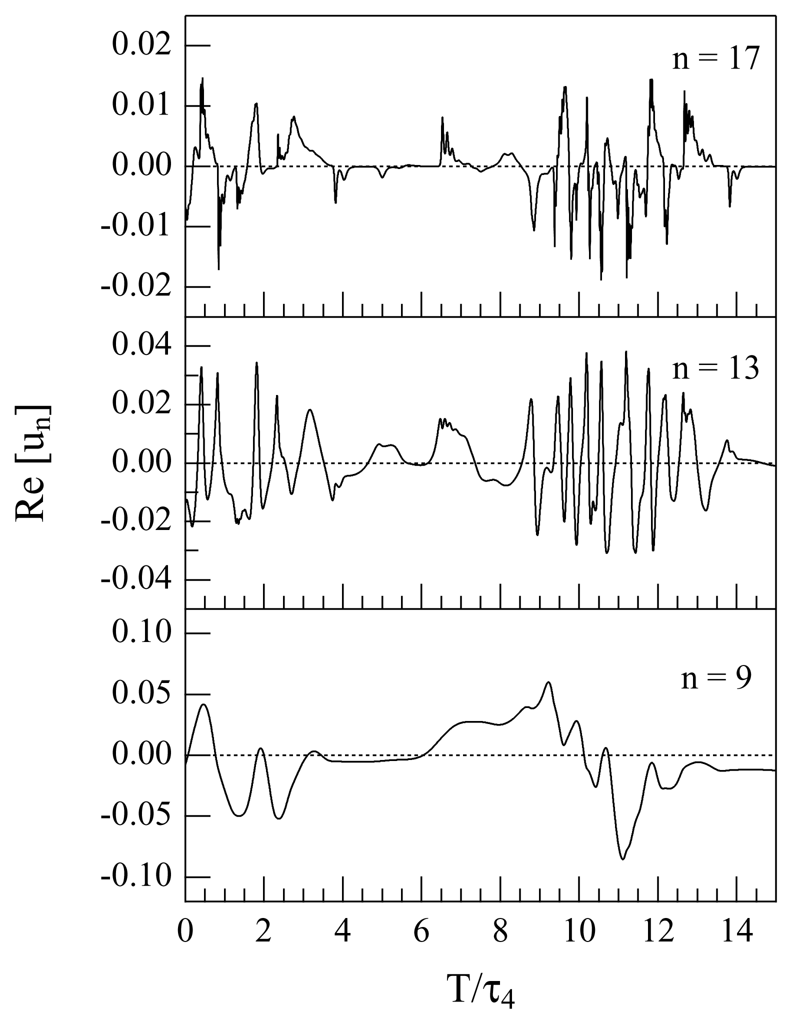
To get the above target, and to investigate the application of TEA to the GOY model and illustrate the advantages of using the new normalized quantities discussed in Section 2, we selected three non-consecutive shells. In particular, the choice:
is made. The real parts of u9, u13 and u17 are reported in Figure 2 as functions of time for a short time interval of 15 τ4. For each of the selected shells, we considered very long time series of the corresponding energy en = |un|2. The typical length of the considered time series is of many (≃ 1, 000) eddy turnover times of the injection scale.
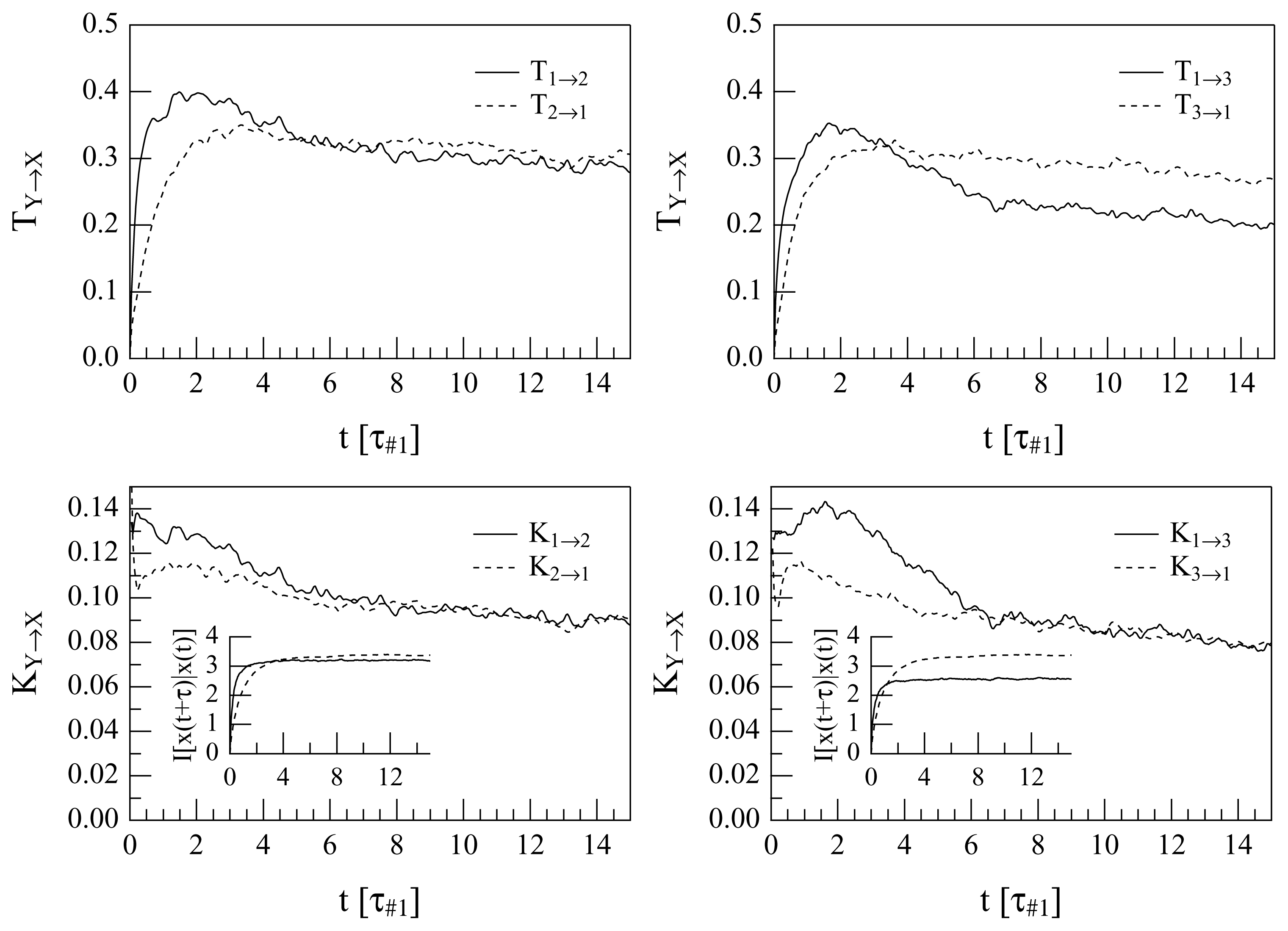
The quantities, ΔT1→2 and ΔT1→3, and ΔK1→2 and ΔK1→3, can be calculated as functions of the delay, τ. The difference ΔTi→j or ΔKi→j are calculated as prescribed in Section 2 using the time series, ei (t) and ej (t), in the place of y (t) and x (t), respectively. The calculations of the quantities, T1→2, T2→1, T1→3, T3→1 and the corresponding quantities normalized, i.e., K1→2, K2→1, K1→3 and K3→1, give the results portrayed in Figure 3, where all these quantities are reported synoptically as a function of τ in units of the eddy turnover time, τ#1, that pertains to the 1 mode (with n = 9).
The use of non-adjacent shells to calculate the transfer of information is a choice: the interaction between nearby shells is obvious from Equation (14), while checking the existence of an information transfer cascade down from the large to the small scales requires checking it non-locally in the k-space.
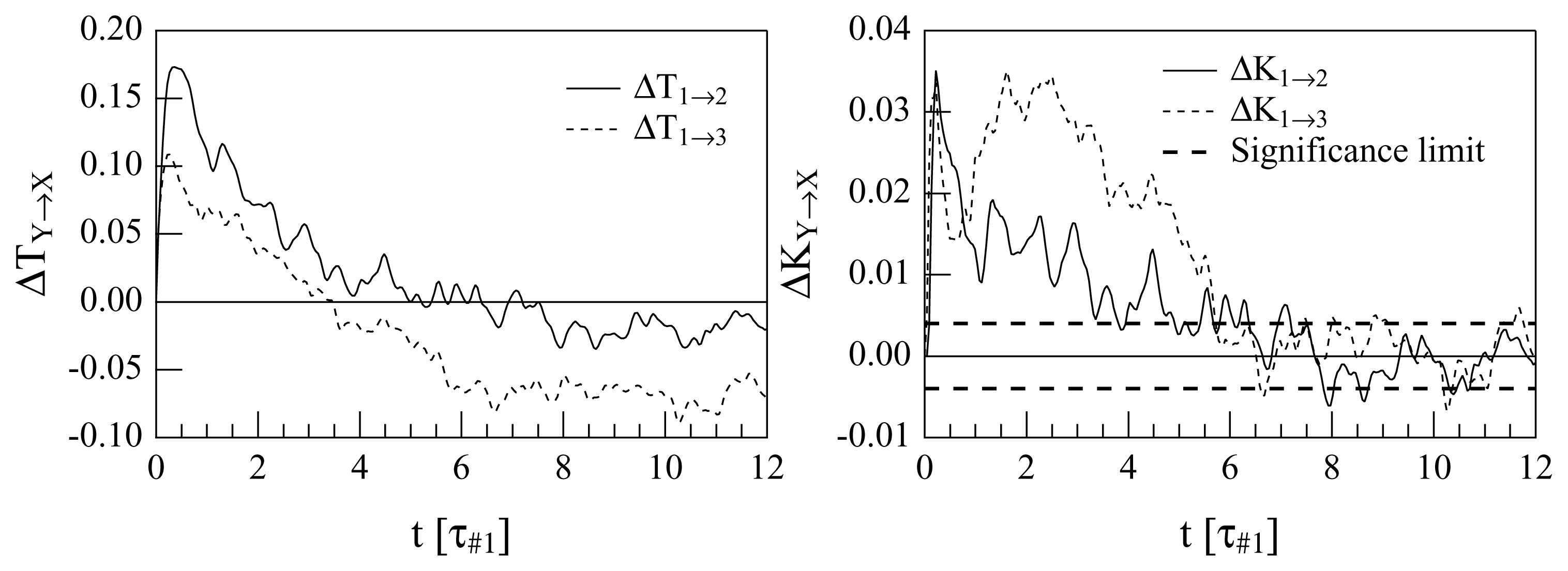
All the plots show clearly that there is a direct cascade for short delays. The first noticeable difference between the transfer entropies and the normalized transfer entropies is that in the #1 ↔ #3 coupling, a non-understandable inverse regime appears after about 4τ#1, when the “traditional” transfer entropy is used. Instead, the use of the normalized quantities suggests decoupling after long times (after about 6τ#1). A comparison between the #1 ↔ #2 and #1 ↔ #3 interactions is also interesting: the maximum of the “direct cascade” coupling is reached at less than 0.5τ#1 for both the interactions if the TEs are used. However in the plot of K1→2, K2→1, K1→3 and K3→1, some time differences appear; this is clarified when difference quantities are plotted, as in Figure 4.
Both the analyses diagnose a prevalence of the smaller-onto-larger wavenumber drive for sufficiently small delays: the ΔT1→2 indicates a driving of u9 onto u13 (Mode #1 onto Mode #2) for τ ≲ 5τ#1, while ΔT1→3 indicates a driving of u9 onto u17 (Mode #1 onto Mode #3) for τ ≲ 3.5τ#1. This is expected, due to how the system (14) is constructed. What is less understandable is the fact that for large values of τ, the quantities ΔT1→2 (τ ) and, even more, ΔT1→3 (τ ) become negative. This would suggest that after a long time a (weaker) “inverse cascade” prevails; however, this is not contained in the system (14) in any way and, hence, is either evidence of chaos-driven unpredictability or is an erroneous interpretation. For this reason, it is instructive to examine the plots of Δ1→2K (τ ) and Δ1→3K (τ ): after roughly 6.5τ#1, the modes appear to become decoupled, since Δ1→2K ≃ 0 and Δ1→3K ≃ 0, albeit with significant noise. The lack of evidence of an inverse cascade in these plots suggests that the interpretation of an inverse cascade as descending from the old TEA was wrong.
The misleading response of the ΔT analysis may be well explained looking at the insets in the lower plots of Figure 3, where the quantities reported as functions of τ are the normalization coefficients, It (Xτ |X), indicating the levels of inherent unpredictability of the two en (t) compared. In the case of the 1 → 2 comparison, the levels of inherent unpredictability of the two time series, e9 (t) and e13 (t), become rather similar for large τ, while the asymptotic levels of inherent unpredictability are very different for e9 (t) and e17 (t) (indeed, one should expect that the more different is m from n, the more different level of inherent unpredictability will be shown by em and en). This means that ΔT1→2 (τ ) and Δ1→2K (τ ) are expected to give a rather similar diagnosis, while the calculation of Δ1→3K (τ ) will probably fix any misleading indication of ΔT1→3 (τ ).
Another observation that deserves to be made is about the maxima of ΔT1→2 (τ ), ΔT1→3 (τ ), Δ1→2K (τ ) and Δ1→3K (τ ) with respect to τ : this should detect the characteristic interaction time for the interaction, (e9, e13), and for the interaction, (e9, e17). In the plots of ΔT1→2 (τ ) and ΔT1→3 (τ ), one observes a maximum for ΔT1→2 at τ ≃ 0.6τ#1 and a maximum for ΔT1→3 just slightly before this. It appears that the characteristic time of interaction of e9 with e13 is slightly larger than of e9 with e17: this is a little bit contradictory, because of the k-local hypothesis after which the energy is transferred from e9 to e13 and then to e17.
What happens in the plots of Δ1→2K (τ ) and Δ1→3K (τ ) is different and more consistent with what we know about the GOY model. First of all, the maximum for Δ1→3K is not unique: there is a sharp maximum at about 0.5τ#1, which comes a little bit before the maximum of Δ1→2K, exactly as in the case of the ΔTs. However, now, the big maxima of Δ1→3K are occurring between 1.5 and 3 times τ#1, so that maybe different processes in the interaction, (e9, e17), are emerging. Actually, distant wavenumbers may interact through several channels, and more indirect channels enter the play as the wavenumbers become more distant. This might explain the existence de facto of two different characteristic times for the interaction, (e9, e17), as indicated by the plot of ΔK1→3 (τ ): a very early one at about 0.5τ#1; and a later one within the interval (1.5τ#1, 3.5τ#1).
The differences between the TEAs performed with ΔT and ΔK appear to be better understandable considering that through the normalization in ΔK, one takes into account the self information entropy of each process (i.e., the degree of unpredictability of each process). The motivation is essentially identical to the preference of relative error over absolute error in many applications.
As far as the surrogate data test used to produce the level of confidence in Figure 4, we use the method described in [33]. In this case, a set of more than 104 surrogate data copies have been realized, by randomizing the Fourier phases. In each of these surrogate datasets, the delayed transfer entropy was calculated. Than, a statistical analysis, with a confidence threshold of five percent, was performed. A similar level of confidence was obtained also for the results in Figure 3, but it is not reported explicitly on the plot for clarity.
4. Conclusions
Mutual information and transfer entropy are increasingly used to discern whether relationships exist between variables describing interacting processes, and if so, what is the dominant direction of dynamical influence in those relationships? In this paper, these IDQs are normalized in order to account for potential differences in the intrinsic stochasticity of the coupled processes.
A process, Y, is considered to influence a process, X, if their interaction reduces the unpredictability of X: this is why one chooses to normalize the IDQs with respect to the Shannon entropy of X, taken as a measure of its unpredictability.
The normalized transfer entropy is particularly promising, as has been illustrated for a synthetic model of fluid turbulence, namely the GOY model. The results obtained here about the transfer entropy and its normalized version for the interactions between Fourier modes of this model point towards the following conclusions.
The fundamental characteristics of the GOY model non-linear interactions, expected by construction, are essentially re-discovered via the TEA of its Fourier components, both using the unnormalized IDQs and the normalized ones: the prevalence of the large-to-small scale cascade; the locality of the interactions in the k-space; the asymptotic decoupling after a suitably long delay. The determination of the correct verse of dynamical enslaving is better visible using KY→X and ΔKY→X, in which the intrinsic randomness of the two processes is taken into account (in particular, the inspection of ΔTY→X indicated the appearance of an unreasonable inverse cascade for large τ, which was ruled out by looking at ΔKY→X).
An indication is then obtained that for the irregular non-linear dynamics at hand, the use of the TEA via ΔKY→X (τ ; t) is promising in order to single out relationships of cross-predictability (transfer of information) between processes.
The systematic application of the TEA via ΔKY→X to models and natural systems is going to be done in the authors’ forthcoming works.
Conflicts of Interest
The authors declare no conflict of interest.
References
- Shannon, C.E. A mathematical theory of communication. Bell Syst. Tech. J 1948, 27. [Google Scholar]
- A Good Introduction on SDSs May Be Found in the Webiste. Available online: http://www.scholarpedia.org/article/Stochastic_dynamical_systems accessed on 16 July 2013.
- Klimontovich, Y.L. Statistical Theory of Open Systems; Kluwer Academic Publishers: Dordrecht, The Netherlands, 1995; Volume 1. [Google Scholar]
- Elskens, Y.; Prigogine, I. From instability to irreversibility. Proc. Natl. Acad. Sci. USA 1986, 83, 5756–5760. [Google Scholar]
- Kullback, S. Information Theory and Statistics; Wiley: New York, NY, USA, 1959. [Google Scholar]
- Kantz, H.; Schreiber, T. Nonlinear Time Series Analysis; Cambridge University Press: Cambridge, MA, USA, 1997. [Google Scholar]
- Schreiber, T. Measuring information transfer. Phys. Rev. Lett 2000, 85, 461–464. [Google Scholar]
- Hlaváčková-Schindler, K.; Paluš, M.; Vejmelkab, M.; Bhattacharya, J. Causality detection based on information-theoretic approaches in time series analysis. Phys. Rep 2007, 441, 1–46. [Google Scholar]
- Materassi, M.; Wernik, A.; Yordanova, E. Determining the verse of magnetic turbulent cascades in the Earth’s magnetospheric cusp via transfer entropy analysis: Preliminary results. Nonlinear Processes Geophys 2007, 14, 153–161. [Google Scholar]
- De Michelis, P.; Consolini, G.; Materassi, M.; Tozzi, R. An information theory approach to storm-substorm relationship. J. Geophys. Res 2011. [Google Scholar] [CrossRef]
- Bauer, M.; Thornhill, N.F.; Meaburn, A. Specifying the directionality of fault propagation paths using transfer entropy. Proceedings of the 7th International Symposium on Dynamics and Control of Process Systems, Cambridge, MA, USA,, 5–7 July 2004.
- Kaiser, A.; Schreiber, T. Information transfer in continuous processes. Phys. D 2002, 166, 43–62. [Google Scholar]
- Kwon, O.; Yang, J.-S. Information flow between stock indices. Eur. Phys. Lett 2008. [Google Scholar] [CrossRef]
- Kugiumtzis, D. Improvement of Symbolic Transfer Entropy. Proceedings of the 3rd International Conference on Complex Systems and Applications, Normandy, France, 29 June – 2 July 2009; pp. 338–342.
- Tung, T.Q.; Ryu, T.; Lee, K.H.; Lee, D. Inferring Gene Regulatory Networks from Microarray Time Series Data Using Transfer Entropy. Proceedings of the Twentieth IEEE International Symposium on Computer-Based Medical Systems (CBMS’07), Maribor, Slovenia, 20–22 June 2007.
- Kleeman, R. Measuring dynamical prediction utility using relative entropy. J. Atmos. Sci 2002, 59, 2057–2072. [Google Scholar]
- Kleeman, R. Information flow in ensemble weather oredictions. J. Atmos. Sci 2007, 64, 1005–1016. [Google Scholar]
- Vicente, R.; Wibral, M.; Lindner, M.; Pipa, G. Transfer entropy—A model-free measure of effective connectivity for the neurosciences. J. Comput. Neurosci 2011, 30, 45–67. [Google Scholar]
- Lizier, J.T.; Heinzle, J.; Horstmann, A.; Haynes, J.-D.; Prokopenko, M. Multivariate information-theoretic measures reveal directed information structure and task relevant changes in fMRI connectivity. J. Comput. Neurosci 2011, 30, 85–107. [Google Scholar]
- Jaynes, E.T. Information theory and statistical mechanics. Phys. Rev 1957, 106, 620–630. [Google Scholar]
- Lizier, J.T. The Local Information Dynamics of Distributed Computation in Complex Systems. Ph.D. Thesis, The University of Sydney, Darlington, NSW, Australia, 11 October 2010. [Google Scholar]
- Papana, A.; Kugiumtzis, D. Reducing the bias of causality measures. Phys. Rev. E 2011, 83, 036207. [Google Scholar]
- Faes, L.; Nollo, G.; Porta, A. Information-based detection of nonlinear Granger causality in multivariate processes via a nonuniform embedding technique. Phys. Rev. E 2011, 83, 051112. [Google Scholar]
- Materassi, M.; Ciraolo, L.; Consolini, G.; Smith, N. Predictive Space Weather: An information theory approach. Adv. Space Res 2011, 47, 877–885. [Google Scholar]
- Wibral, M.; Pampu, N.; Priesmann, V.; Siebenhühner, F.; Seiwart, H.; Lindner, M.; Lizier, J.T.; Vincente, R. Measuring information-transfer delays. PLoS One 2013, 8, e55809. [Google Scholar]
- Phythian, R. The functional formalism of classical statistical dynamics. J. Phys. A 1977, 10, 777–789. [Google Scholar]
- Bar-Yam, Y. A mathematical theory of strong emergence using mutiscale variety. Complexity 2009, 9, 15–24. [Google Scholar]
- Ryan, A.J. Emergence is coupled to scope, not level. Complexity 2007, 13, 67–77. [Google Scholar]
- Frisch, U. Turbulence, the Legacy of A. N. Kolmogorov; Cambridge University Press: Cambridge, UK, 1995. [Google Scholar]
- Ditlevsen, P.D. Turbulence and Shell Models; Cambridge University Press: Cambridge, UK, 2011. [Google Scholar]
- Knuth, K.H. Optimal data-based binning for histograms 2006. arXiv:physics/0605197 v1.
- Pisarenko, D.; Biferale, L.; Courvoisier, D.; Frisch, U.; Vergassola, M. Further results on multifractality in shell models. Phys. Fluids A 1993, 5, 2533–2538. [Google Scholar]
- Theiler, J.; Eubank, S.; Longtin, A.; Galdrikian, B.; Doyne Farmer, J. Testing for nonlinearity in time series: The method of surrogate data. Phys. D 1992, 58, 77–94. [Google Scholar]


© 2014 by the authors; licensee MDPI, Basel, Switzerland This article is an open access article distributed under the terms and conditions of the Creative Commons Attribution license (http://creativecommons.org/licenses/by/3.0/).
Share and Cite
Materassi, M.; Consolini, G.; Smith, N.; De Marco, R. Information Theory Analysis of Cascading Process in a Synthetic Model of Fluid Turbulence. Entropy 2014, 16, 1272-1286. https://doi.org/10.3390/e16031272
Materassi M, Consolini G, Smith N, De Marco R. Information Theory Analysis of Cascading Process in a Synthetic Model of Fluid Turbulence. Entropy. 2014; 16(3):1272-1286. https://doi.org/10.3390/e16031272
Chicago/Turabian StyleMaterassi, Massimo, Giuseppe Consolini, Nathan Smith, and Rossana De Marco. 2014. "Information Theory Analysis of Cascading Process in a Synthetic Model of Fluid Turbulence" Entropy 16, no. 3: 1272-1286. https://doi.org/10.3390/e16031272