Infinite Excess Entropy Processes with Countable-State Generators


Abstract
: We present two examples of finite-alphabet, infinite excess entropy processes generated by stationary hidden Markov models (HMMs) with countable state sets. The first, simpler example is not ergodic, but the second is. These are the first explicit constructions of processes of this type.PACS Classification: 02.50.-r 89.70.+c 05.45.Tp 02.50.Ey1. Introduction
For a stationary process (Xt) the excess entropy E is the mutual information between the infinite past X⃖ = . . . X−2X−1 and the infinite future X⃗ = X0X1 . . .. It has a long history and is widely employed as a measure of correlation and complexity in a variety of fields, from ergodic theory and dynamical systems to neuroscience and linguistics [1–6]. For a review the reader is referred to [7].
An important question in classifying a given process is whether the excess entropy is finite or infinite. In the former case the process is said to be finitary, and in the latter infinitary.
Over a finite alphabet, most of the commonly studied, simple process types are always finitary, including all independent identically distributed (IID) processes, finite-order Markov processes, and processes with finite-state hidden Markov model (HMM) presentations. However, there are also well known examples of finite-alphabet, infinitary processes. For instance, the symbolic dynamics at the onset of chaos in the logistic map and similar dynamical systems [7] and the stationary representation of the binary Fibonacci sequence [8] are both infinitary.
These latter processes, though, only admit stationary HMM presentations with uncountable state sets. Indeed, one can show that any process generated by a stationary, countable-state HMM either has positive entropy rate or consists entirely of periodic sequences, which these do not. Versions of the Santa Fe Process introduced in [6] are finite-alphabet, infinitary processes with positive entropy rate. However, they were not constructed directly as hidden Markov processes, and it seems unlikely that they should have any stationary, countable-state presentations either.
Here, we present two examples of stationary, countable-state HMMs that do generate finite-alphabet, infinitary processes. To the best of our knowledge, these are the first explicit constructions of this type in the literature. Although, subsequent to our release of the earlier version of the present work [9], two additional examples were given in [10].
Our first example is nonergodic, and the information conveyed from the past to the future essentially consists of the ergodic component along a given realization. This example is straightforward to construct and, though previously unpublished, others are likely aware of it or similar constructions. The second, ergodic example, though, is more involved, and both its structure and properties are novel.
To put these contributions in perspective, we note that any stationary, finite-alphabet process may be trivially presented by a stationary hidden Markov model with an uncountable state set, in which each infinite history ⃖ corresponds to a single state. Thus, it is clear that stationary HMMs with uncountable state sets can generate finite-alphabet, infinitary processes. In contrast, for any finite-state HMM E is always finite—bounded by the logarithm of the number of states. The case of countable-state HMMs lies in-between the finite-state and uncountable-state cases, and it was previously not demonstrated whether it is possible to have countable-state, stationary HMMs that generate infinitary, finite-alphabet processes and, in particular, ergodic ones.
2. Background
2.1. Excess Entropy
We denote by H [X] the Shannon entropy in a random variable X, by H [X|Y ] the conditional entropy in X given Y, and by I [X; Y ] the mutual information between random variables X and Y. For definitions of these information theoretic quantities, as well as the definitions of stationarity and ergodicity for a stochastic process (Xt), the reader is referred to [11].
Definition 1
For a stationary, finite-alphabet process (Xt)t∈ℤ the excess entropy E is the mutual information between the infinite past X⃖ = . . . X−2X−1 and the infinite future X⃗ = X0X1 . . . :
where X⃖t = X−t . . . X−1 and X⃗t = X0 . . . Xt−1 are the length-t past and future, respectively.
As noted in [7,12] this quantity, E, may also be expressed alternatively as:
where h is the process entropy rate:
That is, the excess entropy E is the asymptotic amount of entropy (information) in length-t blocks of random variables beyond that explained by the entropy rate. The excess entropy derives its name from this latter formulation. It is also this formulation that we use to establish that the process of Section 3.1 is infinitary.
Expanding the block entropy H [X⃗t] in Equation (2) with the chain rule and recombining terms gives another important formulation [7]:
where h(t) is the length-t entropy-rate approximation:
the conditional entropy in the t-th symbol given the previous t – 1 symbols. This final formulation will be used to establish that the process of Section 3.2 is infinitary.
2.2. Hidden Markov Models
There are two primary types of hidden Markov models: edge-emitting (or Mealy) and state-emitting (or Moore). We work with the former edge-emitting type, but the two are equivalent in that any model of one type with a finite output alphabet may be converted to a model of the other type without changing the cardinality of the state set by more than a constant factor—the alphabet size. Thus, for our purposes, Mealy HMMs are sufficiently general. We also consider only stationary HMMs with finite output alphabets and countable state sets.
Definition 2
A stationary, edge-emitting, countable-state, finite-alphabet hidden Markov model (hereafter referred to simply as a countable-state HMM) is a 4-tuple (
 ,
,  , {T(x)}, π) where:
- (1)
![Entropy 16 01396f4]() is a countable set of states.
is a countable set of states.- (2)
![Entropy 16 01396f5]() is a finite alphabet of output symbols.
is a finite alphabet of output symbols.- (3)
T(x), x ∈
![Entropy 16 01396f5]() , are symbol labeled transition matrices whose sum T = ∑x∈
, are symbol labeled transition matrices whose sum T = ∑x∈
![Entropy 16 01396f5]() T(x) is stochastic. is the probability that state σ transitions to state σ′ on symbol x.
T(x) is stochastic. is the probability that state σ transitions to state σ′ on symbol x.- (4)
π is a stationary distribution for the underlying Markov chain over states with transition matrix T. That is, π satisfies π = πT.
Remarks
- (1)
“Countable” in Property 1 means either finite or countably infinite. If the state set
![Entropy 16 01396f4]() is finite, we also refer to the HMM as finite-state.
is finite, we also refer to the HMM as finite-state.- (2)
We do not assume, in general, that the underlying Markov chain over states with transition matrix T is irreducible. Thus, even in the case that
![Entropy 16 01396f4]() is finite, the stationary distribution π is not necessarily uniquely defined by the matrix T and is, therefore, specified separately.
is finite, the stationary distribution π is not necessarily uniquely defined by the matrix T and is, therefore, specified separately.
Visually, a hidden Markov model may be depicted as a directed graph with labeled edges. The vertices are the states σ ∈
and, for all σ, σ′ ∈
with
, there is a directed edge from state σ to state σ′ labeled p|x for the symbol x and transition probability
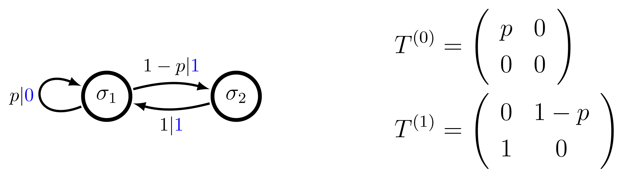
. These probabilities are normalized so that the sum of probabilities on all outgoing edges from each state is 1. An example is given in Figure 1.
The operation of a HMM may be thought of as a weighted random walk on the associated graph. From the current state σ the next state σ′ is determined by following an outgoing edge from σ chosen according to the edge probabilities (or weights). During the transition, the HMM also outputs the symbol x labeling this edge.
We denote the state at time t by St and the t-th symbol by Xt, so that symbol Xt is generated upon the transition from state St to state St+1. The state sequence (St) is simply a Markov chain with transition matrix T. However, we are interested not simply in this sequence of states, but also in the associated sequence of output symbols (Xt) that are generated by reading the labels off the edges as they are followed. The interpretation is that an observer of the HMM may directly observe this sequence of output symbols, but not the hidden internal states. Alternatively, one may consider the Markov chain over edges (Et), of which the observed symbol sequence (Xt) is simply a projection.
In either case, the process (Xt) generated by the HMM (
, , {T(x)}, π) is defined as the output sequence of edge symbols, which results from running the Markov chain over states according to the stationary law with marginals ℙ(S0) = ℙ(St) = π. It is easy to verify that this process is itself stationary, with word probabilities given by:
where for a given word w = w1...wn ∈
*, T(w) is the word transition matrix T(w) = T(w1) · · · T(wn).
Remark
Even for a nonstationary HMM (
, , {T(x)}, ρ), where the state distribution ρ is not stationary, one may always define a one-sided process (Xt)t≥0 with marginals given by:
Furthermore, though the state sequence (St)t≥0 will not be a stationary process if ρ is not a stationary distribution for T, the output sequence (Xt)t≥0 may still be stationary. In fact, as shown in [12] (Example 2.9), any one-sided process over a finite alphabet , stationary or not, may be represented by a countable-state, nonstationary HMM in which the states correspond to finite-length words in *, of which there are only countably many. By stationarity, a one-sided stationary process generated by such a nonstationary HMM can be uniquely extended to a two-sided stationary process. So, in a sense, any two-sided stationary process (Xt)t∈ℤ can be said to be generated by a nonstationary, countable-state HMM. Though, this is a slightly unnatural interpretation of process generation in that the two-sided process (Xt)t∈ℤ is not directly that obtained by reading symbols off the edges of the HMM as it runs along transitioning between states in bi-infinite time. In either case, the space of stationary, finite-alphabet processes generated by nonstationary, countable-state HMMs is too large: it includes all stationary, finite-alphabet processes. Due to this, we restrict to the case of stationary HMMs where both the state sequence (St) and output sequence (Xt) are stationary processes, and henceforth use the term HMM implicitly to mean stationary HMM. Clearly, if one allows finite-alphabet processes generated by nonstationary, countable-state HMMs there are infinitary examples.
We consider now an important property known as unifilarity. This property is useful in that many quantities are analytically computable only for unifilar HMMs. In particular, for unifilar HMMs the entropy rate h is often directly computable, unlike in the nonunifilar case. Both of the examples constructed in Section 3 are unifilar, as is the Even Process HMM of Figure 1.
Definition 3
A HMM (
, , {T(x)}, π) is unifilar if for each σ ∈
and x ∈
there is at most one outgoing edge from state σ labeled with symbol x in the associated graph G.
It is well known that for any finite-state, unifilar HMM the entropy rate in the output process (Xt) is simply the conditional entropy in the next symbol given the current state:
where πσ is the stationary probability of state σ and hσ = H [X0|S0 = σ] is the conditional entropy in the next symbol given that the current state is σ.
We are unaware, though, of any proof that this is generally true for countable-state HMMs. If the entropy in the stationary distribution H [π] is finite, then a proof along the lines given in [13] carries through to the countable-state case and Equation (8) still holds. However, countable-state HMMs may sometimes have H [π] = ∞. Furthermore, it can be shown [12] that the excess entropy E is always bounded above by H [π]. So, for the infinitary process of Section 3.2 we need slightly more than unifilarity to establish the value of h. To this end, we consider a property known as exactness [14].
Definition 4
A HMM is said to be exact if for a.e. infinite future ⃗ = x0x1... generated by the HMM an observer synchronizes to the internal state after a finite time. That is, for a.e. ⃗ there exists t ∈ ℕ such that H [St|X⃗t = ⃗⃗ t] = 0, where ⃗t = x0x1...xt−1 denotes the the first t symbols of a given ⃗.
In the appendix we prove the following proposition.
Proposition 1
For any countable-state, exact, unifilar HMM the entropy rate is given by the standard formula of Equation (8).
The HMM constructed in Section 3.2 is both exact and unifilar, so Proposition 1 applies. Using this explicit formula for h, we will show that is infinite.
3. Constructions
We now present the two constructions of (stationary) countable-state HMMs that generate infinitary processes. In the first example the output process is not ergodic, but in the second it is.
3.1. Heavy-Tailed Periodic Mixture: An infinitary nonergodic process with a countable-state presentation
Figure 2 depicts a countable-state HMM M, for a nonergodic infinitary process ℘. The machine M consists of a countable collection of disjoint strongly connected subcomponents Mi, i ≥ 2. For each i, the component Mi generates the periodic process ℘i consisting of i – 1 1s followed by a 0. The weighting (μ2, μ3, ..., ) over components is taken as a heavy-tailed distribution with infinite entropy. For this reason, we refer to the process M generates as the Heavy-Tailed Periodic Mixture (HPM) process.
Intuitively, the information transmitted from the past to the future for the HPM Process is the ergodic component i along with the phase of the period-i process ℘i in this component. This is more information than simply the ergodic component i, which is itself an infinite amount of information: H [(μ2, μ3, ..., )] = ∞. Hence, E should be infinite. This intuition can be made precise using the ergodic decomposition theorem of Debowski [15], but we present a more direct proof here.
Proposition 2
The HPM Process has infinite excess entropy.
Proof
For the HPM Process ℘ we will show that (i) limt→∞ H [X⃗t] = ∞and (ii) h = 0. The conclusion then follows immediately from Equation (2). To this end, we define sets:
Note that any word w ∈ Wi,t with i ≤ t/2 contains at least two 0s. Therefore:
- (1)
No two distinct states σij and σij′ with i ≤ t/2 generate the same length t word.
- (2)
The sets Wi,t, i ≤ t/2, are disjoint from both each other and Vt.
It follows that each word w ∈ Wi,t, with i ≤ t/2, can only be generated from a single state σij of the HMM and has probability:
Hence, for any fixed t:
so:
which proves Claim (i). Now, to prove Claim (ii) consider the quantity:
On the one hand, for w ∈ Ut, H [Xt|X⃗t = w] = 0 since the current state and, hence, entire future are completely determined by any word w ∈ Ut. On the other hand, for w ∈ Vt, H [Xt|X⃗t = w] ≤ 1 since the alphabet is binary. Moreover, the combined probability of all words in the set Vt is simply the probability of starting in some component Mi with i > t/2: ℙ(Vt) = ∑i>t/2 μi. Thus, by Equation (11)h(t + 1) ≤ ∑ i>t/2 μi. Since ∑i μi converges, it follows that h(t) ↘ 0, which verifies Claim (ii).
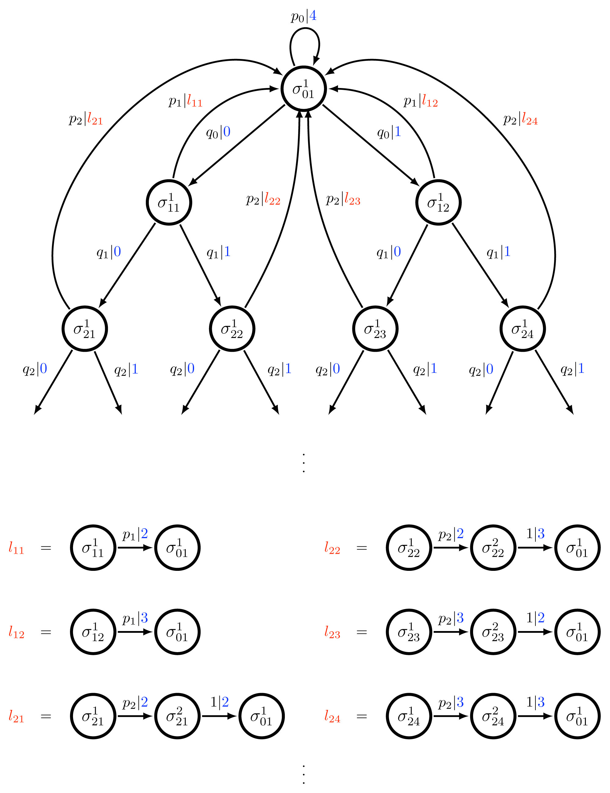
3.2. Branching Copy Process: An infinitary ergodic process with a countable-state presentation
Figure 3 depicts a countable-state HMM M for the ergodic, infinitary Branching Copy Process. Essentially, the machine M consists of a binary tree with loop backs to the root node. From the root a path is chosen down the tree with each left-right (or 0–1) choice equally likely. But, at each step there is also a chance of turning back towards the root. The path back is a not a single step, however. It has length equal to the number of steps taken down the tree before returning back, and copies the path taken down symbol-wise with 0 s replaced by 2 s and 1 s replaced by 3 s. There is also a high self-loop probability at the root node on symbol 4, so some number of 4 s will normally be generated after returning to the root node before preceding again down the tree. The process generated by this machine is referred to as the Branching Copy (BC) Process, because the branch taken down the tree is copied on the loop back to the root.
By inspection we see that the machine is unifilar with synchronizing word w = 4, i.e., H [S1|X0 = 4] = 0. Since the underlying Markov chain over states (St) is positive recurrent, the state sequence (St) and symbol sequence (Xt) are both ergodic. Thus, a.e. infinite future ⃗ contains a 4, so the machine is exact. Therefore, Proposition 1 may be applied, and we know the entropy rate h is given by the standard formula of Equation (8): h = ∑σ πσhσ. Since ℙ(St = σ) = πσ for any t ∈ ℕ, we may alternatively represent this entropy rate as:
where t = {w : |w| = t, ℙ(w) > 0} is the set of length t words in the process language , φ(w) is the conditional state distribution induced by the word w (i.e., φ(w)σ = ℙ(St = σ|X⃗t = w)), and h̃w = ∑σ φ(w)σhσ is the φ(w)-weighted average entropy in the next symbol given knowledge of the current state σ. Similarly, for any t ∈ ℕ the entropy-rate approximation h(t + 1) may be expressed as:
where hw = H [Xt|X⃗t = w] is the entropy in the next symbol after observing the word w. Combining Equations (12) and (13) we have for any t ∈ ℕ:
As we will show in Claim 6, concavity of the entropy function implies the quantity hw – h̃w is always nonnegative. Furthermore, in Claim 5 we will show that hw–h̃w is always bounded below by some fixed positive constant for any word w consisting entirely of 2s and 3s. Also, in Claim 3 we will show that ℙ(Wt) scales as 1/t, where Wt is the set of length-t words consisting entirely of 2s and 3s. Combining these results it follows that h(t + 1) – h ≥̃ 1/t and, hence, the sum is infinite.
A more detailed analysis with the claims and their proofs is given below. In this we will use the following notation:
ℙσ(·) = ℙ(·|S0 = σ),
Vt = {w ∈ t : w contains only 0s and 1s} and Wt = {w ∈ t : w contains only 2s and 3s},
is the stationary probability of state ,
, and
and .
Note that:
and:
These facts will be used in the proof of Claim 1.
Claim 1
The underlying Markov chain over states for the HMM is positive recurrent.
Proof
Let be the first return time to state . Then, by continuity:
Hence, the Markov chain is recurrent and we have:
from which it follows that the chain is also positive recurrent. Note that the topology of the chain implies the first return time may not be an odd integer greater than 1.
Claim 2
The stationary distribution π has:
where.
Proof
Existence of a unique stationary distribution π is guaranteed by Claim 1. Given this, clearly . Similarly, for i ≥ 1, , from which it follows by induction that , for all i ≥ 1. By symmetry for each i ∈ ℕ and 1 ≤ j ≤ 2i. Therefore, for each i ∈ ℕ, 1 ≤ j ≤ 2i we have as was claimed. Moreover, for i ≥ 2, . Combining with the expression for gives . By induction, , so this completes the proof.
Note that for all i ≥ 1 and 1 ≤ j ≤ 2i:
Also note that for any t ∈ ℕ and i ≥ 2t we have for each 1 ≤ j ≤ 2i:
- (1)
, for 2 ≤ k ≤ ⌈i/2⌉ + 1.
- (2)
and . Hence, .
Therefore, for each t ∈ ℕ:
Equations (19), (20), and (21) will be used in the proof of Claim 3 below, along with the following simple lemma.
Lemma 1 (Integral Test)
Let n ∈ ℕ and let f : [n,∞] → ℝ be a positive, continuous, monotone-decreasing function, then:
Claim 3
ℙ(Wt) decays roughly as 1/t. More exactly, C/12t ≤ ℙ(Wt) ≤ 6C/t for all t ∈ ℕ.
Proof
For any state with i < t, . Thus, we have:
where the final equality follows from symmetry. We prove the bounds from above and below on ℙ(Wt) separately using Equation (22).
Bound from below:
Here, (a) follows from Equations (19) and (21) and (b) from Lemma 1.
Bound from above:
Here, (a) follows from Equation (20) and (b) from Lemma 1.
Claim 4
ℙ(Xt ∈ {2, 3}|X⃗t = w) ≥ 1/150, for all t ∈ ℕ and w ∈ Wt.
Proof
Applying Claim 3 we have for any t ∈ ℕ:
By symmetry, ℙ(Xt ∈ {2, 3}|X⃗t = w) is the same for each w ∈ Wt. Thus, the same bound must also hold for each w ∈ Wt individually: ℙ(Xt ∈ {2, 3}|X⃗t = w) ≥ 1/150 for all w ∈ Wt.
Claim 5
For each t ∈ ℕ and w ∈ Wt,
- (i)
h̃w ≤ 1/300 and
- (ii)
hw ≥ 1/150.
Hence, hw –h̃w ≥ 1/300.
Proof of (i)
, for all i ≥ 1, 1 ≤ j ≤ 2i, and k ≥ 2. And, for each w ∈ Wt, , for all i ≥ 1 and 1 ≤ j ≤ 2i. Hence, for each w ∈ Wt, . By construction of the machine and, clearly, can never exceed 1. Thus, h̃w ≤ 1/300 for all w ∈ Wt.
Proof of (ii)
Let the random variable Zt be defined by: Zt = 1if Xt ∉ {2, 3} and Zt = 0 if Xt ∉ {2, 3}. By Claim 4, ℙ(Zt = 1|X⃗t = w) ≥ 1/150 for any w ∈ Wt. Also, by symmetry, the probabilities of a 2 or a 3 following any word w ∈ Wt are equal, so ℙ(Xt = 2|X⃗t = w, Zt = 1) = ℙ(Xt = 3|X⃗t = w, Zt = 1) = 1/2. Therefore, for any w ∈ Wt:
Claim 6
For each t ∈ ℕ and w ∈ t, hw –h̃w ≥ 0.
Proof
For w ∈ t, let Pw = ℙ(Xt|X⃗t = w) denote the probability distribution over the next output symbol after observing the word w. Also, for σ ∈
, let Pσ = ℙ(Xt|St = σ) denote the probability distribution over the next output symbol given that the current state is σ. Then, by concavity of the entropy function H [·], we have that for any w ∈ t:
Claim 7
The quantity h(t) – h decays at a rate no faster than 1/t. More exactly,, for all t ∈ ℕ.
Proof
As noted above, since the machine satisfies the conditions of Proposition 1, the entropy rate is given by Equation (8) and the difference h(t + 1) – h is given by Equation (14). Therefore, applying Claims 3, 5, and 6 we may bound this difference h(t + 1) – h as follows:
With the above decay on h(t) established we easily see the Branching Copy Process must have infinite excess entropy.
Proposition 3
The excess entropy E for the BC Process is infinite.
Proof. . By Claim 7, this sum must diverge
4. Conclusions
Any stationary, finite-alphabet process can be presented by a stationary HMM with an uncountable state set. Thus, there exist stationary HMMs with uncountable state sets capable of generating infinitary, finite-alphabet processes. It is impossible, however, to have a finite-state, stationary HMM that generates an infinitary process. The excess entropy E is always bounded by the entropy in the stationary distribution H [π], which is finite for any finite-state HMM. Countable-state HMMs are intermediate between the finite and uncountable cases, and it was previously not shown whether infinite excess entropy was possible in this case, or not. We have demonstrated that it is indeed possible, by giving two explicit constructions of finite-alphabet, infinitary processes generated by stationary HMMs with countable state sets.
The second example, the Branching Copy Process, is also ergodic—a strong restriction. It is a priori quite plausible that infinite E might only occur in the countable-state case for nonergodic processes. Moreover, both HMMs we constructed are unifilar, so the ε-machines [12,16] of the processes have countable state sets as well. Again, unifilarity is a strong restriction to impose, and it is a priori conceivable that infinite E might only occur in the countable-state case for nonunifilar HMMs. Our examples have shown, though, that infinite E is possible for countable-state HMMs, even if one requires both ergodicity and unifilarity.
Following the original release of the above results [9] two additional examples of both ergodic and nonergodic infinitary, finite-alphabet processes with countable-state HMM presentations appeared [10]. For these examples it was shown that the mutual information E(t) = I [X⃖t;X⃗t] between length-t blocks diverges as a power law. Whereas, in our nonergodic example it diverges sublogarithmically and in our ergodic example, presumably, at most logarithmically. The ergodic example given in [10] is also somewhat simpler than ours. However, the HMM presentation for the ergodic process there is not unifilar and, moreover, one does not expect the ε-machine for this process to have a countable state set either. Taking this all into account leaves open the question: Is power law divergence of E(t) possible for ergodic processes with unifilar, countable-state HMM presentations?
Acknowledgments
The authors thank Lukasz Debowski for helpful discussions. Nicholas F. Travers was partially supported on a National Science Foundation VIGRE fellowship. This material is based upon work supported by, or in part by, the US Army Research Laboratory and the US Army Research Office under grant number W911NF-12-1-0288 and the Defense Advanced Research Projects Agency (DARPA) Physical Intelligence project via subcontract No. 9060-000709. The views, opinions, and findings here are those of the authors and should not be interpreted as representing the official views or policies, either expressed or implied, of the DARPA or the Department of Defense.
Appendix
We prove Proposition 1 from Section 2.2, which states that the entropy rate of any countable-state, exact, unifilar HMM is given by the standard formula:
Proof
Let t = {w : |w| = t, ℙ(w) > 0} be the set of length t words in the process language , and let φ(w) be the conditional state distribution induced by a word w ∈ t: i.e., φ(w)σ = ℙ(St = σ|X⃗t = w). Furthermore, let h̃w = ∑σ φ(w)σhσ be the φ(w)-weighted average entropy in the next symbol given knowledge of the current state σ. And, let hw = H [Xt|X⃗t = w] be the entropy in the next symbol after observing the word w. Note that:
- (1)
h(t + 1) = H [Xt|X⃗t] = ∑w∈ t ℙ(w)hw, and
- (2)
∑σ πσhσ = ∑σ ∑w∈ t ℙ(w)φ(w)σ hσ = ∑w∈t ℙ(w) (∑σ φ(w)σhσ) = ∑w∈t ℙ(w)h̃w.
Thus, since we know h(t) limits to h, it suffices to show that:
Now, for any for any w ∈ t, we have |hw – h̃w| ≤ log | |. However, for a synchronizing word w = w1...wt with H [St|X⃗t = w] = 0, hw –h̃w is always 0, since the distribution φ(w) is concentrated only on a single state. Combining these two facts gives the estimate:
where N St is the set of length-t words that are nonsynchronizing and ℙ(N St) is the combined probability of all words in this set. Since the HMM is exact, we know that for a.e. infinite future ⃗ an observer will synchronize exactly at some finite time t = t(⃗ ). And, since it is unifilar, the observer will remain synchronized for all t′ ≥ t. It follows that ℙ(N St) must be monotonically decreasing and limit to 0:
Combining Equation (27) with Equation (28) shows that Equation (26) does in fact hold, which completes the proof.
Conflicts of Interest
The authors declare no conflict of interest.
- Author ContributionNicholas F. Travers and James P. Crutchfield designed research; Nicholas F. Travers performed research; Nicholas F. Travers and James P. Crutchfield wrote the paper. Both authors read and approved the final manuscript.
References
- Del Junco, A.; Rahe, M. Finitary codings and weak Bernoulli partitions. Proc. AMS 1979, 75. [Google Scholar] [CrossRef]
- Crutchfield, J.P.; Packard, N.H. Symbolic dynamics of one-dimensional maps: Entropies, finite precision, and noise. Int. J. Theor. Phys 1982, 21, 433. [Google Scholar]
- Grassberger, P. Toward a quantitative theory of self-generated complexity. Int. J. Theor. Phys 1986, 25, 907–938. [Google Scholar]
- Lindgren, K.; Norhdal, M.G. Complexity measures and cellular automata. Complex Syst 1988, 2, 409–440. [Google Scholar]
- Bialek, W.; Nemenman, I.; Tishby, N. Predictability, complexity, and learning. Neural Comput 2001, 13, 2409–2463. [Google Scholar]
- Debowski, L. Excess entropy in natural language: Present state and perspectives. Chaos 2011, 21, 037105. [Google Scholar]
- Crutchfield, J.P.; Feldman, D.P. Regularities unseen, randomness observed: Levels of entropy convergence. Chaos 2003, 13, 25–54. [Google Scholar]
- Ebeling, W. Prediction and entropy of nonlinear dynamical systems and symbolic sequences with LRO. Physica D 1997, 109, 42–52. [Google Scholar]
- Travers, N.F.; Crutchfield, J.P. Infinite excess entropy processes with countable-state generators 2011. arXiv:1111.3393.
- Debowski, L. On hidden Markov processes with infinite excess entropy. J. Theor. Probab 2012. [Google Scholar] [CrossRef]
- Cover, T.M.; Thomas, J.A. Elements of Information Theory, 2nd ed; Wiley: New York, NY, USA, 2006. [Google Scholar]
- Löhr, W. Models of Discrete Time Stochastic Processes and Associated Complexity Measures. Ph.D Thesis, Max Planck Institute for Mathematics in the Sciences, Leipzig, Germany, 2010. [Google Scholar]
- Travers, N.F.; Crutchfield, J.P. Asymptotic synchronization for finite-state sources. J. Stat. Phys 2011, 145, 1202–1223. [Google Scholar]
- Travers, N.F.; Crutchfield, J.P. Exact synchronization for finite-state sources. J. Stat. Phys 2011, 145, 1181–1201. [Google Scholar]
- Debowski, L. A general definition of conditional information and its application to ergodic decomposition. Stat. Probab. Lett 2009, 79, 1260–1268. [Google Scholar]
- Crutchfield, J.P.; Young, K. Inferring statistical complexity. Phys. Rev. Lett 1989, 63, 105–108. [Google Scholar]
= {σ1, σ2}, a two symbol alphabet
= {0, 1}, and a single parameter p ∈ (0, 1) that controls the transition probabilities. The associated Markov chain over states is finite-state and irreducible and, thus, has a unique stationary distribution π = (π1, π2) = (1/(2 – p), (1 – p)/(2 – p)). The graphical representation of the machine is given on the left, with the corresponding transition matrices on the right. In the graphical representation the symbols labeling the transitions have been colored blue, for visual contrast, while the transition probabilities are black.
= {σ1, σ2}, a two symbol alphabet
= {0, 1}, and a single parameter p ∈ (0, 1) that controls the transition probabilities. The associated Markov chain over states is finite-state and irreducible and, thus, has a unique stationary distribution π = (π1, π2) = (1/(2 – p), (1 – p)/(2 – p)). The graphical representation of the machine is given on the left, with the corresponding transition matrices on the right. In the graphical representation the symbols labeling the transitions have been colored blue, for visual contrast, while the transition probabilities are black. , , {T(x)}, π) has alphabet
= {0, 1}, state set
= {σij : i ≥ 2, 1 ≤ j ≤ i}, stationary distribution π defined by πij = C/(i2 log2 i), and transition probabilities
for i ≥ 2 and 1 ≤ j < i,
for i ≥ 2, and all other transitions probabilities 0. Note that all logs here (and throughout) are taken base 2, as is typical when using information-theoretic quantities.
, , {T(x)}, π) has alphabet
= {0, 1}, state set
= {σij : i ≥ 2, 1 ≤ j ≤ i}, stationary distribution π defined by πij = C/(i2 log2 i), and transition probabilities
for i ≥ 2 and 1 ≤ j < i,
for i ≥ 2, and all other transitions probabilities 0. Note that all logs here (and throughout) are taken base 2, as is typical when using information-theoretic quantities. = {0, 1, 2, 3, 4} and the state set is
, 1 ≤ j ≤ 2i, 1 ≤ k ≤ max{i, 1}}. The nonzero transition probabilities are as depicted graphically with pi = 1 – 2qi for all i ≥ 0, qi = i2/ [2(i + 1)2] for all i ≥ 1, and q0 > 0 taken sufficiently small so that H [(p0, q0, q0)] ≤ 1/300. The graph is strongly connected so the Markov chain over states is irreducible. Claim 1 shows that the Markov chain is also positive recurrent and, hence, has a unique stationary distribution π. Claim 2 gives the form of π.
= {0, 1, 2, 3, 4} and the state set is
, 1 ≤ j ≤ 2i, 1 ≤ k ≤ max{i, 1}}. The nonzero transition probabilities are as depicted graphically with pi = 1 – 2qi for all i ≥ 0, qi = i2/ [2(i + 1)2] for all i ≥ 1, and q0 > 0 taken sufficiently small so that H [(p0, q0, q0)] ≤ 1/300. The graph is strongly connected so the Markov chain over states is irreducible. Claim 1 shows that the Markov chain is also positive recurrent and, hence, has a unique stationary distribution π. Claim 2 gives the form of π.
© 2014 by the authors; licensee MDPI, Basel, Switzerland This article is an open access article distributed under the terms and conditions of the Creative Commons Attribution license (http://creativecommons.org/licenses/by/3.0/).
Share and Cite
Travers, N.F.; Crutchfield, J.P. Infinite Excess Entropy Processes with Countable-State Generators. Entropy 2014, 16, 1396-1413. https://doi.org/10.3390/e16031396
Travers NF, Crutchfield JP. Infinite Excess Entropy Processes with Countable-State Generators. Entropy. 2014; 16(3):1396-1413. https://doi.org/10.3390/e16031396
Chicago/Turabian StyleTravers, Nicholas F., and James P. Crutchfield. 2014. "Infinite Excess Entropy Processes with Countable-State Generators" Entropy 16, no. 3: 1396-1413. https://doi.org/10.3390/e16031396