A Bayesian Probabilistic Framework for Rain Detection

Abstract
: Heavy rain deteriorates the video quality of outdoor imaging equipments. In order to improve video clearness, image-based and sensor-based methods are adopted for rain detection. In earlier literature, image-based detection methods fall into spatio-based and temporal-based categories. In this paper, we propose a new image-based method by exploring spatio-temporal united constraints in a Bayesian framework. In our framework, rain temporal motion is assumed to be Pathological Motion (PM), which is more suitable to time-varying character of rain steaks. Temporal displaced frame discontinuity and spatial Gaussian mixture model are utilized in the whole framework. Iterated expectation maximization solving method is taken for Gaussian parameters estimation. Pixels state estimation is finished by an iterated optimization method in Bayesian probability formulation. The experimental results highlight the advantage of our method in rain detection.1. Introduction
The quality of video captured from outdoor electronic equipments can be heavily degraded by bad weather such as rain, snow, haze or fog. The degraded video imposes great constraints on a lot of video applications such as video tracking [1], object recognition [2], event detection [3], scene analysis [4], image registration [5], etc. In order to improve the results of these video processing, recently many works have focused on degraded video caused by bad weather. Among these works, rain detection has received much attention. In order to characterize and validate rain detection, many sensor-based and vision-based methods have been applied [6]. The sensor-based methods often use different frequency selection, scanning modes, and the application of radar for rain detection [7]. However, the application of rain detection is limited by the cost of sensors. On the contrary, vision-based method presents wider application. A lot of image processing and computer vision methods pave the way for rain detection and removal.
In previous reported image-based methods, the physical property and image spatial-temporal characters of rain were applied efficiently. In order to characterize the photometry of rain, Garg [8] proposed a stochastic model based on the physical property of rain. Since different adjustments of camera (i.e., exposure velocity, focus distance, etc.) can improve the visual effects of the rain-containing video, Garg [9] presented a method based on the adjustment of camera parameters. As a pioneering work, Garg [10] also proposed a realistic rain rendering technique. A rain distribution database can also be downloaded from his web site. A median filter method was proposed by Hase [11], which makes use of the temporal property of rain steaks. Zhang [12] extended this method by k-means clustering involving chromatic constrains. Brewer and Liu [13] combined the aspect ratio and the orientation of rain streaks into the rain detection, which efficiently reduce false detection. Barnum et al. [14,15] proposed a global appearance model to formulate rain in the frequency domain. Moreover, a image-based processing method was proposed by Kang [16], which implements rain removal by an image decomposition way based on morphological component analysis (MCA) [17,18]. In Kang’s method, image noise removal method (i.e., bilateral filter, K-SVD dictionary train algorithm, etc.) [19–24] was used to highlight the advantage of the MCA-based algorithm. In order to improve the accuracy of the detection of rain streaks, histogram of orientation of rain (HOS) was applied in Bossu’s proposal [25]. Gaussian uniform mixture model and expectation maximization (EM) algorithm [26] were adopted in Bossu’s algorithm.
Totally, the state-of-the-art techniques on rain processing fall within two categories. Spatial techniques consist of one category. These techniques make full use of image spatial correlation, such as [16]. Rain steaks in image/video are regarded as high frequency information. Hence, the goal of spatio-based method is try to remove image high frequency information containing rain steaks. To some extent, this is similar to some image denoise technique. The other category contains temporal-based rain streaks processing methods. Obviously, temporal redundant information is applied for rain or snow detection. Such as [8,12,15], neighboring frames are incorporated into the whole detection framework according to the characteristics of rain steaks in temporal field. However, both spatial and temporal methods rely on image/video spatial and temporal redundancy. Inspired by [27,28], we build a Bayesian framework to formulate rain or snow detection, which involves long-term temporal constraints and prior distribution of rain or snow. In order to characterize rain detection, we try to harmonize the spatial and temporal considerations into our new Bayesian framework to make full use of the image/video redundant information. Spatial interpolation, temporal relevant information copy or spatio-temporal reconstruction is undertaken for rain removal under the guidance of a rain detection mask. The determination of rain detection state is attained by Bayesian maximum a posteriori (MAP) solution.
In this paper, the motion character of rain or snow is assumed to be Pathological Motion (PM), which is introduced in [27,28]. Before presenting the details of our method, we would like to summarize the novel contribution of our paper, which include:
- (1)
formulation of a Bayesian probabilistic framework that derives an estimation of pixel state field from the maximum a posteriori (MAP) solution;
- (2)
integration of spatial and temporal likelihood as well as MRF prior into the Bayesian framework;
- (3)
comparative analysis of our Bayesian method with previous method.
The remainder of this paper is organized as follows. The algorithm is formulated in Section 2. The experimental results are shown in Section 3. Section 4 concludes the paper.
2. Description of Algorithm
In this section, we present our algorithm that exploits Bayesian framework to formulate rain detection. For the convenience of notation, we use In(x) to denote the illumination of the current video frame, where n is the frame number and x is image index.
2.1. Temporal Discontinuity Description
We use a label field, l(x), to denote the pixel’s state. l(x) = 1 means that the current pixel belongs to rain streaks. On the contrary, l(x) = 0 refers to non-rain region for pixel x. Under the heuristics of [28], a temporal window of five frames, (In−2(x), In−1(x), In(x), In+1(x) and In+2(x)), is adopted in our algorithm. The displaced frame difference (DFD) between neighboring frames is used as the measure of temporal discontinuity in the five frame window. DFDs are defined as Δn−2(x), Δn−1(x), Δn+1(x) and Δn+2(x). A binary Temporal Discontinuity Field (TDF), (t(x) = [tn−2(x), tn−1(x), tn+1(x), tn+2(x)]), is obtained from the four DFDs. TDF is defined as follows
where δt is a threshold for DFDs. Obviously, there are sixteen possibilities for the four TDFs. A state field s(x) is defined to describe all of the possibilities. Each s(x) is directly mapped to a value of l(x) (Table 1). Effectively, our mapping table is different from Corrigan’s [28] for rain detection. If rain streaks exist in frame n, the absolute values of the DFD between neighboring frames will be large.
2.2. Spatial Distribution of Rain Streaks
In light of [25], the feature of rain streaks spatial distribution has shed light on rain steaks detection problem. In the proposed algorithm, a Gaussian-uniform mixture distribution is adopted for the orientation of gradient. We use Gx and Gy to represent the horizontal and vertical gradient of pixel. Therefore, the orientation of gradient, θ, is denoted with . The distribution ψ(θ) of θ is defined as follows
where is a Gaussian distribution with mean μ and standard deviation σ. denotes a uniform distribution.
2.3. Probabilistic Formulation Framework
A Bayesian framework is built to estimate unknown variable, s(x), from the posterior P(s(x)|Δn(x), θn(x)). For the convenience of notation, the four DFDs have been grouped into a vector valued function Δn(x), where Δn(x) = [Δn−2(x), Δn−1(x), Δn+1(x), Δn+2(x)].
The posterior is factorized in a Bayesian fashion as follows
where the pixel index x has been excluded for clarity. In Equation (3), s(x) is considered as a random variable. However, the values of l(x) can then be determined from the estimate of s(x) according to Table 1. There are two likelihoods associated with the framework, P(Δn|s) and P(θn|s). P(Δn|s) is the temporal likelihood, which can be computed by the DFDs. P(θn|s) is the spatial likelihood, which can be obtained by the spatial distribution of orientation of gradient ψ(θ). For the convenience of computation, it is assumed that P(Δn|s) and P(θn|s) are statistically independent. Obviously, this posterior probability is determined by the temporal likelihood, the spatial likelihood, and the prior. The temporal likelihood depends on DFDs computation. Under the heuristic of [28], the probabilistic formulation of the temporal likelihood is shown in the following section. The spatial likelihood is formulated with a mixture Gaussian gradient orientation distribution. An EM method is employed for solving model parameters in the spatial probability model. A Gaussian MRF is used as image prior. The detailed introductions of the temporal likelihood, the spatial likelihood and the prior are demonstrated in the following section.
2.4. Temporal and Spatial Likelihood
The temporal likelihood is formulated as follows,
where Δn is DFD after motion compensation, is the variance of the model error, and α acts as a threshold on temporal discontinuities. is determined by estimating the variance of the DFDs when s(x) = 0. For the purpose of clarity, the determination of threshold α is omitted, as more details can be found in [28].
The spatial likelihood P(θ|s) represents the gradient orientation distribution over rain regions. Based on the introduction of Section 2.2, we built a formulation of spatial likelihood P(θ|s), which is given by
where μ and σ are unknown random variables (i.e., model parameters Q of orientation of gradient for rain streaks). Before solving posterior probability P(s|Δn, θn), μ and σ need to be estimated. An expectation maximization (EM) [26] is adopted to estimate model parameters μ and σ. Given a computed gradient angle θi, the kth expectation is given by
The maximization step is given by

where for a given θ, yi samples are adopted. The selection of initial value and testimony of convergence are shown in [25].
2.5. Prior P(s)
The prior formulation used in Bayesian framework is
The selection of prior model is very import to final results in a Bayesian framework. To maintain spatial and edge consistency, we apply Markov Random Field (MRF) [29], which asserts that the conditional probability of a pixel only depends on its neighbors. In this paper, we use a Gaussian MRF to model P(l(x)), which is characterized by the following local conditional probability density function
where the normalized factor Z(i) is given by
where N(·) denotes neighborhood pixel centered on pixel x. is the L2 norm of the difference of I(x) and , weighted against a Gaussian Gσ. The parameter h controls the decay of exponential function. In [28], penalty term is introduced into prior expression to improve the accuracy of PM detection. Nevertheless, the incorporation of penalty term cannot produce better results in our case. Therefore, to avoid redundant computation, penalty term has not been adopted.
2.6. MAP Solving
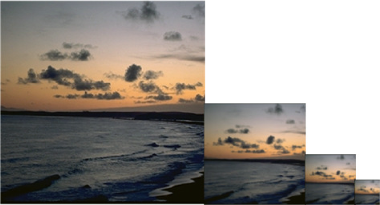
An estimate for l(x) is found by finding the MAP estimate of s(x) using the Iterated Conditional Modes (ICM) algorithm [30]. The ICM algorithm gives a sub-optimal estimate of s(x). The converged estimate represents a local optimization in the posterior formulation. Importantly, a good initialization of unknown random variables is necessary to ensure that the converged result is close to the global optimization. A multi-resolution scheme is incorporated into the algorithm. Using multi-resolution allows faster convergence for the state field s(x). The final result is more likely to converge to the global maximum. A hierarchical pyramid [31] of differing resolution is conducted (Figure 1). At the bottom level of the pyramid, the resolution was down-sampled by a factor of two in each dimension. The algorithm proceeds by initializing random variables at the coarsest level of the pyramid. An estimate of s(x) at the coarsest level (four levels are used) is obtained from the probabilistic framework, and the new estimate is then used to initializing the framework at level below. This process continues until s(x) has been estimated at full resolution. Notably, before solving l(x), the EM solving described in Equations 6 and 7 need to be finished for solving spatial likelihood in the posterior expression.
3. Experiments
To justify our proposed algorithm, we compared our method with [25] and [8]. In our implementation of [25], the Gaussian mixture model [32] and an approximated histogram of orientation of rain streaks are adopted. The character of neighboring frames of rain steaks is applied in [8]’s implementation. To evaluate the accuracy of the detection algorithm, the test video sequences contain illumination variations, camera motions, moving objects, etc. In our proposed algorithm, temporal and spatial constraints are unified into a maximum a posteriori (MAP) computation. The assumption of temporal domain is pathological motion, and the assumption of spatial domain is consistency of gradient orientation. All constraints are organized into the final estimation of unknown variables. The implemented algorithm was developed with Microsoft Visual Studio 2010 and OpenCV 2.3. The hardware configuration is composed of Intel Core(TM) i5-4200 (1.6 GHz) and 4 GB RAM. The operation system is Windows 7. Under these configurations, the average processing speed of our proposed method is about 8 images per second for 720×480 resolution sequences, whereas the methods of [25] and [8] are close to 5 images per second. That is, we get a higher processing speed due to simplified motion estimation and ICM solving. In addition to the benefit of speed, we also show the experimental results of subjective and objective assessments in following paragraph.
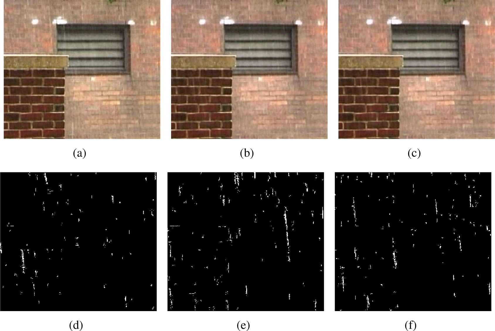
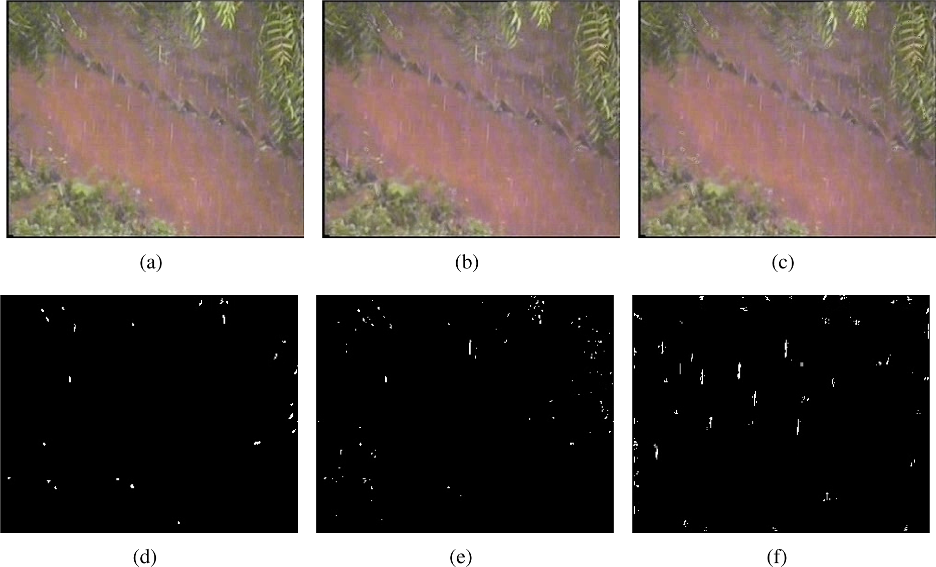
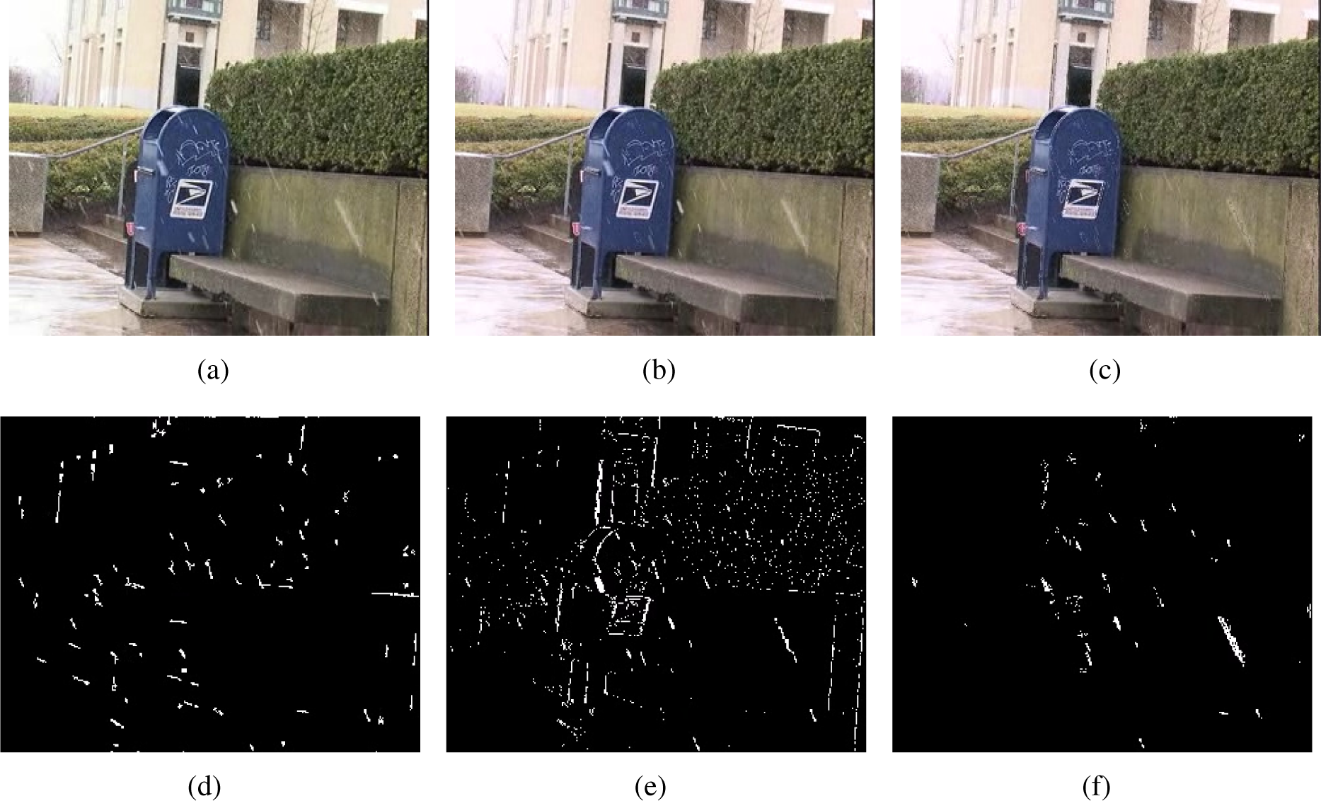
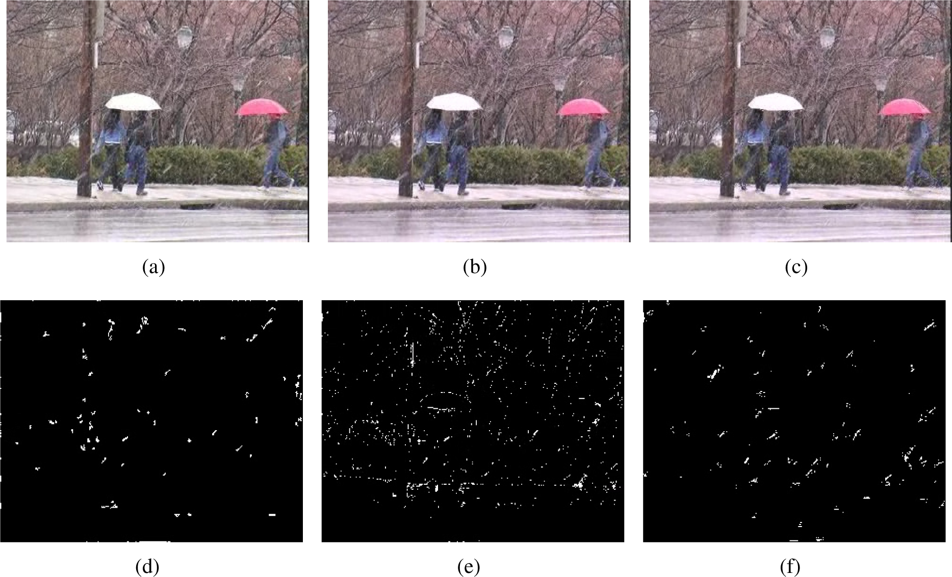
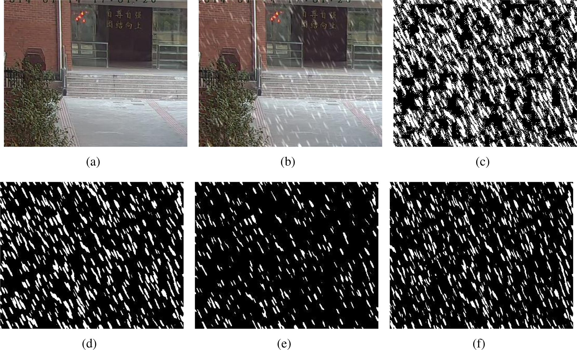
Figure 2a is the original video frame. Figure 2e is the detection mask obtained by method [25]. Figure 2b is the rain-removal frame using the detection mask of Figure 2e. Figure 2f is the detection mask obtained by method [8]. Figure 2c is the rain-removal frame using the detection mask of Figure 2f. Figure 2g is the detection mask obtained by our proposed method. Figure 2d is the rain-removal frame using the detection mask of Figure 2g. From Figure 2 to Figure 6, it can be seen that our result shows better rationality comparing with [25], [8]. Especially, the superior advantage is demonstrated in Figures 3–6. In addition to the subjective test, an objective test is also given to show the comparison of detection accuracy in Figure 7. Figure 7a is a non-rain image. Figure 7b is a synthetic image with added rain by using image editing software. Figure 7c is the ground truth of the detection mask. Figure 7d is our detection mask. Figure 7e and Figure 7f are the results of [25] and [8].
We use the numbers of detected rain pixels to feature detection accuracy which is based on the comparison between ground truth and test results. For our method, 176, 699 pixels are detected as rain, whereas 7366 and 9564 are detected using [25] and [8]. Therefore, our proposed algorithm has both higher detection accuracy and higher speed. In this objective test, false detection rate is not been considered, because rain detection is more important than non-rain detection in our image processing application. Totally, these experimental examples showcase the benefits of our algorithm. In fact, image/video spatial and temporal constraints are applied in [25] and [8], respectively. However, spatial distribution and temporal motion of rain streaks are equally important for rain detection. The methods of [25] and [8] built the framework of rain detection based respectively on spatial and temporal analysis. In contrast, we harmonize a temporal constraint and the spatial distribution of gradient of orientation into our Bayesian probabilistic framework. In order to make full use of image self-similarity and maintain image smoothness across or within the edge, as well as to strengthen the correlation of neighboring pixels, a transformed MRF is utilized in the Bayesian framework. Therefore, comparing with previous method, our method enables superior detection by combining spatial and temporal constraints, both subjectively and objectively.
4. Conclusions
In this paper, we developed a Bayesian probabilistic approach to solve the rain streaks detection problem. We differ from previous method in a number of aspects, i.e., (1) we built a Bayesian framework for detection, (2) we introduced spatial and temporal likelihood and MRF prior, (3) we used EM algorithm for parameter estimation. To sum up, our algorithm has implemented rain detection under a probabilistic framework, and compares favorably with previous method.
Acknowledgments
This work was supported by Science and Technology Innovation Foundation of Science and Technology Commission of Shanghai Municipality (12DZ0503300) and the Opening Project of Shanghai Key Laboratory of Digital Media Processing and Transmission.
Author Contributions
Chen Yao is the idea originator, who designed the algorithm and wrote the whole paper. Ci Wang made the verification of theory. Lijuan Hong and Yunfei Cheng made measurements. All authors have read and approved the final manuscript.
Conflicts of Interest
The authors declare no conflict of interest.
References
- Gilbert, A.; Giles, M.; Flachs, G.; Rogers, R.; Hsun, U. A real-time video tracking system. IEEE Trans. Pattern Anal. Mach. Intell 1980, 1, 47–56. [Google Scholar]
- Lowe, D. Object Recognition from Local Scale-invariant Features, Proceedings of the Seventh IEEE International Conference on Computer Vision, Kerkyra, Greek, 20–27 September 1999; pp. 1150–1157.
- Ke, Y.; Sukthankar, R.; Hebert, M. Efficient Visual Event Detection Using Volumetric Features, Proceedings of the Tenth IEEE International Conference on Computer Vision, Beijing, China, 17–21 October 2005; pp. 166–173.
- Itti, L.; Koch, C.; Niebur, E. A model of saliency-based visual attention for rapid scene analysis. IEEE Trans. Pattern Anal. Mach. Intell 1998, 20, 1254–1259. [Google Scholar]
- Lucas, B.; Kanade, T. An iterative image registration technique with an application to stereo vision, Proceedings of the 7th International Joint Conference on Artificial Intelligence, Milan, Italy, 24–28 August 1981.
- Portabella, M.; Stoffelen, A. Rain detection and quality control of SeaWinds. J. Atmos. Ocean. Tech 2001, 18, 1171–1183. [Google Scholar]
- Chen, R.; Chang, F.; Li, Z.; Ferraro, R.; Weng, F. Impact of the vertical variation of cloud droplet size on the estimation of cloud liquid water path and rain detection. J. Atmos. Sci 2007, 64, 3843–3853. [Google Scholar]
- Garg, K.; Nayar, S. Detection and removal of rain from videos, Proceedings of the 2004 IEEE Computer Society Conference on Computer Vision and Pattern Recognition, Washington, DC, USA, 27 June–2 July 2004.
- Garg, K.; Nayar, S. Vision and rain. Int. J. Comput. Vision 2007, 75, 3–27. [Google Scholar]
- Garg, K.; Nayar, S. Photorealistic rendering of rain streaks. In ACM Transactions on Graphics (TOG); ACM: New York, NY, USA, 2006; Volume 25, pp. 996–1002. [Google Scholar]
- Hase, H.; Miyake, K.; Yoneda, M. Real-time snowfall noise elimination, Proceedings of the 1999 International Conference on Image Processing, Kobe, Japan, 24–28 October 1999; 2, pp. 406–409.
- Zhang, X.; Li, H.; Qi, Y.; Leow, W.; Ng, T. Rain removal in video by combining temporal and chromatic properties, Proceedings of the 2006 IEEE International Conference on Multimedia and Expo, Ontario, Canada, 9–12 July 2006; pp. 461–464.
- Brewer, N.; Liu, N. Using the shape characteristics of rain to identify and remove rain from video. Struct. Syntactic Stat. Pattern Recognit 2008, 5342, 451–458. [Google Scholar]
- Barnum, P.; Narasimhan, S.; Kanade, T. Analysis of rain and snow in frequency space. Int. J. Comput. Vision 2010, 86, 256–274. [Google Scholar]
- Barnum, P.; Kanade, T.; Narasimhan, S. Spatio-temporal frequency analysis for removing rain and snow from videos, Proceedings of the Workshop on Photometric Analysis For Computer Vision (PACV), Rio de Janeiro, Brazil, 14–21 October 2007.
- Kang, L.; Lin, C.; Fu, Y. Automatic single-image-based rain streaks removal via image decomposition. IEEE Trans. Image Process 2011. [Google Scholar] [CrossRef]
- Starck, J.; Moudden, Y.; Bobin, J.; Elad, M.; Donoho, D. Morphological component analysis, Proceedings of the SPIE Conference Wavelets. Citeseer, San Diego, CA, USA, 31 July–4 August 2005.
- Fadili, J.; Starck, J.; Elad, M.; Donoho, D. Mcalab: Reproducible research in signal and image decomposition and inpainting. Comput. Sci. Eng 2010, 12, 44–63. [Google Scholar]
- Buades, A.; Coll, B.; Morel, J. A review of image denoising algorithms, with a new one. SIAM J. Multiscale Model. Simul 2005, 4, 490–530. [Google Scholar]
- Elad, M.; Aharon, M. Image denoising via sparse and redundant representations over learned dictionaries. IEEE Trans. Image Process 2006, 15, 3736–3745. [Google Scholar]
- Aharon, M.; Elad, M.; Bruckstein, A. -SVD: An Algorithm for Designing Overcomplete Dictionaries for Sparse Representation. IEEE Trans. Signal Process 2006, 54, 4311–4322. [Google Scholar]
- Mairal, J.; Elad, M.; Sapiro, G. Sparse representation for color image restoration. IEEE Trans. Image Process 2008, 17, 53–69. [Google Scholar]
- Tomasi, C.; Manduchi, R. Bilateral filtering for gray and color images, Proceedings of the Sixth International Conference on IEEE Computer Vision, Bombay, India, 4–7 January 1998; pp. 839–846.
- Zhang, M.; Gunturk, B. Multiresolution bilateral filtering for image denoising. IEEE Trans. Image Process 2008, 17, 2324–2333. [Google Scholar]
- Bossu, J.; Hautière, N.; Tarel, J. Rain or snow detection in image sequences through use of a histogram of orientation of streaks. Int. J. Comput. Vision 2011, 93, 348–367. [Google Scholar]
- Dean, N.; Raftery, A. Normal uniform mixture differential gene expression detection for cDNA microarrays. BMC Bioinform 2005, 6, 173. [Google Scholar]
- Kokaram, A. On missing data treatment for degraded video and film archives: A survey and a new bayesian approach. IEEE Trans. Image Process 2004, 13, 397–415. [Google Scholar]
- Corrigan, D.; Harte, N.; Kokaram, A. Pathological motion detection for robust missing data treatment. EURASIP J. Adv. Signal Process 2008, 2008, 153. [Google Scholar]
- Noda, H.; Shirazi, M.; Kawaguchi, E. MRF-based texture segmentation using wavelet decomposed images. Pattern Recog 2002, 35, 771–782. [Google Scholar]
- Greig, D.; Porteous, B.; Seheult, A. Exact maximum a posteriori estimation for binary images. J. R. Stat. Soc. Ser. B 1989, 51, 271–279. [Google Scholar]
- Bergen, J.; Anandan, P.; Hanna, K.; Hingorani, R. Hierarchical model-based motion estimation. In Computer Vision—ECCV’92; Springer: Berlin/Heidelberg, Germany, 1992; pp. 237–252. [Google Scholar]
- Zivkovic, Z. Improved adaptive Gaussian mixture model for background subtraction, Proceedings of the IEEE 17th International Conference on Pattern Recognition, 2004, Cambridge, UK, 23–26 August 2004; 2, pp. 28–31.


| s(x) | t(x) | l(x) | s(x) | t(x) | l(x) |
|---|---|---|---|---|---|
| 0 | 0, 0, 0, 0 | 0 | 8 | 1, 0, 0, 0 | 0 |
| 1 | 0, 0, 0, 1 | 0 | 9 | 1, 0, 0, 1 | 0 |
| 2 | 0, 0, 1, 0 | 0 | 10 | 1, 0, 1, 0 | 0 |
| 3 | 0, 0, 1, 1 | 1 | 11 | 1, 0, 1, 1 | 1 |
| 4 | 0, 1, 0, 0 | 0 | 12 | 1, 1, 0, 0 | 1 |
| 5 | 0, 1, 0, 1 | 0 | 13 | 1, 1, 0, 1 | 1 |
| 6 | 0, 1, 1, 0 | 1 | 14 | 1, 1, 1, 0 | 1 |
| 7 | 0, 1, 1, 1 | 1 | 15 | 1, 1, 1, 1 | 1 |
© 2014 by the authors; licensee MDPI, Basel, Switzerland This article is an open access article distributed under the terms and conditions of the Creative Commons Attribution license (http://creativecommons.org/licenses/by/3.0/).
Share and Cite
Yao, C.; Wang, C.; Hong, L.; Cheng, Y. A Bayesian Probabilistic Framework for Rain Detection. Entropy 2014, 16, 3302-3314. https://doi.org/10.3390/e16063302
Yao C, Wang C, Hong L, Cheng Y. A Bayesian Probabilistic Framework for Rain Detection. Entropy. 2014; 16(6):3302-3314. https://doi.org/10.3390/e16063302
Chicago/Turabian StyleYao, Chen, Ci Wang, Lijuan Hong, and Yunfei Cheng. 2014. "A Bayesian Probabilistic Framework for Rain Detection" Entropy 16, no. 6: 3302-3314. https://doi.org/10.3390/e16063302