Searching for Conservation Laws in Brain Dynamics—BOLD Flux and Source Imaging

Abstract

Blood-oxygen-level-dependent (BOLD) imaging is the most important noninvasive tool to map human brain function. It relies on local blood-flow changes controlled by neurovascular coupling effects, usually in response to some cognitive or perceptual task. In this contribution we ask if the spatiotemporal dynamics of the BOLD signal can be modeled by a conservation law. In analogy to the description of physical laws, which often can be derived from some underlying conservation law, identification of conservation laws in the brain could lead to new models for the functional organization of the brain. Our model is independent of the nature of the conservation law, but we discuss possible hints and motivations for conservation laws. For example, globally limited blood supply and local competition between brain regions for blood might restrict the large scale BOLD signal in certain ways that could be observable. One proposed selective pressure for the evolution of such conservation laws is the closed volume of the skull limiting the expansion of brain tissue by increases in blood volume. These ideas are demonstrated on a mental motor imagery fMRI experiment, in which functional brain activation was mapped in a group of volunteers imagining themselves swimming. In order to search for local conservation laws during this complex cognitive process, we derived maps of quantities resulting from spatial interaction of the BOLD amplitudes. Specifically, we mapped fluxes and sources of the BOLD signal, terms that would appear in a description by a continuity equation. Whereas we cannot present final answers with the particular analysis of this particular experiment, some results seem to be non-trivial. For example, we found that during task the group BOLD flux covered more widespread regions than identified by conventional BOLD mapping and was always increasing during task. It is our hope that these results motivate more work towards the search for conservation laws in neuroimaging experiments or at least towards imaging procedures based on spatial interactions of signals. The payoff could be new models for the dynamics of the healthy brain or more sensitive clinical imaging approaches, respectively.

1. Introduction

Understanding functional mechanisms underlying brain dynamics is essential for clinical applications such as recovery from stroke, traumatic brain injury, and disorders of consciousness. Neuronal activity in response to perceptual stimuli or cognitive tasks can be mapped by using the blood-oxygen-level-dependent (BOLD) response as a proxy signal in functional MRI experiments. Functional MRI (fMRI) studies have provided us with detailed insights into local functional organization of the brain. Recently, fMRI also has allowed for mapping of brain networks, mostly during unconstrained tasks or “rest”. Whereas physiological models exist that describe the local relationship of neuronal processing, hemodynamics, and the observed signal [1–3], which can be numerically validated [4,5], the physiology underlying the spatial relationships among signals is much less understood [6–9]. Nevertheless, many recent studies relate BOLD resting state networks to functional networks of the brain, for example by utilizing information theoretical concepts or other notions from physics such as small world networks [10–14].

Despite these efforts to link BOLD signals of the brain to physical concepts, it seems that one fundamental way of physical modeling has not been applied to functional brain imaging yet: The concept of conserved quantities and conservation laws. Most laws of modern physics can be derived from conservation laws, which again follow from fundamental properties of the world such as space and time homogeneity. As the brain becomes more and more understood as a neurovascular system, and as functional imaging technologies can depict brain function with reasonable high spatial resolution, in this contribution we ask: Does the brain described on spatiotemporal scales accessible with fMRI experiments reveal conservation laws of observable quantities that might assist us in modeling brain dynamics? Although we will not be able to provide final answers within this manuscript, we hope that the proposed research methodology will inspire more applications in the quest for a better understanding of spatiotemporal brain dynamics.

As a first step towards this goal, we performed an fMRI experiment on a group of nine healthy subjects, in which the response to a complex mental motor imagery task [15] was mapped. We then quantified the spatial relationship between local BOLD signals in order to define BOLD fluxes, sources and sinks. Conservation laws then might show up as a balance between sources and sinks, for example.

The manuscript is organized as follows: We briefly review the importance of conservation laws and mention possible hints for conservation laws affecting brain dynamics (Section 2). We then describe a model based on continuity equations and associated quantities such as fluxes and sources (Section 3). These quantities are then measured in an fMRI imaging experiment (Section 4). Although this experiment does not provide definite answers yet, it provides hints for a more global organization of brain function not seen before in conventional BOLD mapping (Section 5). A discussion concludes the paper (Sections 6).

2. Do Conservation Laws Rule the Brain?

2.1. The Importance of Conservation Laws

We are aiming at a description of the spatiotemporal dynamics of the BOLD signal by physical principles. The reason is that physical models of complex systems are often generalized models encompassing a whole class of specific systems. For example, many different pattern-forming systems can be described by generalized equations independent of the specifics of the system’s components [16]. Similarly, conserved quantities such as energy, mass, or momentum are applicable for a wide range of systems. In this sense, we are not aiming at describing the spatiotemporal dynamics of the brain by specific physiological parameters (although this is of course a desirable goal, too), but on a phenomenological level by general physical laws.

In particular, conservation laws state that certain system properties do not change as the system evolves, or, if they change, how they are balanced by sources and sinks. For example, the total energy is conserved for many systems during time evolution, but not necessarily the entropy [17,18]. In particular for systems out of equilibrium there are models for the entropy that take its change into account by assigning it to source terms [19].

Here we are interested in conservation laws, including non-conserved quantities described by sources and sinks, for two reasons: (i) There exists a quite general way of expressing conservation laws in spatiotemporal systems without the need to specify the specific nature of the quantity: Continuity equations explicitly relate the local change of a physical quantity to nonlocal influences, namely flow or flux terms, and to source and sink terms. (ii) On a certain level of description, the brain can be considered as a flow-equilibrium system, which naturally gives rise to a possible description by continuity equations.

2.2. Possible Hints for Conservation Laws Ruling the Brain

It is well known that the brain consumes, relative to its contribution to body mass, an over-proportional amount of energy [20]. During normal brain operation, blood continuously transports the main source of energy, glucose and oxygen, into the brain, and waste is exported in the same way. On average, the inflow of blood into the brain must equal the outflow. This already gives rise to a mass conservation law that can principally be expressed by continuity equations. Similar mass conservation laws will hold for smaller vessels down to the capillary level [21,22]. In addition, cerebral autoregulation ensures that average energy supply is kept approximately in equilibrium. Unlike a muscle that consumes less energy during rest than during work, the brain seems to consume a considerable amount of energy even in its “resting” condition. Fluctuations from this background activity, which can be picked up with fMRI, for example, are thought of consuming only a small percentage of this energy [23]. Therefore, seen as a physical system, even the working brain can then be considered on average to be in a flow-equilibrium. In addition, tight energy constraints on the brain created a highly optimized organ with probably little energy to waste [24]. It stands to reason that flow-equilibrium together with optimized energy usage might give rise to conserved quantities even trickling down to local levels of description.

The simplest sign of conserved quantities observable in BOLD signals would be a negative response that on average offsets the positive responses. However, in many experimental tasks including the one used in this paper, negative responses are not seen consistently and therefore do not persist on a group level analysis over subjects. Local negative responses do exist however and have been consistently found in occipital cortex in humans [25], adjacent to regions with positive response. Negative responses have been related to decreased neuronal activation [26–28] but also alternatives such as reallocation of resources and hemodynamic effects [29–31] have been proposed. Further, negative responses have been observed in high-resolution imaging of cortical layers [32], in pathological conditions [33–35], to noxious stimuli [36], and, again adjacent to positive responses, in indirect response to optogenetic stimulation [5,37,38]. Notwithstanding the still debated origins of negative BOLD [39,40], these and other observations of negative BOLD show that there might be mechanisms of neuronal, vascular, or neurovascular organization that could involve yet to be determined conserved quantities.

There is another hint towards an organization of global brain dynamics that might give rise to conservation laws: During rest, BOLD amplitude baseline fluctuations exhibit a well-defined spatiotemporal dynamics [6,7]. The most prominent resting state network, the “default mode” was originally discovered in resting PET data [41] but also reveals itself in resting state as well as task-dependent BOLD [8,9]. There are task-positive as well as task-negative responses of areas belonging to the default mode network during attention demanding tasks or goal directed behavior [41,42]. A biological selective pressure for the evolution of conservation laws controlling the distribution and regulation of changes in blood flow in the brain is the closed volume of the skull somewhat limiting the expansion of brain tissue by increases in blood volume [43]. An active law-like reallocation of blood volume based on the regularities of correlations of components of the specific neuronal networks identified in studies of the resting state [44–46] may help keep intracranial blood volume relatively constant over the wide range of blood pressures seen in the flat part of the cerebral autoregulation curve.

As another argument for the possible importance of conservation laws in brain dynamics we cite very recent work that found conservation laws ruling at completely different time scales: biological brain evolution, brain growth, and ageing, demonstrated on cortical minicolumns [47]. These findings concern structural changes of the brain, but brain growth and ageing also can be seen as very slow dynamical changes.

Finally, from cognitive-behavioral studies it becomes more and more appreciated that attention is directed at only one (or at most two [48]) goals at a time and that “multitasking” [49] of the brain probably is really a shift of attention between multiple cognitively demanding tasks. This phenomenon shows that some parts of the brain, even if thought to be attributed to different tasks, probably cannot function independently at the same time. One might be tempted to speculate that the phenomenon of attention focusing follows from constraints on the total computational power of the neuronal network of the brain, or in other words, a conservation law.

3. Theory

3.1. Continuity Equations

We are aiming at an interpretation of data in terms of continuity equations, which are tightly connected to the concept of conserved quantities. The continuity equations used in fluid dynamics, electromagnetism, and many other physical disciplines relate the time change of a quantity to fluxes and sources of that quantity. Continuity equations are either differential or integral equations, which are related to each other by the Gauss theorem. Here we use the differential notation because differential quantitates better suit the local estimation approach that we are adopting for the analysis of fMRI data. However, integral equations might be advantageous for further analysis procedures not described here, for example to measure the fluxes into or out of particular brain regions.

Our main assumption is that the BOLD amplitude represents a density or concentration of something that can drive a gradient flux, and that we can neglect advective flux on this level of description. If the observed BOLD amplitude in an imaging voxel located at position r = (x, y, z) and time t is denoted by ρ(r,t), the corresponding gradient flux j(r,t) = (j_x(r,t), j_y(r,t), j_z(r,t)) can be written as:

$$\mathbf{j}(\mathbf{r},\text{t})=-\text{D}\hspace{0.17em}\text{grad}\hspace{0.17em}\rho (\mathbf{r},\text{t})$$

(1)

The constant D relates the magnitude of the flux to the concentration gradient grad ρ(r,t) = (∂ρ(r,t)/∂x, ∂ρ(r,t)/∂y, ∂ρ(r,t)/∂z)), and is assumed constant in space and time. In the neurovascular coupling balloon model of Buxton and others [2,3,50–52], the BOLD signal is a nonlinear function of blood deoxyhemoglobin content and blood volume. As a working hypothesis we therefore assume that blood volume or hemoglobin concentrations can influence neighboring regions in the way as described by Equation (1), either directly or mediated by neuronal activity. Without specifying the underlying physiological mechanisms, here we just use our working hypothesis in order to test for a continuity equation of the BOLD signal that might have to be modified in further searches for conservation laws. The continuity equation:

$$\partial \rho (\mathbf{r},\text{t})/\partial \text{t}+\text{div}\hspace{0.17em}\mathbf{j}(\mathbf{r},\text{t})=\sigma (\mathbf{r},\text{t})$$

(2)

where div j(r,t) = ∂j_x(r,t)/∂x + ∂j_y(r,t)/∂y + ∂j_z(r,t)/∂z is the divergence of the flux j(r,t) and σ(r,t) a source term, can now be written as:

$$\partial \rho (\mathbf{r},\text{t})/\partial \text{t}=\text{D}\hspace{0.17em}\Delta \hspace{0.17em}\rho (\mathbf{r},\text{t})+\sigma (\mathbf{r},\text{t})$$

(3)

with the Laplace operator Δ = div grad = ∂²/∂x² + ∂²/∂y² + ∂²/∂z².

In an fMRI block design experiment, one typically has two alternating states, periods of task execution followed by control periods of rest. Denoting the task state with “1” and the control state with “0”, from Equation (3) follows:

$$\partial {\rho }_0(\mathbf{r},\text{t})/\partial \text{t}=\text{D}\hspace{0.17em}\Delta \hspace{0.17em}{\rho }_0(\mathbf{r},\text{t})+{\sigma }_0(\mathbf{r},\text{t})\hspace{0.17em}\text{and}\hspace{0.17em}\hspace{0.17em}\partial {\rho }_1(\mathbf{r},\text{t})/\partial \text{t}=\text{D}\hspace{0.17em}\Delta \hspace{0.17em}{\rho }_1(\mathbf{r},\text{t})+{\sigma }_1(\mathbf{r},\text{t})$$

(4)

Finally, the BOLD response is approximated as a block function proportional to a characteristic function consisting of “0”s and “1”s indicating periods of rest and task, respectively: During rest, ρ₀(r,t) = ρ₀(r), during task, ρ₁(r,t) = ρ₁(r). In other words, the BOLD amplitude is modeled as constant over time (but not space) during task and control periods and its explicit time derivatives vanish. Therefore, we end up with expressions for the BOLD sources tailored to a simple block design fMRI experiment:

$${\sigma }_0(\mathbf{r})=-\text{D}\hspace{0.17em}\Delta \hspace{0.17em}{\rho }_0(\mathbf{r})\hspace{0.17em}\hspace{0.17em}\text{and}\hspace{0.17em}\hspace{0.17em}{\sigma }_1(\mathbf{r})=-\text{D}\hspace{0.17em}\hspace{0.17em}\Delta \hspace{0.17em}\hspace{0.17em}{\rho }_1(\mathbf{r})$$

(5)

In other words, the Laplacians of the BOLD signal for task and control blocks provide estimates for the sources, up to a constant. It is this variable then that is regressed against the characteristic function in order to estimate an effect, instead of the BOLD amplitude itself.

3.2. Estimation of Fluxes and Sources from BOLD Data

To estimate sources of the BOLD signal, as per Equation (5) the Laplacians of the signals need to be computed for each voxel and time point. The Laplacian can be approximated by a finite difference scheme that involves nearest neighbor voxels. Here we adopt a scheme that is accurate to second order in the time interval [53] in order to avoid having to use voxels further away from the voxel of interest, which could blur the estimate. Estimation of the fluxes j(r,t), up to the constant D, works equivalently by computing the numerical gradient for second order accuracy (Equation (1)). However, the three components of j(r,t) each on their own do not contain much information. Therefore, in the application we test for the hypothesis that the Euclidean norms of j₀(r,t) and j₁(r,t) do not differ. This hypothesis does not account for changes of direction, unfortunately, and there is still room for improvement. The details of the statistical procedures as applied to experimental data are provided in Section 4.

3.3. Generalizations

If the explicit time dependence of the BOLD amplitude ρ(r,t) has to be taken into account, for example in the case of slow changes that cannot be described by a block function, or when there are no defined alternating task and rest periods such as in resting state fMRI, Equation (5) does not hold. In this case, ∂ρ(r,t)/∂t needs to be estimated from data, too, and used as an additional regressor. For example, in a two-variable regression model with the variables ∂ρ(r,t)/∂t and Δ ρ(r,t), where D is then the fit coefficient (see Equation (3)), the sources σ(r,t) would have to be defined differently. It depends on the specific situation if these are valid assumption and is not topic of this paper.

4. Mapping BOLD Fluxes and Sources in a Motor Imagery Experiment

4.1. Motivation

In mental motor imagery or short motor imagery [15,54] subjects are imagining themselves performing a motor activity. Here we chose this kind of task as it normally elicits strong BOLD responses in various brain areas [55–64], and due to its widespread application in the study of disorders of consciousness [65,66].

4.2. Subjects

Experiments were performed on nine healthy adult subjects (37 ± 8 years, one female) and one 23-year-old man who had had a severe traumatic brain injury about 4 years before scanning. All experiments were approved by the Institutional Review Board of Weill Cornell Medical College, and informed consent was obtained from the subjects or their proxies.

4.3. MRI

Data were acquired on a 3.0 T General Electric MRI scanner (healthy subjects) and on a 3.0 T Siemens TIM Trio MRI scanner (patient). For fMRI, a GE-EPI sequence was used (TR = 2 s, TE = 30 ms, flip angle = 70°, voxel size = 3.75 × 3.75 × 5 mm on the GE and 3.75 × 3.75 × 4 mm on the Siemens scanner). Before the scan, the healthy subjects were instructed to imagine themselves swimming, starting and stopping with pre-recorded cues received over MRI compatible headphones. The patient was instructed to imagine himself swinging a tennis racket with his right hand, and cues were delivered over in-room loudspeakers. In the interim, all subjects were required to think of nothing in particular. Eight blocks of 16 s rest alternating with 16 s task were used. Data acquisition consisted of 128 scans with a total time of 4:16 min. In addition, anatomical high-resolution scans of the whole head were acquired.

4.4. fMRI Data Analysis

The following preprocessing procedures were applied using SPM5 [10]: motion correction, slice timing correction, and spatial normalization to an MNI template [icbm_avg_152_t1_tal_lin.mnc, MNI, Canada (ICBM, NIH P-20 project)], including interpolation to a voxel size of 2 × 2 × 2 mm. Then, using Matlab, the data was normalized by subtracting the mean over all voxels and time points and then dividing by the standard deviation over all voxels and time points. Note that we did not normalize each voxel time series by its own mean and standard deviation as this would render the spatial derivatives, computed later on, useless after averaging. Each voxel time series was then high-pass filtered with a cutoff frequency of 0.01 Hz. A characteristic function consisting of “0”s and “1”s indicating blocks of eight samples was shifted two samples against the functional paradigm to account for hemodynamic delay. We did not use a more detailed hemodynamic model in order to keep the analysis comparable between conventional BOLD amplitude mapping and our approach of spatial interaction of amplitudes mapping.

(1)

Conventional BOLD amplitude mapping: The linear correlation coefficient between the characteristic function and each preprocessed voxel time series was converted into z-values by Fisher’s z-transform [67]. This linear least-squares procedure models the case that the relationship between data and characteristic function is linear with unexplained variance expressed through normally distributed residuals.

(2)

Spatial interaction of BOLD amplitude mapping: For each voxel, the linear correlation coefficient between the characteristic function and the flux norm was computed and converted to z-values. A positive z-value means that during the task the absolute value of the flux as per Equation (1) increases. The procedure was repeated for the source estimate as per Equation (5). Again, any unexplained variance is modeled by normally distributed residuals.

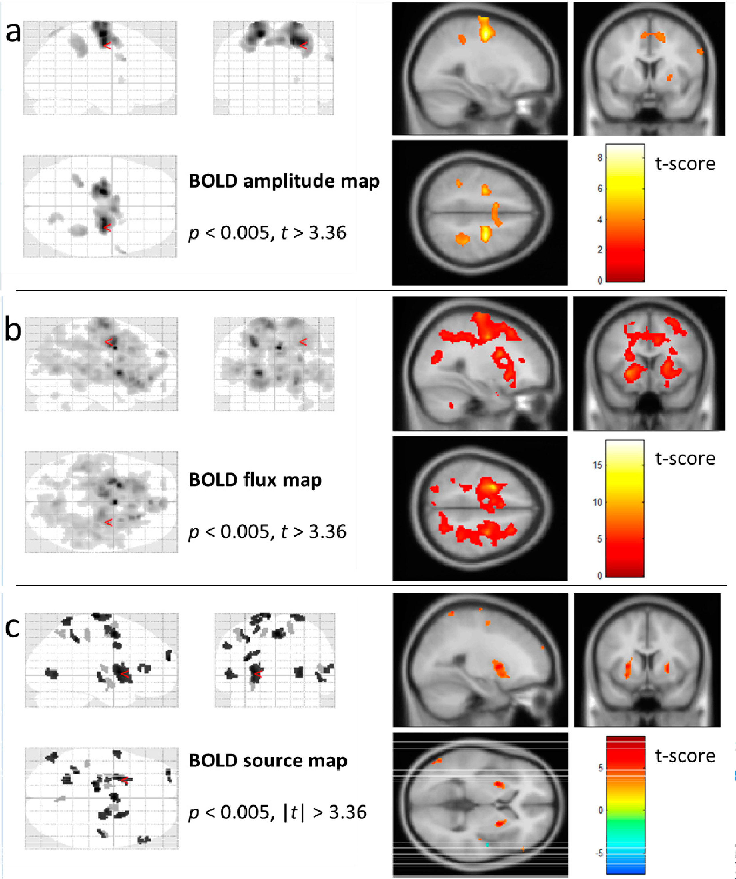
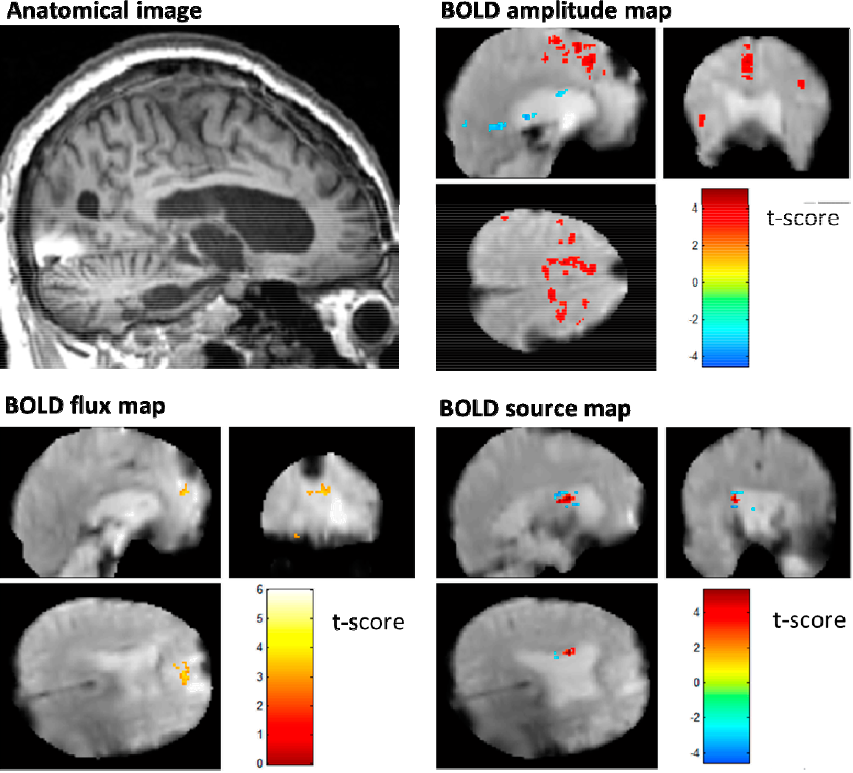
For the group analysis, the z-maps were spatially smoothed with SPM5 with an 8 mm full-width-half-mean Gaussian kernel [68]. Subsequently, a mixed effects group analysis of all nine scans was performed on those z-maps, in which the z-values were used as the fit coefficients. This quite conservative approach includes inter-subject variance and allows for inference on the population level. The null hypothesis tested was that this group does not activate on average, using a one-sample t-test within a summary statistics approach, as typical in a mixed (or random) effects analysis in SPM [69]. The occurrence of false positives in the group SPMs of the flux was controlled by using a false-discovery rate (FDR) of q = 0.04, based on the data masked by the MNI template to exclude most extracerebral voxels, and computed by xjView ( http://www.alivelearn.net/xjview); in the flux map, q = 0.04 corresponds to an uncorrected p < 0.005, which was used in all other maps. Also, clusters smaller than 27 voxels were discarded. Fixing the threshold to p < 0.005 (t > 3.36) was necessary for two reasons: (1). to make different maps comparable as the FDR critically depends on the volume of activation. (2). It was not possible for example to fix q = 0.05 as otherwise the clear and strong BOLD amplitude map observed, concordant with literature results in motor imagery [15,54–57,59,61,63], would not have shown up in this conservative analysis, although visible in all individual subjects. Maximal intensity projections or “glass brains” and SPMs were finally displayed by xjView, too.

For the case study subject in the discussion section, no smoothing was applied and the threshold for p < 0.005 was set to |t| > 2.81 under the assumption of a z-distribution due to the larger number of degrees of freedom now available.

5. Results

5.1. BOLD Amplitude Mapping

A conventional BOLD amplitude group map revealed positive activation bilaterally in one cluster covering mostly premotor and supplementary motor areas in BA6 (p < 0.005, t = 3.36). A glass brain and t-map are shown in Figure 1(a). Additionally, there was significant positive bilateral BOLD response in the superior and inferior parietal gyri, and a small cluster within the right putamen. No negative BOLD response was observed.

5.2. BOLD Flux Mapping

The first map based on a spatial analysis of the BOLD signal, the BOLD flux map (Figure 1(b)), revealed more widespread positive values with considerable overlap to premotor cortex and smaller overlap to areas located towards the interhemispheric fissure (SMA). In addition, there was congruency with superior and inferior parietal gyri. Notable additional increased flux during task was observed in the mid and anterior cingulate gyrus, the calcarine sulcus, cuneus and precuneus, and bilaterally in the superior temporal gyrus. In addition, there were larger clusters, now bilateral, in the putamen. Again, no negative response was observed.

5.3. BOLD Source Mapping

The second map based on a spatial analysis of the BOLD signal, the BOLD source map (Figure 1(c)), revealed both positive and negative values (see also Figure 2(a), right panel). The largest positive cluster (i.e., BOLD source) was located bilaterally in the putamen, and the second largest cluster in the SMA. Comparatively small clusters included locations in the left precentral gyrus, the right and left superior frontal gyrus, and the left superior and inferior parietal gyrus. Negative values (i.e., BOLD sink) were observed in small parts of the SMA but were located more towards adjacent white matter regions (Figure 2(a), right). Additional very small regions of negative values included the left postcentral gyrus, the precuneus, right Heschl’s gyrus, and left amygdala. These small regions might be more likely to be false positives as we did not strictly correct for multiple comparison specific to source mapping but used the same p-values as for BOLD flux mapping, or leakage from the auditory stimuli.

6. Discussion

6.1. Implications towards Conservation Laws Affecting Neuronal Dynamics

To summarize the findings: The conventional BOLD amplitude map is in agreement with previously published fMRI motor imagery experiments [15,54–60,62,64,70]. BOLD flux maps were more widespread than BOLD amplitude maps, but there were also regions in BOLD amplitude responses without corresponding increases in BOLD flux in the SMA. BOLD sources were mostly restricted to the putamen and SMA, whereas BOLD sinks were only sparsely distributed and small.

Taken together, it is not too evident that the sources and sinks can account for all the increased fluxes during task observed for example in the cingulate cortex. On the other hand, there were promising hints towards a continuity equation: Detectable sources in the SMA surrounded by flux, and also sources in the putamen. Overall, the observations do not seem to point strongly towards or against our main hypothesis of conserved quantities governed by a continuity equation.

There could be a number of reasons, including: First, it might be an interpretation difficulty as there is no experience with how the flux, source and sink patterns actually should appear in the brain. Second, the sought processes might be sub-threshold and not showing in this quite conservative statistical approach used. Also, the use of derivatives increases noise and might mask the sought effects. By using derivatives, we are actually doing the opposite of the conventional smoothing approach of fMRI data analysis, where smoothing is used in order to reduce the noise by averaging [10,71,72]. Third, model inadequacy; it might be that some model assumptions, such as the homogeneity of the constant D, are not valid approximations, for example due to inhomogeneities in vascularity, neuronal density, etc.. Also, the model neglects energy storage within the brain, for example in the form of ionic gradients and releasable transmitter, such that models based on instantaneous differential balances of sources and sinks are too limited to fully embrace the local energy balance [73–75]. In other words, homogeneous time-invariant model approach might be too simplistic. Fourth, the BOLD amplitude might not be the right proxy variable to use in such an analysis, or the BOLD amplitude as a nonlinear combination of other factors might mask the relevance of these factors. Therefore, other parameters such as cerebral blood flow, volume, or metabolic rate of oxygen might be more suitable. Fifth, even if there are conserved quantities, the description by a continuity equation might not be right or optimal. Finally, it might be that conservation laws just play not a major role in the dynamics of the brain on this spatiotemporal scale.

6.2. BOLD Flux Imaging and Model-Free Approaches

Our finding that the flux appears to extend well beyond areas of primary relationship to the task in a group analysis is reminiscent of recent findings that if sufficient data is measured and analyzed in a model-free way, most of the brain appears to be involved even in simple tasks [76]. Similar to that finding, our model is quite versatile as it depends on spatial correlations among voxels only, thereby dismissing information of the BOLD amplitudes themselves. More work is needed to relate BOLD flux imaging to those approaches. In addition, flux maps were derived under the assumption that flux values are distributed normally; however, due to their computation as vector norms flux distributions are skewed and it has not been investigated here if statistical tests that account for this will yield different results than the tests used here to compute flux maps.

6.3. Putamen

We found a strong BOLD source signal in particular in the putamen, meaning that during task signal fluctuations in putaminal areas become more homogeneous. This has been demonstrated recently in a similar experiment using local spatial synchronization fMRI (lssfMRI), where it was shown that during the task voxels appear more synchronized than during the control period [62]. There, it has been argued that lssfMRI might be sensitive to spatial neuronal synchronization, specifically on spatial scales accessible to BOLD fMRI. A recent investigation of such spatial synchronization measured with electrodes in the striatum of macaques [77] might support this notion: These authors found a functional specialization of the putamen in the sense that pairs of putaminal medium spiny neurons were synchronized (by means of correlation) during a classical conditioning task. In contrast, neurons in the caudate and ventral striatum were not. Specifically, the electrodes covered a region with a spatial extension accessible to fMRI.

6.4. Relation to Resting State fMRI

The here presented approach of BOLD flux and source mapping specifically probes for spatial dependencies (computed as spatial derivatives) between nearest neighbor voxels, disregarding the BOLD amplitude itself. It therefore differs somewhat from correlation-based or independent component resting state analyses [6,7,9,78,79] in which correlations between BOLD amplitudes are measured. In addition, this approach is task dependent and looks at the differences between task and control states [80]. A positive flux response here means that the norm of the BOLD gradient increases during task. A positive BOLD source signal means that the second spatial derivative decreases, indicating an increased homogeneity during the task period.

6.5. Differential Operators, Smoothing, and Nonlinear Transformations

The Laplacian is widely used in image analysis for blob detection. Blobs are areas of local homogeneity in pixel values. The here proposed source/sink estimation is based on applications of the Laplacian, too, before correlating the resulting time series voxelwise with the characteristic function of the task. From image analysis research it is known that the particular definition of the Laplacian actually pre-determines the local sensitivity, or the blob size to be detected, and it has been suggested to apply multi-scale approaches [81] to get a better picture of the blob distribution. In our application, the Laplacian has been defined by involving only nearest neighbors of the voxel of interest, thereby setting the scale or bandwidth accordingly. This can be generalized by using other spatial derivative estimators [82]. This way, the results presented here might change and more work is in order to define the optimal definition of Laplace and gradient operators.

If applied to pre-smoothed data, derivatives partially revert smoothing, if the bandwidths of the differential operators and the smoothing operator are of comparable value. Then, the source maps as defined here would not necessarily provide much new information. Therefore, it is essential that no smoothing of the data is performed beforehand.

Another issue not addressed so far is how the nonlinear transformation to MNI space and the involved interpolation to an isotropic voxel size distort the derivative estimates. For example, it might be worthwhile to compute sources and fluxes before rather than after those transformations, and then transform the resulting maps to MNI space for the subsequent group analysis.

Finally, the local anatomy of the brain given by folded cortical layers etc. might dictate better local spaces to work with than the Cartesian grid approach used by us.

6.6. Possible Clinical Applications

Once conservation laws are established for normal, healthy brain dynamics, the hope is that they would inform our understanding of altered brain function. In pathological conditions one might then use conservation laws derived from imaging to detect how the brain copes with these conditions, which might then again enable imaging modalities with better discriminatory power to diagnose disease. Whereas this is a distant goal, already we found in our group study with healthy subjects that BOLD flux imaging was comprising larger areas than conventional BOLD amplitude maps, as well as larger significance measured by t-values (Figures 1(a,b)).

In order to provide an example of an individual clinical subject analysis, rather than a group study, here we consider a subject in the minimally conscious state (MCS). The MCS is a recovery step often following the vegetative state after severe brain injuries [83]. Functional MRI in MCS can be used to locate residual cognitive capacities, for example by having subjects follow simple commands via mental motor imagery, providing data sets as used here [55,84]. These experiments can assist diagnostics in order to distinguish MCS from other conditions [85] such as the locked-in syndrome [86], in which subjects are conscious but the ability to communicate is severely limited to absent. They also might assist clinical applications such as neural control engineering or planning for brain computer interfaces [87–91]. In our previous MCS neuroimaging studies, we found that overall BOLD amplitude response was considerably weaker than in healthy control subjects, even when there was unambiguous response to certain tasks the patients were still able to perform. We also found dissociations between bedside examinations and functional imaging, which require further explanations [64]. Modeling these disorders of consciousness goes hand in hand with advanced imaging technologies [43,92]; for example, the mesocircuit model for MCS predicts specific structural and dynamic changes occurring during recovery [93]. In addition, cerebral autoregulation itself might provide markers for the important discrimination between the minimally conscious and vegetative state via observable effects of neurometabolic coupling [94]. It would be very interesting to see if imaging conservation laws can shed more light on these models, or if at least it could provide us with more sensitive neuroimaging modalities.

In order to demonstrate this point, BOLD amplitude mapping is compared with BOLD flux and source mapping in a single subject who was diagnosed with MCS (Figure 3). The task consisted of imagining swinging a tennis racket with the right hand. Whereas the amplitude map shows activation that is partially in agreement with the expected result for this motor imagery task, as in control subjects the flux and source maps appear entirely different to the amplitude map. In this case, there is only partial agreement with the control group results; for specifics, see caption of Figure 3. However, the brain injuries and accompanying morphologic changes make their exact location difficult to assess. In any case, the information obtained from functional scanning of subjects with disorders of consciousness generally is still quite limited, and any further information that can be extracted from this data could be very valuable.

7. Conclusions

Starting with the hypothesis that competition between brain regions affects the BOLD signal, and that this can be observed in the form of some conservation laws, we modeled the spatial dependences of the BOLD signal and its change with a cognitive task with a continuity equation. Flux and source terms in the equation where estimated from data by using spatial derivatives applied to the data. We demonstrated this procedure on a group of human subjects participating in a mental motor imagery fMRI experiment. We could not find clear evidence for a conservation law but introduced BOLD flux and source imaging as markers that might be sensitive to spatial communication between brain regions. The quest for finding the rule of conservation laws in the brain just started and hopefully will lead to new models for the complex functional organization of the brain.

References

1. Davis, T.L.; Kwong, K.K.; Weisskoff, R.M.; Rosen, B.R. Calibrated functional MRI: Mapping the dynamics of oxidative metabolism. Proc. Natl. Acad. Sci. USA 1998, 95, 1834–1839. [Google Scholar]
2. Buxton, R.B.; Wong, E.C.; Frank, L.R. Dynamics of blood flow and oxygenation changes during brain activation: The balloon model. Magn. Reson. Med 1998, 39, 855–864. [Google Scholar]
3. Buxton, R.B.; Uludag, K.; Dubowitz, D.J.; Liu, T.T. Modeling the hemodynamic response to brain activation. Neuroimage 2004, 23, S220–S233. [Google Scholar]
4. Voss, H.U.; Ballon, D.J.; Domingos, A.I. Neuronal and hemodynamic source modeling of optogenetic BOLD signals. IEEE Signal Processing in Medicine and Biology Symposium, Brooklyn, New York, NY, USA, 10 December 2011; pp. 1–6.
5. Voss, H.U.; Domingos, A.I. Analysis of coexisting neuronal populations in optogenetic and conventional BOLD data. IEEE Signal Processing in Medicine and Biology Symposium, Brooklyn, NY, USA, 1 December 2012; pp. 1–6.
6. Biswal, B.; Yetkin, F.Z.; Haughton, V.M.; Hyde, J.S. Functional connectivity in the motor cortex of resting human brain using echo-planar MRI. Magn. Reson. Med 1995, 34, 537–541. [Google Scholar]
7. Greicius, M.D.; Krasnow, B.; Reiss, A.L.; Menon, V. Functional connectivity in the resting brain: A network analysis of the default mode hypothesis. Proc. Natl. Acad. Sci. USA 2003, 100, 253–258. [Google Scholar]
8. Fox, M.D.; Snyder, A.Z.; Vincent, J.L.; Corbetta, M.; van Essen, D.C.; Raichle, M.E. The human brain is intrinsically organized into dynamic, anticorrelated functional networks. Proc. Natl. Acad. Sci. USA 2005, 102, 9673–9678. [Google Scholar]
9. Fox, M.D.; Raichle, M.E. Spontaneous fluctuations in brain activity observed with functional magnetic resonance imaging. Nat. Rev. Neurosci 2007, 8, 700–711. [Google Scholar]
10. Friston, K.J.; Ashburner, J.T.; Kiebel, S.J.; Nichols, T.E.; Penny, W.D. Statistical Parametric Mapping: The Analysis of Functional Brain Images; Elsevier: Amsterdam, The Netherlands, 2008. [Google Scholar]
11. Sporns, O. Networks of the Brain; MIT Press: Cambridge, MA, USA, 2011. [Google Scholar]
12. Salvador, R.; Suckling, J.; Coleman, M.R.; Pickard, J.D.; Menon, D.; Bullmore, E. Neurophysiological architecture of functional magnetic resonance images of human brain. Cereb. Cortex 2005, 15, 1332–1342. [Google Scholar]
13. Honey, C.J.; Kotter, R.; Breakspear, M.; Sporns, O. Network structure of cerebral cortex shapes functional connectivity on multiple time scales. Proc. Natl. Acad. Sci. USA 2007, 104, 10240–10245. [Google Scholar]
14. Achard, S.; Salvador, R.; Whitcher, B.; Suckling, J.; Bullmore, E. A resilient, low-frequency, small-world human brain functional network with highly connected association cortical hubs. J. Neurosci 2006, 26, 63–72. [Google Scholar]
15. Jeannerod, M.; Frak, V. Mental imaging of motor activity in humans. Curr. Opin. Neurobiol 1999, 9, 735–739. [Google Scholar]
16. Cross, M.; Greenside, H. Pattern Formation and Dynamics in Nonequilibrium Systems; Cambridge University Press: Cambridge, UK, 2009. [Google Scholar]
17. Prigogine, I. Introduction to Thermodynamics of Irreversible Processes, 3d ed; Interscience Publishers: New York, NY, USA, 1968. [Google Scholar]
18. Haddad, W.M. Temporal Asymmetry, Entropic Irreversibility, and Finite-Time Thermodynamics: From Parmenides-Einstein Time-Reversal Symmetry to the Heraclitan Entropic Arrow of Time. Entropy 2012, 14, 407–455. [Google Scholar]
19. Tschoegl, N.W. Fundamentals of Equilibrium and Steady-State Thermodynamics; Elsevier Science: Amsterdam, The Netherlands, 2000. [Google Scholar]
20. Siegel, G.J. Basic Neurochemistry: Molecular, Cellular, and Medical Aspects, 7th ed; Elsevier: Amsterdam, The Netherlands, 2006. [Google Scholar]
21. Krieger, S.N.; Streicher, M.N.; Trampel, R.; Turner, R. Cerebral blood volume changes during brain activation. J. Cereb. Blood. Flow. Metab 2012, 32, 1618–1631. [Google Scholar]
22. Yang, L.; Xenos, M.; Zhang, L.; Linninger, A.A. Prediction and Control of Blood Flow in the Human Brain Vascular Network. J. Undergrad. Res 2007, 1, 71–77. [Google Scholar]
23. Zhang, D.; Raichle, M.E. Disease and the brain’s dark energy. Nat. Rev. Neurol 2010, 6, 15–28. [Google Scholar]
24. Laughlin, S.B. Energy as a constraint on the coding and processing of sensory information. Curr. Opin. Neurobiol 2001, 11, 475–480. [Google Scholar]
25. Shmuel, A.; Yacoub, E.; Pfeuffer, J.; van de Moortele, P.F.; Adriany, G.; Hu, X.; Ugurbil, K. Sustained negative BOLD, blood flow and oxygen consumption response and its coupling to the positive response in the human brain. Neuron 2002, 36, 1195–1210. [Google Scholar]
26. Pasley, B.N.; Inglis, B.A.; Freeman, R.D. Analysis of oxygen metabolism implies a neural origin for the negative BOLD response in human visual cortex. Neuroimage 2007, 36, 269–276. [Google Scholar]
27. Stefanovic, B.; Warnking, J.M.; Pike, G.B. Hemodynamic and metabolic responses to neuronal inhibition. Neuroimage 2004, 22, 771–778. [Google Scholar]
28. Shmuel, A.; Augath, M.; Oeltermann, A.; Logothetis, N.K. Negative functional MRI response correlates with decreases in neuronal activity in monkey visual area V1. Nat. Neurosci 2006, 9, 569–577. [Google Scholar]
29. Bianciardi, M.; Fukunaga, M.; van Gelderen, P.; de Zwart, J.A.; Duyn, J.H. Negative BOLD-fMRI signals in large cerebral veins. J. Cereb. Blood Flow Metab 2011, 31, 401–412. [Google Scholar]
30. Kannurpatti, S.S.; Biswal, B.B. Negative functional response to sensory stimulation and its origins. J. Cereb. Blood Flow Metab 2004, 24, 703–712. [Google Scholar]
31. Harel, N.; Lee, S.P.; Nagaoka, T.; Kim, D.S.; Kim, S.G. Origin of negative blood oxygenation level-dependent fMRI signals. J. Cereb. Blood Flow Metab 2002, 22, 908–917. [Google Scholar]
32. Goense, J.; Merkle, H.; Logothetis, N.K. High-resolution fMRI reveals laminar differences in neurovascular coupling between positive and negative BOLD responses. Neuron 2012, 76, 629–639. [Google Scholar]
33. Archer, J.S.; Abbott, D.F.; Waites, A.B.; Jackson, G.D. fMRI “deactivation” of the posterior cingulate during generalized spike and wave. Neuroimage 2003, 20, 1915–1922. [Google Scholar]
34. Schridde, U.; Khubchandani, M.; Motelow, J.E.; Sanganahalli, B.G.; Hyder, F.; Blumenfeld, H. Negative BOLD with large increases in neuronal activity. Cereb. Cortex 2008, 18, 1814–1827. [Google Scholar]
35. Sotero, R.C.; Trujillo-Barreto, N.J. Biophysical model for integrating neuronal activity, EEG, fMRI and metabolism. Neuroimage 2008, 39, 290–309. [Google Scholar]
36. Shih, Y.Y.I.; Wey, H.Y.; De La Garza, B.H.; Duong, T.Q. Striatal and cortical BOLD, blood flow, blood volume, oxygen consumption, and glucose consumption changes in noxious forepaw electrical stimulation. J. Cereb. Blood Flow Metab 2011, 31, 832–841. [Google Scholar]
37. Lee, J.H.; Durand, R.; Gradinaru, V.; Zhang, F.; Goshen, I.; Kim, D.S.; Fenno, L.E.; Ramakrishnan, C.; Deisseroth, K. Global and local fMRI signals driven by neurons defined optogenetically by type and wiring. Nature 2010, 465, 788–792. [Google Scholar]
38. Domingos, A.I.; Vaynshteyn, J.; Voss, H.U.; Ren, X.; Gradinaru, V.; Zang, F.; Deisseroth, K.; de Araujo, I.E.; Friedman, J. Leptin regulates the reward value of nutrient. Nat. Neurosci 2011, 14, 1562–1568. [Google Scholar]
39. Moraschi, M.; DiNuzzo, M.; Giove, F. On the origin of sustained negative BOLD response. J. Neurophysiol 2012, 108, 2339–2342. [Google Scholar]
40. Lauritzen, M. Reading vascular changes in brain imaging: is dendritic calcium the key? Nat. Rev. Neurosci 2005, 6, 77–85. [Google Scholar]
41. Raichle, M.E.; MacLeod, A.M.; Snyder, A.Z.; Powers, W.J.; Gusnard, D.A.; Shulman, G.L. A default mode of brain function. Proc. Natl. Acad. Sci. USA 2001, 98, 676–682. [Google Scholar]
42. Singh, K.D.; Fawcett, I.P. Transient and linearly graded deactivation of the human default-mode network by a visual detection task. Neuroimage 2008, 41, 100–112. [Google Scholar]
43. Voss, H.U.; Heier, L.A.; Schiff, N.D. Multimodal imaging of recovery of functional networks associated with reversal of paradoxical herniation after cranioplasty. Clin. Imaging 2011, 35, 253–258. [Google Scholar]
44. Mantini, D.; Perrucci, M.G.; Del Gratta, C.; Romani, G.L.; Corbetta, M. Electrophysiological signatures of resting state networks in the human brain. Proc. Natl. Acad. Sci. USA 2007, 104, 13170–13175. [Google Scholar]
45. Esposito, F.; Scarabino, T.; Hyvarinen, A.; Himberg, J.; Formisano, E.; Comani, S.; Tedeschi, G.; Goebel, R.; Seifritz, E.; Di Salle, F. Independent component analysis of fMRI group studies by self-organizing clustering. Neuroimage 2005, 25, 193–205. [Google Scholar]
46. De Luca, M.; Beckmann, C.F.; De Stefano, N.; Matthews, P.M.; Smith, S.M. fMRI resting state networks define distinct modes of long-distance interactions in the human brain. Neuroimage 2006, 29, 1359–1367. [Google Scholar]
47. Casanova, M.F.; El-Baz, A.; Switala, A. Laws of conservation as related to brain growth, aging, and evolution: symmetry of the minicolumn. Front. Neuroanat 2011, 5, 66. [Google Scholar]
48. Charron, S.; Koechlin, E. Divided Representation of Concurrent Goals in the Human Frontal Lobes. Science 2010, 328, 360–363. [Google Scholar]
49. Ophir, E.; Nass, C.; Wagner, A.D. Cognitive control in media multitaskers. Proc. Natl. Acad. Sci. USA 2009, 106, 15583–15587. [Google Scholar]
50. Mandeville, J.B.; Marota, J.J.A.; Ayata, C.; Zaharchuk, G.; Moskowitz, M.A.; Rosen, B.R.; Weisskoff, R.M. Evidence of a cerebrovascular postarteriole windkessel with delayed compliance. J. Cereb. Blood Flow Metabol 1999, 19, 679–689. [Google Scholar]
51. Friston, K.J.; Mechelli, A.; Turner, R.; Price, C.J. Nonlinear responses in fMRI: The balloon model, volterra kernels, and other hemodynamics. Neuroimage 2000, 12, 466–477. [Google Scholar]
52. Friston, K.J.; Holmes, A.P.; Worsley, K.J.; Poline, J.P.; Frith, C.D.; Frackowiak, R.S.J. Statistical Parametric Maps in Functional Imaging: A General Linear Approach. Hum. Brain. Mapp 1995, 2, 189–210. [Google Scholar]
53. Press, W.H. Numerical Recipes in C: The Art of Scientific Computing; Cambridge University Press: Cambridge, UK, 1988. [Google Scholar]
54. Guillot, A.; Collet, C. The Neurophysiological Foundations of Mental and Motor Imagery; Oxford University Press: New York, NY, USA, 2010. [Google Scholar]
55. Boly, M.; Coleman, M.R.; Davis, M.H.; Hampshire, A.; Bor, D.; Moonen, G.; Maquet, P.A.; Pickard, J.D.; Laureys, S.; Owen, A.M. When thoughts become action: an fMRI paradigm to study volitional brain activity in non-communicative brain injured patients. Neuroimage 2007, 36, 979–992. [Google Scholar]
56. Munzert, J.; Zentgraf, K.; Stark, R.; Vaitl, D. Neural activation in cognitive motor processes: comparing motor imagery and observation of gymnastic movements. Exp. Brain. Res 2008, 188, 437–444. [Google Scholar]
57. Porro, C.A.; Francescato, M.P.; Cettolo, V.; Diamond, M.E.; Baraldi, P.; Zuiani, C.; Bazzocchi, M.; di Prampero, P.E. Primary motor and sensory cortex activation during motor performance and motor imagery: A functional magnetic resonance imaging study. J. Neurosci 1996, 16, 7688–7698. [Google Scholar]
58. Ross, J.S.; Tkach, J.; Ruggieri, P.M.; Lieber, M.; Lapresto, E. The mind’s eye: Functional MR imaging evaluation of golf motor imagery. Am. J. Neuroradiol 2003, 24, 1036–1044. [Google Scholar]
59. Roth, M.; Decety, J.; Raybaudi, M.; Massarelli, R.; Delon-Martin, C.; Segebarth, C.; Morand, S.; Gemignani, A.; Decorps, M.; Jeannerod, M. Possible involvement of primary motor cortex in mentally simulated movement: A functional magnetic resonance imaging study. Neuroreport 1996, 7, 1280–1284. [Google Scholar]
60. Szameitat, A.J.; Shen, S.; Conforto, A.; Sterr, A. Cortical activation during executed, imagined, observed, and passive wrist movements in healthy volunteers and stroke patients. Neuroimage 2012, 62, 266–280. [Google Scholar] [Green Version]
61. Szameitat, A.J.; Shen, S.; Sterr, A. Motor imagery of complex everyday movements. An fMRI study. Neuroimage 2007, 34, 702–713. [Google Scholar]
62. Voss, H.U.; Helekar, S.A.; Schiff, N.D. Local spatial synchronization fMRI indicates functional specialization of putamen in motor imagery. Proc. Hum. Brain. Mapp 2014. submitted for publication. [Google Scholar]
63. Yoo, S.S.; O’Leary, H.M.; Lee, J.H.; Chen, N.K.; Panych, L.P.; Jolesz, F.A. Reproducibility of trial-based functional MRI on motor imagery. Int. J. Neurosci 2007, 117, 215–227. [Google Scholar]
64. Bardin, J.C.; Fins, J.J.; Katz, D.I.; Hersh, J.; Heier, L.A.; Tabelow, K.; Dyke, J.P.; Ballon, D.J.; Schiff, N.D.; Voss, H.U. Dissociations between behavioural and functional magnetic resonance imaging-based evaluations of cognitive function after brain injury. Brain 2011, 134, 769–782. [Google Scholar]
65. Owen, A.M.; Coleman, M.R.; Boly, M.; Davis, M.H.; Laureys, S.; Pickard, J.D. Detecting awareness in the vegetative state. Science 2006, 313, 1402–1402. [Google Scholar]
66. Owen, A.M.; Coleman, M.R. Functional MRI in disorders of consciousness: Advantages and limitations. Curr. Opin. Neurol 2007, 20, 632–637. [Google Scholar]
67. Fisher, R.A. Frequency distribution of the values of the correlation coefficient in samples from an indefinitely large population. Biometrika 1914, 10, 507–521. [Google Scholar]
68. Huettel, S.A.; Song, A.W.; McCarthy, G. Functional Magnetic Resonance Imaging, 2nd ed; Sinauer Associates: Sunderland, UK, 2008. [Google Scholar]
69. Friston, K.J.; Stephan, K.E.; Lund, T.E.; Morcom, A.; Kiebel, S. Mixed-effects and fMRI studies. Neuroimage 2005, 24, 244–252. [Google Scholar]
70. Monti, M.M.; Vanhaudenhuyse, A.; Coleman, M.R.; Boly, M.; Pickard, J.D.; Tshibanda, L.; Owen, A.M.; Laureys, S. Willful modulation of brain activity in disorders of consciousness. New Engl. J. Med 2010, 362, 579–589. [Google Scholar]
71. Harrison, L.M.; Penny, W.; Daunizeau, J.; Friston, K.J. Diffusion-based spatial priors for functional magnetic resonance images. Neuroimage 2008, 41, 408–423. [Google Scholar]
72. Tabelow, K.; Polzehl, J.; Voss, H.U.; Spokoiny, V. Analyzing fMRI experiments with structural adaptive smoothing procedures. Neuroimage 2006, 33, 55–62. [Google Scholar]
73. Galizia, C.G.; Lledo, P.-M. Neurosciences: From Molecule to Behavior: A University Textbook; Springer: Berlin/Heidelberg, Germany, 2013. [Google Scholar]
74. Rosenberg, G.A. Molecular Physiology Metabolism of the Nervous System: A Clinical Perspective; Oxford University Press: New York, NY, USA, 2012. [Google Scholar]
75. Nicholls, J.G. From Neuron to Brain, 5th ed; Sinauer Associates: Sunderland, UK, 2012. [Google Scholar]
76. Gonzalez-Castillo, J.; Saad, Z.S.; Handwerker, D.A.; Inati, S.J.; Brenowitz, N.; Bandettini, P.A. Whole-brain, time-locked activation with simple tasks revealed using massive averaging and model-free analysis. Proc. Natl. Acad. Sci. USA 2012, 109, 5487–5492. [Google Scholar]
77. Adler, A.; Finkes, I.; Katabi, S.; Prut, Y.; Bergman, H. Encoding by Synchronization in the Primate Striatum. J. Neurosci 2013, 33, 4854–4866. [Google Scholar]
78. Goldman, R.I.; Stern, J.M.; Engel, J.; Cohen, M.S. Simultaneous EEG and fMRI of the alpha rhythm. Neuroreport 2002, 13, 2487–2492. [Google Scholar]
79. Voss, H.U.; Schiff, N.D. MRI of neuronal network structure, function, and plasticity. Prog. Brain Res 2009, 175, 483–496. [Google Scholar]
80. Park, H.J.; Friston, K. Structural and Functional Brain Networks: From Connections to Cognition. Science 2013, 342, 579–587. [Google Scholar]
81. Romeney, B.M.T.H. Front-End Vision Multi-Scale Image Analysis: Multi-Scale Computer Vision Theory and Applications, Written in Mathematica; Springer: Dordrecht, The Netherlands, 2008. [Google Scholar]
82. Voss, H.U.; Kolodner, P.; Abel, M.; Kurths, J. Amplitude equations from spatiotemporal binary-fluid convection data. Phys. Rev. Lett 1999, 83, 3422–3425. [Google Scholar]
83. Giacino, J.T.; Ashwal, S.; Childs, N.; Cranford, R.; Jennett, B.; Katz, D.I.; Kelly, J.P.; Rosenberg, J.H.; Whyte, J.; Zafonte, R.D.; et al. The minimally conscious state—Definition and diagnostic criteria. Neurology 2002, 58, 349–353. [Google Scholar]
84. Posner, J.B.; Saper, C.B.; Schiff, N.D.; Plum, F. Plum and Posner’s Diagnosis of Stupor and Coma; Oxford University Press: Oxford, UK, 2007. [Google Scholar]
85. Stender, J.; Gosseries, O.; Bruno, M.-A.; Vanessa, C.-V.; Vanhaudenhuyse, A.; Demertzi, A.; Chatelle, C.; Thonnard, M.; Thibaut, A.; et al. Diagnostic precision of PET imaging and functional MRI in disorders of consciousness: A clinical validation study. Lancet 2014. [Google Scholar] [CrossRef]
86. Plum, F.; Posner, J. The Locked in Syndrome. Br. Med. J 1987, 294, 1163–1163. [Google Scholar]
87. Schiff, N.D.; Plum, F.; Rezai, A.R. Developing prosthetics to treat cognitive disabilities resulting from acquired brain injuries. Neurolog. Res 2002, 24, 116–124. [Google Scholar]
88. Schiff, S.J. Neural Control: The Emerging Intersection between Control Theory and Neuroscience; MIT Press: Cambridge, MA, 2011. [Google Scholar]
89. Schiff, N.D.; Rezai, A.R.; Plum, F. A neuromodulation strategy for rational therapy of complex brain injury states. Neurol. Res 2000, 22, 267–272. [Google Scholar]
90. Schiff, N.D.; Giacino, J.T.; Kalmar, K.; Victor, J.D.; Baker, K.; Gerber, M.; Fritz, B.; Eisenberg, B.; O’Connor, J.; Kobylarz, E.J.; et al. Behavioural improvements with thalamic stimulation after severe traumatic brain injury. Nature 2007, 448, 600–603. [Google Scholar]
91. Sauer, T.D.; Schiff, S.J. Data assimilation for heterogeneous networks: The consensus set. Phys. Rev. E 2009, 79, 051909. [Google Scholar]
92. Schiff, N.D. Measurements and models of cerebral function in the severely injured brain. J. Neurotrauma 2006, 23, 1436–1449. [Google Scholar]
93. Schiff, N.D. Modeling the minimally conscious state: Measurements of brain function and therapeutic possibilities. Bound. Conscious.: Neurobiol. Neuropathol 2005, 150, 473–493. [Google Scholar]
94. Coleman, M.R.; Menon, D.K.; Fryer, T.D.; Pickard, J.D. Neurometabolic coupling in the vegetative and minimally conscious states: Preliminary findings. J. Neurol. Neurosurg. Psychiatry 2005, 76, 432–434. [Google Scholar]
Figure 1. BOLD amplitude, flux, and source maps. Comparison of BOLD amplitude (a), flux (b) and source (c) maps in a group of nine healthy subjects imagining themselves swimming while being imaged with an MRI scanner. Glass brains (left column) show maximum intensity projections of significant clusters. Negative-t clusters appear in c) only and are shown in a lighter shade. The three orthogonal cuts per brain (right column) show color coded t-values. The voxelwise thresholds are set to p < 0.005 (|t| > 3.36) in a two-sided mixed-effects t-test over the nine subjects, testing against the null hypothesis of zero activation. This corresponds to a false-discovery rate in the flux map of q = 0.04.
Entropy 16 03689f1
Figure 2. Sources and sinks, demonstrated on the supplementary motor area. (a) BOLD amplitude (left), flux (middle) and source map (right) in parts of the SMA, for the same group of subjects as shown in Figure 1. The source map shows regions with positive and negative values, i.e., sources and sinks, respectively. Color denotes t-values scaled in the same way as in the corresponding color bars shown in Figure 1 (|t| > 3.36, p < 0.005). (b) Vector plots to visualize the direction of the normalized flux vectors in the region indicated by the boxes in (a). In the left image, vectors are overlaid to the flux in gray scale denoting t-scores as indicated in scale on right of that panel; in the right image, vectors are overlaid to the sources. In the latter image, it is clearly discernible how the flux emanates from source regions (positive values, bright) and then proceeds to sink regions (negative values, dark). The tips of vectors are indicated by diamonds.
Entropy 16 03689f2
Figure 3. Application to a subject in the minimally conscious state. Images are from a 23-year-old man with a severe traumatic brain injury about four years before scanning. The anatomical image (see labels in figure) shows some cerebral atrophy as well as some image artefacts caused by a shunt. The BOLD amplitude map shows activation in SMA and premotor areas, among others. The BOLD flux map shows flux increase with task primarily in superior medial frontal cortex. The BOLD source map shows sources and sinks in the left caudate (|t| > 2.81, p < 0.005).
Entropy 16 03689f3