Simultaneous State and Parameter Estimation Using Maximum Relative Entropy with Nonhomogenous Differential Equation Constraints

Abstract

In this paper, we continue our efforts to show how maximum relative entropy (MrE) can be used as a universal updating algorithm. Here, our purpose is to tackle a joint state and parameter estimation problem where our system is nonlinear and in a non-equilibrium state, i.e., perturbed by varying external forces. Traditional parameter estimation can be performed by using filters, such as the extended Kalman filter (EKF). However, as shown with a toy example of a system with first order non-homogeneous ordinary differential equations, assumptions made by the EKF algorithm (such as the Markov assumption) may not be valid. The problem can be solved with exponential smoothing, e.g., exponentially weighted moving average (EWMA). Although this has been shown to produce acceptable filtering results in real exponential systems, it still cannot simultaneously estimate both the state and its parameters and has its own assumptions that are not always valid, for example when jump discontinuities exist. We show that by applying MrE as a filter, we can not only develop the closed form solutions, but we can also infer the parameters of the differential equation simultaneously with the means. This is useful in real, physical systems, where we want to not only filter the noise from our measurements, but we also want to simultaneously infer the parameters of the dynamics of a nonlinear and non-equilibrium system. Although there were many assumptions made throughout the paper to illustrate that EKF and exponential smoothing are special cases of MrE, we are not “constrained”, by these assumptions. In other words, MrE is completely general and can be used in broader ways.

PACS Classification: 02.50.Cw,05.45.-a,89.70.Eg,89.70.Cf

1. Introduction

In this paper, we continue our efforts to show how maximum relative entropy (MrE) [1] links to existing data filtering and parameter estimation approaches in data analysis. In our previous paper [2], we showed the direct connection between MrE and the Kalman filter (KF) [3], which resulted in KF being shown as a special case of MrE. Here, our purpose is to proceed into a joint state and parameter estimation problem where our system is nonlinear and in a non-equilibrium state, i.e., perturbed by known varying external forces. Traditional parameter estimation can be performed by maximizing a likelihood with respect to the unknown parameter [4]. The algorithm is called the expectation-maximization algorithm (EM algorithm). However, this approach is sequential, i.e., it has two steps: first, the expectation step and then the maximization step. Both steps are executed in separate, subsequent processing operations [5]. Again, our purpose though is to perform joint state and parameter estimation in a single, simultaneous updating step to avoid splitting the operations.

The extended Kalman filter (EKF) [6,7] is a method that is commonly used to infer simultaneously both nonlinear state and parameter values by using an augmented vector. However, EKF does this inference on every occurrence of the discretization interval and as Jazwinski states, “... the filter operates sequentially, requiring no data storage.” Memory size has increased over the years, and embedded processing units are already processing at GHz levels; therefore, the storage requirement becomes less critical compared to the actual implementation of the filter. Practically, however, it is very important that the filter be as stable as possible in dynamical situations when the system is perturbed by external forces, and the system parameter is constantly changing.

To illustrate this point, a toy example of a system with a first order non-homogeneous ordinary differential equation that could describe a resistance-inductance (RL) circuit is shown. When the circuit is initially disconnected from a power source and suddenly it is reconnected (switched on), the initial growth rate of the current will be proportional to the power applied and the inductance, L, and will be more “visible” (more information regarding the parameter) at the beginning of the time series. The resistance, R, can be calculated from the steady-state conditions (when a constant voltage source is present), but the end of the time series will result in more information about this parameter. Thus, in real applications, the beginning of the time series might contain more information about one parameter of the system, while the end of that same time series might contain more information about another parameter. Due to the iterative nature of the EKF algorithm and its Markov assumption, results from the EKF algorithm may not be acceptable when the parameter to be inferred is more “visible” at one end of the time series versus the other end of the same time series. Exponential smoothing attempts to solve this problem, e.g., exponentially weighted moving average (EWMA) [8], by assuming that the time series follows an exponential curve. EWMA has been shown to produce acceptable filtering results in real exponential systems [9], but it still cannot estimate both the state and its parameters simultaneously.

Variational data assimilation [10] used in numeric weather prediction applications is another method designed to find the best fit for a mathematical model given a set of observations. As Courtier and Talagrand state “one first defines a scalar function which, for any solution of the model over (t₀, t₁), measures the “distance” between that solution and the observations” [10]. In this paper, the Euclidean distance is derived, which is an optimization criterion, from the principle of MrE. The variational data assimilation method uses the principles of optimal control and constrains the functional with the model equations by incorporating them in the form of adjoint equations [11]. In our paper, optimal control variables as defined in [10] are considered as estimates of the means of probabilistic variables, and the origin of these constraints is explicitly shown. The optimal control signal, which perturbs the actual physical system, is a priori given and known and defined in this paper’s filtering application. We extend the data assimilation approach by not only performing the data assimilation (calculating estimates), but also inferring the parameters of our mathematical model by incorporating additional information about the real control signal.

In many systems, such as weather and climate, imposing a control signal is not possible. One possibility to deal with this issue would be to treat it as a regular state variable and directly or indirectly measure or infer it. Such cases are out of the scope of this paper.

The main purpose of this paper is to show how MrE can be used to simultaneously infer both the parameters and state values, while taking into account the transient characteristic of the exponential process. This demonstrates that an exponential smoothing filter is a special case of using MrE as a filter with first order nonhomogenous ordinary differential constraints applied to the posterior solution.

2. Maximum Relative Entropy Filter

The maximum relative entropy method can be seen as the criterion to determine the ‘updated’ posterior state of a system given certain constraints on the posterior, including data constraints. For a general, simple example, see [1,12], where both sequential and simultaneous updating are shown. A posterior might not have an analytical closed form solution for determining the estimate for a parameter if the constraints are complex or non-linear. A numerical approach has to be sought to find the estimate in that case. However, the method can be used to update a posterior that is partially known or is partially assumed, because it is of a tractable form, such as used in mean field approaches, [13]. MrE will be used in a similar manner in this paper to infer both state and parameter values simultaneously.

In online applications, where the reaction of the system is required after a few milliseconds, performance is crucial and irreducible. Closed form solutions are needed that are scalable in not only sophisticated processing systems, but in embedded environments, as well. In the following example information about the form of the posterior distribution is included. This helps to achieve a closed form analytical solution for the estimates needed, which, in turn, helps to keep iteration steps at a minimum. For example, posterior distribution can be assumed to be a Gaussian distribution or that it is known to be of this form, but the scale is not known. By applying MrE, the distribution’s mean and variance can be inferred, which represent the scaling parameters of the distribution.

2.1. Maximum Relative Entropy as a Universal Approach for Filtering Applications

Let the following be either an approximate or exact mathematical model about the behavior of the system,

$$f(\mathbf{x}(t),\mathit{\delta },\mathbf{u}(t))=0,$$

(1)

where f is a mathematical model’s function, x(t) is the system state vector, u (t) is a control signal, which perturbs the system into a non-equilibrium state (this is assumed to be a known solution, but it does not take away from the generality of the approach), and δ is an unknown system parameter vector (which can be initially guessed or assumed). When the function, f, is differentiable, the same model is valid at any time moment by selecting that time moment’s (discretization interval’s) probabilistic variable x_k as a mean, 〈x_k〉,

$$f(\langle {\mathbf{x}}_k\rangle ,\mathit{\delta },{\mathbf{u}}_k)=0,$$

(2)

where k is time index of any discretization interval. When the function arguments are not differentiable at all points of their domain, they might have discontinuities at their boundary conditions. However, often, smoothness in one state space variables causes discontinuities in the other state variables, which implicitly enforces a boundary constraint. These connections are often only seen at the macroscopic (course-grained) level. For example, the inductor’s current just before the commutation (−0) is equal to the inductor’s current right after commutation (+0) in the RL circuit. However, the inductor’s voltage has an abrupt change at the commutation moment, and its (−0) and (+0) values can be found implicitly from the boundary condition of the current signal using Kirchhoff’s circuit laws. This information becomes useful when the functional with partly differentiable functions need to be constrained. When discontinuity points exist in the function, MrE optimization on the domain that is differentiable is used. This results in unknowns at the boundary conditions or the discontinuity points. Some states, control variables or parameters will be equal at time moments (−0) and (+0). This information might be seen at the macro (course-grained) level of the system. Then, we solve every boundary condition for the unknowns and, finally, infer the parameters of the differential equations simultaneously.

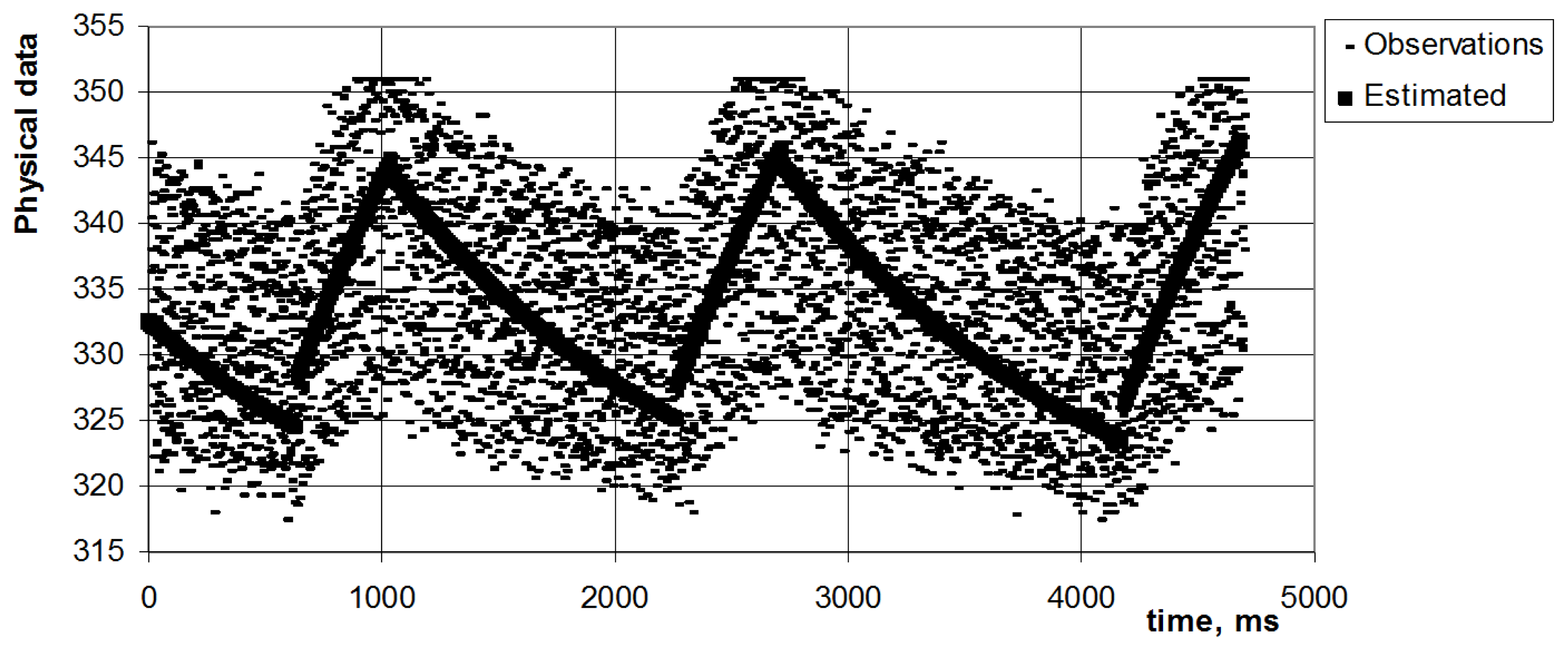
A toy numeric example with a control signal perturbing a first order nonhomogenous ordinary differential equation system by a relay control (on/off or so-called bang-bang control) is shown below. This type of control signal causes a discontinuity point in the domain of the differential equations system. Simultaneous inferring of the differential equation parameters is illustrated.

If the measured time series is in a vector form, cx_k, i.e., at time moments t₀, t₁, ..., t_n observations (data) are collected regarding the one dimensional variable x(t) as cx₀, cx₁, ..., cx_n, then our entropy will have the form,

$$S(P,P_{likelihood})=-\sum _{k=1}^n\underset{-\infty }{\overset{\infty }{\int }}\cdots \underset{-\infty }{\overset{\infty }{\int }}P(\langle {\mathbf{x}}_k\rangle ,{\mathbf{x}}_k)·\text{log\hspace{0.17em}}\left(\frac{P(\langle {\mathbf{x}}_k\rangle ,{\mathbf{x}}_k)}{P_{likelihood}(\mathbf{c}{\mathbf{x}}_k,{\mathbf{x}}_k)}\right)\hspace{0.17em}\text{d}{\mathbf{x}}_k,$$

(3)

where the posterior distribution, P = P (〈x_k〉, x_k), would update the prior distribution, P_likelihood (cx_k, x_k), so that our set of estimated values for 〈x_k〉 maximizes the entropy; Equation (3). This enforces the constraints in Equation (2) on the posterior and produces a Lagrangian,

$$L(P,P_{likelihood})=-\sum _{k=1}^n\underset{-\infty }{\overset{\infty }{\int }}\cdots \underset{-\infty }{\overset{\infty }{\int }}P(\langle {\mathbf{x}}_k\rangle ,{\mathbf{x}}_k)·\text{log\hspace{0.17em}}\left(\frac{P(\langle {\mathbf{x}}_k\rangle ,{\mathbf{x}}_k)}{P_{likelihood}(\mathbf{c}{\mathbf{x}}_k,{\mathbf{x}}_k)}\right)\hspace{0.17em}\text{d}{\mathbf{x}}_k+\sum _{k=1}^n{\lambda }_k·f(\langle {\mathbf{x}}_k\rangle ,\mathit{\delta },{\mathbf{u}}_k).$$

(4)

The integral Equation (4) can be multidimensional. Furthermore, the exact form of the constraints may be unknown or so-called non-parametric, i.e., their behavior is known, but the constraints’ forms or mathematical models are undefined. Integrals should be summed over time windows to establish a Lagrangian for the joint action in such cases. One should consider using the computationally feasible methods of the Monte Carlo family or similar brute force sampling approaches for these cases. In our toy example, an example with a computable solution is provided, and other complicated cases are out of the scope of the paper.

In some cases, Equation (4) does not have a closed form solution, and one should seek a numeric iterative approach. For example, when the mathematical models are parabolic partial differential equations, applying the variational data assimilation method as in [11] is suggested. In our toy example, Equation (4) has a closed form solution with some unknown parameters from our mathematical model. These parameters are inferred by using boundary conditions, which are satisfied for the time series. If it is assumed that the control signal that perturbs the system is known and it is further assumed that there are two subsequent sets of time series with different perturbations, then one approach to explicitly estimate the value of the unknown parameter δ is to find it, such that it satisfies the boundary condition between the two time series, i.e., the last estimate of the first time series must be equal to the very first estimate of the next time series. This is illustrated in the following section, where this is accomplished by incorporating the differential equation’s boundary condition.

2.2. Example with Nonhomogenous Differential Equation Constraints

We examine a toy system below that uses a one-dimensional time series of measurements. At time moments t₀, t₁, ..., t_n observations (data) are collected regarding the one-dimensional variable x(t) as cx₀, cx₁, ..., cx_n. We assume the observations are represented by independent probabilistic variables x₀, x₁, ..., x_n, and their uncertainties are equal to ${\sigma }_{cx}^2$. Then, the probability density function of the joint prior or the likelihood [2] for the time series variables is,

$$P_{likelihood}(x_0,\dots ,x_n)=\frac{1}{{\left(\sqrt{2\pi {\sigma }_{cx}^2}\right)}^{n+1}}\text{exp\hspace{0.17em}}\left[-\frac{1}{2{\sigma }_{cx}^2}\sum _{k=0}^n{(x_k-c{x}_k)}^2\right].$$

(5)

Note: It is reasonable to see the likelihood as containing “prior” information, since it represents the relationship that has already been established between observation values and probabilistic variables.

The goal here is to find a posterior distribution for the variables that will satisfy the constraints (dynamics). Frequently, the unbiased model is unknown for the variable as a function of time, because it contains unobservable nonlinearities. Further, the analytical closed form model can be more complicated than what is known a priori about the system based on experience. Yet, often, the main behavior of a system can be approximated by an exponential law. Thus, inferring the posterior distribution may be done by not incorporating the dynamic constraints, which exactly represent the physical system behavior, but by the constraints representing an exponential approximation. This type of assumption that uses an exponential approximation allows for the closed form solutions to be found for practical filtering applications and will be shown below, e.g., simultaneously approximating a time series with an exponential curve, while inferring parameters of the differential equation.

The main problem with the estimation of an exponential mathematical model is that the start and the end processes, and thus, the data from them, are equally important. Markov assumptions cannot then be explicitly assumed. In the resistance-inductance (RL) circuit, where the control signal is the voltage signal for the circuit, the parameters (R and L) of the circuit can be calculated from the transient conditions when a step control signal function is applied and the system is in a steady state. At the beginning, the rate of current increase will give information about the inertia of the system, which is represented by L. At the end of the transient process, the steady state of the system will give information about the resistance of the system R. Thus, the time series is “smoothed” with an approximate exponential law, and the estimates must be determined with a wide enough processing window that not only covers the start of the transient process, but also so that the pattern of the saturation effect is partially “seen” in the time series. This way, the estimates, which behave according to the exponential law, as well as the parameters of the differential equation are inferred. In other words, the more information that is included, the less uncertainty is left in the estimate expression after the entropy is maximized.

Again, for illustration, assume that the following approximation for the system behavior model is,

$$u(t)=\delta ·(x(t)-x_{steady})+C·\frac{\text{d}x(t)}{\text{d}t},$$

(6)

where u (t) is the control signal that perturbs the system variable, x(t), according to Equation (6), and where δ and C are the parameters of the first order nonhomogenous, differential equation and x_steady is the steady state value of the variable x(t) when there is no control signal u (t) applied, assuming that the system is in a steady state. Further, it can be assumed that the system control signal, u(t), is constant over the duration of all discretization intervals, Δt, at any time moment k. It can also be assume that Equation (6) is the constraint over the probabilistic variable’s mean. In this case, the constraint is,

$$u(t)=\delta ·(\langle x(t)\rangle -x_{steady})+C·\frac{\text{d}\langle x(t)\rangle }{\text{d}t}.$$

(7)

Here, the mean of some probabilistic variable is a function of time. The inference process should not only estimate the means of the probabilistic variable at time moments k, but also take into account the dynamics, which is given a priori. The solution of Equation (6) is represented by,

$$\langle x(t)\rangle =\frac{u}{\delta }+x_{steady}-\left(\frac{u}{\delta }+x_{steady}-x_0\right)·\text{exp\hspace{0.17em}}\left(-\frac{\delta ·\mathrm{\Delta }t}{C}\right),$$

(8)

where x₀ represents the initial condition value at some initial time. If it is assumed that the initial conditions of the variable x(t) are the previous sample’s value and the current sample’s value is the final value after the discretization interval passed, then Equation (8) can be rewritten as:

$$\langle x_k\rangle =\frac{u}{\delta }+x_{steady}-\left(\frac{u}{\delta }+x_{steady}-\langle x_{k-1}\rangle \right)·\text{exp\hspace{0.17em}}\left(-\frac{\delta ·\mathrm{\Delta }t}{C}\right).$$

(9)

The exponential term does not depend on the actual means, so an intermediate notation will used, $\gamma (\delta )\equiv \text{exp\hspace{0.17em}}\left(-\frac{\delta ·\mathrm{\Delta }t}{C}\right)$, which simplifies the expression to,

$$\langle x_k\rangle =\frac{u}{\delta }+x_{steady}-\left(\frac{u}{\delta }+x_{steady}-\langle x_{k-1}\rangle \right)·\gamma (\delta ).$$

(10)

The common denominator is found, and all of the terms to the left side of Equation (10) are moved, which yields,

$$\delta ·\langle x_k\rangle -u-\delta ·x_{steady}+(u+\delta ·(x_{steady}-\langle x_{k-1}\rangle ))·\gamma (\delta )=0,$$

(11)

The entropy is maximized to find the joint distribution that is closest to P_obs, but that also satisfies the approximate model (knowledge about the system) in Equation (9), which is assumed is enough to mimic the behavior of the system at the a macroscopic level. Before doing so, the general shape of the posterior distribution will be assumed, but the scaling factors are unknown, so that,

$$P_{posterior}(x_0,\dots ,x_n)=\frac{1}{{\left(\sqrt{2\pi {\sigma }_{\langle x\rangle }^2}\right)}^{n+1}}\text{exp\hspace{0.17em}}\left[-\frac{1}{2{\sigma }_{\langle x\rangle }^2}\sum _{k=0}^n{(x_k-\langle x_k\rangle )}^2\right],$$

(12)

where it is assumed that the variance of the means ${\sigma }_{\langle x\rangle }^2$ is constant for each variable, respectively, for illustrative purposes. Then, the entropy to be maximized is,

$$S(P_{posterior},P_{likelihood})=-\sum _{k=0}^n\underset{-\infty }{\overset{\infty }{\int }}\cdots \underset{-\infty }{\overset{\infty }{\int }}{P}_{posterior}(x_0,\dots ,x_n)·\text{log\hspace{0.17em}}\left(\frac{P_{posterior}(x_0,\dots ,x_n)}{P_{likelihood}(x_0,\dots ,x_n)}\right)\hspace{0.17em}\text{d}\mathrm{\Omega }.$$

(13)

This is maximized to derive the Lagrangian,

$$\begin{array}{l}L(P_{posterior},P_{likelihood})=-\sum _{k=0}^n\underset{-\infty }{\overset{\infty }{\int }}\cdots \underset{-\infty }{\overset{\infty }{\int }}{P}_{posterior}(x_0,\dots ,x_n)·\text{log\hspace{0.17em}}\left(\frac{P_{posterior}(x_0,\dots ,x_n)}{P_{likelihood}(x_0,\dots ,x_n)}\right)\hspace{0.17em}\text{d}\mathrm{\Omega }\\ +\sum _{k=1}^n{\lambda }_k·(\delta ·\langle x_k\rangle -u-\delta ·x_{steady}+(u+\delta ·(x_{steady}-\langle x_{k-1}\rangle ))·\gamma (\delta )),\end{array}$$

(14)

where dΩ = dx₀ · dx₁ · . . . · dx_k · . . . · dx_n and where λ_k are the Lagrange multipliers, which enforce the constraints (dynamics) over the means of the variables under consideration. By inserting Equations (5) and (12) into Equation (14) and integrating over the variables, the Lagrangian is simplified to,

$$\begin{array}{l}{L}_s(P_{posterior},P_{likelihood})=\sum _{k=0}^n{(c{x}_k-\langle x_k\rangle )}^2+\varepsilon \\ +\sum _{k=1}^n{\lambda }_k·(\delta ·\langle x_k\rangle -u-\delta ·x_{steady}+(u+\delta ·(x_{steady}-\langle x_{k-1}\rangle ))·\gamma (\delta )),\end{array}$$

(15)

where ε is an integration constant along with additive terms, which do not affect the Lagrangian in Equation (15). This constant can be omitted, which yields the final Lagrangian,

$$\begin{array}{l}{L}_s(P_{posterior},P_{likelihood})=\sum _{k=0}^n{(c{x}_k-\langle x_k\rangle )}^2\\ +\sum _{k=1}^n{\lambda }_k·(\delta ·\langle x_k\rangle -u-\delta ·x_{steady}+(u+\delta ·(x_{steady}-\langle x_{k-1}\rangle ))·\gamma (\delta )),\end{array}$$

(16)

It should be noted at this point that the “distance” that is mentioned in [10] is the quadratic term in the Lagrangian.

2.3. Maximization of the Expectation

After differentiating the entropy with respect to the variables means, 〈x₀〉, . . ., 〈x_n〉, a system of n+1 equations is formed,

$$\{\begin{array}{r}\hfill 2·\langle x_0\rangle -2·c{x}_0-\gamma (\delta )·\delta ·{\lambda }_1=0;\\ \hfill 2·\langle x_1\rangle -2·c{x}_1+\delta ·({\lambda }_1-\gamma (\delta )·{\lambda }_2)=0;\\ \hfill \cdots \\ \hfill 2·\langle x_n-1\rangle -2·c{x}_{n-1}+\delta ·({\lambda }_{n-1}-\gamma (\delta )·{\lambda }_n)=0;\\ \hfill 2·\langle x_n\rangle -2·c{x}_n-\delta ·{\lambda }_n)=0.\end{array}$$

(17)

Every discretization interval constraint (which originates from Equation (11) forms the system of n equations,

$$\{\begin{array}{c}\delta ·\langle x_1\rangle -u-\delta ·x_{steady}+(u+\delta ·(x_{steady}-\langle x_0\rangle ))·\gamma (\delta )=0;\\ \cdots \\ \delta ·\langle x_k\rangle -u-\delta ·x_{steady}+(u+\delta ·(x_{steady}-\langle x_{k-1}\rangle ))·\gamma (\delta )=0;\\ \cdots \\ \delta ·\langle x_n\rangle -u-\delta ·x_{steady}+(u+\delta ·(x_{steady}-\langle x_{n-1}\rangle ))·\gamma (\delta )=0,\end{array}$$

(18)

which together with Equation (17) form a system of 2n + 1 linear equations that have a closed form solution.

For illustration, the solutions for the cases n = 4, n = 6 and n = 8 are provided. After this is done, the pattern of the solution will be generalized.

In the first case (n = 4), the function f is differentiable. For illustration, we assume that there are jump discontinuities at discretization points x₀, x₄, x₈, x₁₂, etc. It is not a necessity to strictly enforce this assumption, but it is made so that the sequence of actions necessary for this approach are clear. At the jump discontinuities in this system (control signal in the whole period of the differentiable interval is constant), the boundary conditions claim that 〈x_k (−0)〉 = 〈x_k (+0)〉, i.e., the boundary condition is of the Dirichlet type. Then, for every differentiable period of the function, we have two systems of equations,

$$\{\begin{array}{r}\hfill 2·\langle x_0\rangle -2·c{x}_0-\gamma (\delta )·\delta ·{\lambda }_1=0;\\ \hfill 2·\langle x_1\rangle -2·c{x}_1+\delta ·({\lambda }_1-\gamma (\delta )·{\lambda }_2)=0;\\ \hfill 2·\langle x_2\rangle -2·c{x}_2+\delta ·({\lambda }_2-\gamma (\delta )·{\lambda }_3)=0;\\ \hfill 2·\langle x_3\rangle -2·c{x}_3+\delta ·({\lambda }_3-\gamma (\delta )·{\lambda }_4)=0;\\ \hfill 2·\langle x_4\rangle -2·c{x}_4-\delta ·{\lambda }_4)=0,\end{array}$$

(19)

and:

$$\{\begin{array}{l}\delta ·\langle x_1\rangle -u-\delta ·x_{steady}+(u+\delta ·(x_{steady}-\langle x_0\rangle ))·\gamma (\delta )=0;\hfill \\ \delta ·\langle x_2\rangle -u-\delta ·x_{steady}+(u+\delta ·(x_{steady}-\langle x_1\rangle ))·\gamma (\delta )=0;\hfill \\ \delta ·\langle x_3\rangle -u-\delta ·x_{steady}+(u+\delta ·(x_{steady}-\langle x_2\rangle ))·\gamma (\delta )=0;\hfill \\ \delta ·\langle x_4\rangle -u-\delta ·x_{steady}+(u+\delta ·(x_{steady}-\langle x_3\rangle ))·\gamma (\delta )=0,\hfill \end{array}$$

(20)

which results in to a system of nine equations and mine unknowns consisting of five state variables and four Lagrange multipliers,

$$\{\begin{array}{r}\hfill 2·\langle x_0\rangle -2·c{x}_0-\gamma (\delta )·\delta ·{\lambda }_1=0;\\ \hfill 2·\langle x_1\rangle -2·c{x}_1+\delta ·({\lambda }_1-\gamma (\delta )·{\lambda }_2)=0;\\ \hfill 2·\langle x_2\rangle -2·c{x}_2+\delta ·({\lambda }_2-\gamma (\delta )·{\lambda }_3)=0;\\ \hfill 2·\langle x_3\rangle -2·c{x}_3+\delta ·({\lambda }_3-\gamma (\delta )·{\lambda }_4)=0;\\ \hfill 2·\langle x_4\rangle -2·c{x}_4-\delta ·{\lambda }_4=0;\\ \hfill \delta ·\langle x_1\rangle -u-\delta ·x_{steady}+(u+\delta ·(x_{steady}-\langle x_0\rangle ))·\gamma (\delta )=0;\\ \hfill \delta ·\langle x_2\rangle -u-\delta ·x_{steady}+(u+\delta ·(x_{steady}-\langle x_1\rangle ))·\gamma (\delta )=0;\\ \hfill \delta ·\langle x_3\rangle -u-\delta ·x_{steady}+(u+\delta ·(x_{steady}-\langle x_2\rangle ))·\gamma (\delta )=0;\\ \hfill \delta ·\langle x_4\rangle -u-\delta ·x_{steady}+(u+\delta ·(x_{steady}-\langle x_3\rangle ))·\gamma (\delta )=0.\end{array}$$

(21)

After some manipulations, the final solution for the two state variables 〈x₀〉 and 〈x₄〉 is:

$$\begin{array}{l}\langle x_0\rangle =c{x}_0·\frac{1}{1+\gamma {(\delta )}^2+\gamma {(\delta )}^4+\gamma {(\delta )}^6+\gamma {(\delta )}^8}\\ +c{x}_1·\frac{\gamma (\delta )}{1+\gamma {(\delta )}^2+\gamma {(\delta )}^4+\gamma {(\delta )}^6+\gamma {(\delta )}^8}+c{x}_2·\frac{\gamma {(\delta )}^2}{1+\gamma {(\delta )}^2+\gamma {(\delta )}^4+\gamma {(\delta )}^6+\gamma {(\delta )}^8}\\ +c{x}_3·\frac{\gamma {(\delta )}^3}{1+\gamma {(\delta )}^2+\gamma {(\delta )}^4+\gamma {(\delta )}^6+\gamma {(\delta )}^8}+c{x}_4·\frac{\gamma {(\delta )}^4}{1+\gamma {(\delta )}^2+\gamma {(\delta )}^4+\gamma {(\delta )}^6+\gamma {(\delta )}^8}\\ -\left(\frac{u}{\delta }+x_{steady}\right)·\frac{-\gamma (\delta )+\gamma {(\delta )}^2-\gamma {(\delta )}^3+\gamma {(\delta )}^4}{1-\gamma (\delta )+\gamma {(\delta )}^2-\gamma {(\delta )}^3+\gamma {(\delta )}^4},\end{array}$$

(22)

and:

$$\begin{array}{l}\langle x_4\rangle =c{x}_0·\frac{\gamma {(\delta )}^4}{1+\gamma {(\delta )}^2+\gamma {(\delta )}^4+\gamma {(\delta )}^6+\gamma {(\delta )}^8}\\ +c{x}_1·\frac{\gamma {(\delta )}^5}{1+\gamma {(\delta )}^2+\gamma {(\delta )}^4+\gamma {(\delta )}^6+\gamma {(\delta )}^8}+c{x}_2·\frac{\gamma {(\delta )}^6}{1+\gamma {(\delta )}^2+\gamma {(\delta )}^4+\gamma {(\delta )}^6+\gamma {(\delta )}^8}\\ +c{x}_3·\frac{\gamma {(\delta )}^7}{1+\gamma {(\delta )}^2+\gamma {(\delta )}^4+\gamma {(\delta )}^6+\gamma {(\delta )}^8}+c{x}_4·\frac{\gamma {(\delta )}^8}{1+\gamma {(\delta )}^2+\gamma {(\delta )}^4+\gamma {(\delta )}^6+\gamma {(\delta )}^8}\\ -\left(\frac{u}{\delta }+x_{steady}\right)·\frac{-\gamma (\delta )+\gamma {(\delta )}^2-\gamma {(\delta )}^3+\gamma {(\delta )}^4}{1-\gamma (\delta )+\gamma {(\delta )}^2-\gamma {(\delta )}^3+\gamma {(\delta )}^4}.\end{array}$$

(23)

Values 〈x₀〉 and 〈x₄〉 belong to the very first differentiable period of the time series when a control signal u is a constant, i.e., u_first = const. Thus, the closed form solutions for〈x₀ (+0)〉 and 〈x₄ (−0)〉 values have been found.

After introducing the following coefficients for convenience,

$${\alpha }_k=\frac{\gamma {(\delta )}^k}{{\displaystyle \sum _{i=0}^{n=4}}\gamma {(\delta )}^{2i}},$$

(24)

$${\beta }_0=\frac{{\displaystyle \sum _{i=1}^{n=4}}{(-1)}^i\gamma {(\delta )}^i}{{\displaystyle \sum _{i=0}^{n=4}}{(-1)}^i\gamma {(\delta )}^i},$$

(25)

$${\beta }_4=\frac{{\displaystyle \sum _{i=0}^{n-1=3}}{(-1)}^i\gamma {(\delta )}^i}{{\displaystyle \sum _{i=0}^{n=4}}{(-1)}^i\gamma {(\delta )}^i},$$

(26)

and Equations (22) and (23) can be written as,

$$\langle x_0(+0)\rangle =c{x}_0·{\alpha }_0+c{x}_1·{\alpha }_1+c{x}_2·{\alpha }_2+c{x}_3·{\alpha }_3+c{x}_4·{\alpha }_4-\left(\frac{u_{first}}{\delta }+x_{steady}\right)·{\beta }_0,$$

(27)

$$\langle x_4(-0)\rangle =c{x}_0·{\alpha }_4+c{x}_1·{\alpha }_5+c{x}_2·{\alpha }_6+c{x}_3·{\alpha }_7+c{x}_4·{\alpha }_8-\left(\frac{u_{first}}{\delta }+x_{steady}\right)·{\beta }_4.$$

(28)

For this first differentiable period, the coefficients effective at the jump discontinuity of the control signal from u_first to u_second at the fourth discretization interval are introduced,

$$A_{first}=c{x}_0·{\alpha }_0+c{x}_1·{\alpha }_1+c{x}_2·{\alpha }_2+c{x}_3·{\alpha }_3+c{x}_4·{\alpha }_4-x_{steady}·{\beta }_0,$$

(29)

$$B_{first}=-u_{first}·{\beta }_4.$$

(30)

The expression of 〈x₄ (−0)〉 can be rewritten as:

$$\langle x_4(-0)\rangle =A_{first}+\frac{B_{first}}{\delta }.$$

(31)

The next differentiable period from the fourth to eight discretization intervals, where again we have n = 4 (this is not necessary, but the same value is used for illustration purposes). This yields the closed form expressions for the state variables at the jump discontinuities,

$$\langle x_4(+0)\rangle =c{x}_4·{\alpha }_0+c{x}_5·{\alpha }_1+c{x}_6·{\alpha }_2+c{x}_7·{\alpha }_3+c{x}_8·{\alpha }_4-\left(\frac{u_{\text{sec}ond}}{\delta }+x_{steady}\right)·{\beta }_0,$$

(32)

$$\langle x_8(-0)\rangle =c{x}_4·{\alpha }_4+c{x}_5·{\alpha }_5+c{x}_6·{\alpha }_6+c{x}_7·{\alpha }_7+c{x}_8·{\alpha }_8-\left(\frac{u_{\text{sec}ond}}{\delta }+x_{steady}\right)·{\beta }_4.$$

(33)

After introducing convenience coefficients for 〈x₄ (+0)〉,

$$A_{second}=c{x}_4·{\alpha }_4+c{x}_5·{\alpha }_5+c{x}_6·{\alpha }_6+c{x}_7·{\alpha }_7+c{x}_8·{\alpha }_8-x_{steady}·{\beta }_0,$$

(34)

$$B_{second}=-u_{second}·{\beta }_4,$$

(35)

the expression for 〈x₄ (+0)〉 is arrived at,

$$\langle x_4(+0)\rangle =A_{second}+\frac{B_{second}}{\delta }.$$

(36)

From a macroscopic level, there is a Dirichlet boundary condition with jump discontinuity at the fourth discretization interval, which states that 〈x₄ (−0)〉 = 〈x₄ (+0)〉. The following equation is solved to determine δ,

$$A_{first}+\frac{B_{first}}{\delta }=A_{second}+\frac{B_{second}}{\delta }$$

(37)

which yields,

$$\delta =\frac{B_{second}-B_{first}}{A_{first}-A_{second}}.$$

(38)

One might ask: if the illustrative coefficients A_first, B_first, A_second and B_second that were selected are all functions of δ, then is the calculation of Equation (38) valid? Generally not if the rate of change of δ is of the same order as the discretization interval’s size. For this example, it is a priori known that some external disturbances affect our system through changing the value of δ, i.e., it is actually a function of time, δ (t). However, in many physical systems, the parameters’ rate of change is much smaller than the rates of change of the state and control variables. Specifically, in a current application of this, the rate of change of δ (t) in our system was ten-times smaller than the duration of differentiable period. This allowed us to assume that γ(δ) was constant, because any change in δ resulted in approximately a ten- to one hundred-times smaller change in γ(δ) compared to the change effecting Equation (37). Therefore, the algorithm can start from a certain value of δ, find the δ using Equation (38), then put it back into expressions Equations (24)–(31), with the recalculated estimates of the means at the boundary condition defined by discontinuity point. Normally, after 3–5 iterations, the value of δ converges to the acceptable precision.

When δ converges to an acceptable value, the remaining estimates of, 〈x₁〉, 〈x₂〉 and 〈x₃〉 are calculated. Thus, some information from observations is precalculated and then applied to the boundary conditions. This yields the exact values for the differentiable points, which are in between the discontinuity points.

Let us analyze the example with n = 6. Similarly to previous example, we derive our boundary solution for the system of 13 equations as,

$$\begin{array}{l}\langle x_0\rangle =c{x}_0·\frac{1}{1+\gamma {(\delta )}^2+\gamma {(\delta )}^4+\gamma {(\delta )}^6+\gamma {(\delta )}^8+\gamma {(\delta )}^{10}+\gamma {(\delta )}^{12}}\\ +c{x}_1·\frac{\gamma (\delta )}{1+\gamma {(\delta )}^2+\gamma {(\delta )}^4+\gamma {(\delta )}^6+\gamma {(\delta )}^8+\gamma {(\delta )}^{10}+\gamma {(\delta )}^{12}}+c{x}_2·\frac{\gamma {(\delta )}^2}{1+\gamma {(\delta )}^2+\gamma {(\delta )}^4+\gamma {(\delta )}^6+\gamma {(\delta )}^8+\gamma {(\delta )}^{10}+\gamma {(\delta )}^{12}}\\ +c{x}_3·\frac{\gamma {(\delta )}^3}{1+\gamma {(\delta )}^2+\gamma {(\delta )}^4+\gamma {(\delta )}^6+\gamma {(\delta )}^8+\gamma {(\delta )}^{10}+\gamma {(\delta )}^{12}}+c{x}_4·\frac{\gamma {(\delta )}^4}{1+\gamma {(\delta )}^2+\gamma {(\delta )}^4+\gamma {(\delta )}^6+\gamma {(\delta )}^8+\gamma {(\delta )}^{10}+\gamma {(\delta )}^{12}}\\ +c{x}_5·\frac{\gamma {(\delta )}^5}{1+\gamma {(\delta )}^2+\gamma {(\delta )}^4+\gamma {(\delta )}^6+\gamma {(\delta )}^8+\gamma {(\delta )}^{10}+\gamma {(\delta )}^{12}}+c{x}_6·\frac{\gamma {(\delta )}^6}{1+\gamma {(\delta )}^2+\gamma {(\delta )}^4+\gamma {(\delta )}^6+\gamma {(\delta )}^8+\gamma {(\delta )}^{10}+\gamma {(\delta )}^{12}}\\ -\left(\frac{u}{\delta }+x_{steady}\right)·\frac{-\gamma (\delta )+\gamma {(\delta )}^2-\gamma {(\delta )}^3+\gamma {(\delta )}^4-\gamma {(\delta )}^5+\gamma {(\delta )}^6}{1-\gamma (\delta )+\gamma {(\delta )}^2-\gamma {(\delta )}^3+\gamma {(\delta )}^4-\gamma {(\delta )}^5+\gamma {(\delta )}^6},\end{array}$$

(39)

$$\begin{array}{l}\langle x_6\rangle =c{x}_0·\frac{\gamma {(\delta )}^6}{1+\gamma {(\delta )}^2+\gamma {(\delta )}^4+\gamma {(\delta )}^6+\gamma {(\delta )}^8+\gamma {(\delta )}^{10}+\gamma {(\delta )}^{12}}\\ +c{x}_1·\frac{\gamma {(\delta )}^7}{1+\gamma {(\delta )}^2+\gamma {(\delta )}^4+\gamma {(\delta )}^6+\gamma {(\delta )}^8+\gamma {(\delta )}^{10}+\gamma {(\delta )}^{12}}+c{x}_2·\frac{\gamma {(\delta )}^8}{1+\gamma {(\delta )}^2+\gamma {(\delta )}^4+\gamma {(\delta )}^6+\gamma {(\delta )}^8+\gamma {(\delta )}^{10}+\gamma {(\delta )}^{12}}\\ +c{x}_3·\frac{\gamma {(\delta )}^9}{1+\gamma {(\delta )}^2+\gamma {(\delta )}^4+\gamma {(\delta )}^6+\gamma {(\delta )}^8+\gamma {(\delta )}^{10}+\gamma {(\delta )}^{12}}+c{x}_4·\frac{\gamma {(\delta )}^{10}}{1+\gamma {(\delta )}^2+\gamma {(\delta )}^4+\gamma {(\delta )}^6+\gamma {(\delta )}^8+\gamma {(\delta )}^{10}+\gamma {(\delta )}^{12}}\\ +c{x}_5·\frac{\gamma {(\delta )}^{11}}{1+\gamma {(\delta )}^2+\gamma {(\delta )}^4+\gamma {(\delta )}^6+\gamma {(\delta )}^8+\gamma {(\delta )}^{10}+\gamma {(\delta )}^{12}}+c{x}_6·\frac{\gamma {(\delta )}^{12}}{1+\gamma {(\delta )}^2+\gamma {(\delta )}^4+\gamma {(\delta )}^6+\gamma {(\delta )}^8+\gamma {(\delta )}^{10}+\gamma {(\delta )}^{12}}\\ -\left(\frac{u}{\delta }+x_{steady}\right)·\frac{-\gamma (\delta )+\gamma {(\delta )}^2-\gamma {(\delta )}^3+\gamma {(\delta )}^4-\gamma {(\delta )}^5+\gamma {(\delta )}^6}{1-\gamma (\delta )+\gamma {(\delta )}^2-\gamma {(\delta )}^3+\gamma {(\delta )}^4-\gamma {(\delta )}^5+\gamma {(\delta )}^6}.\end{array}$$

(40)

The convenience coefficients are then redefined as:

$${\alpha }_k=\frac{\gamma {(\delta )}^k}{{\displaystyle \sum _{i=0}^{n=6}}\gamma {(\delta )}^{2i}},{\beta }_0=\frac{{\displaystyle \sum _{i=1}^{n=6}}{(-1)}^i\gamma {(\delta )}^i}{{\displaystyle \sum _{i=0}^{n=6}}{(-1)}^i\gamma {(\delta )}^i},{\beta }_6=\frac{{\displaystyle \sum _{i=0}^{n-1=5}}{(-1)}^i\gamma {(\delta )}^i}{{\displaystyle \sum _{i=0}^{n=6}}{(-1)}^i\gamma {(\delta )}^i},$$

(41)

which yields,

$$A_{first}=c{x}_0·{\alpha }_0+c{x}_1·{\alpha }_1+c{x}_2·{\alpha }_2+c{x}_3·{\alpha }_3+c{x}_4·{\alpha }_4+c{x}_5·{\alpha }_5+c{x}_6·{\alpha }_6-x_{steady}·{\beta }_0,$$

(42)

$$B_{first}=-u_{first}·{\beta }_6,$$

(43)

$$A_{second}=c{x}_6·{\alpha }_6+c{x}_7·{\alpha }_7+c{x}_8·{\alpha }_8+c{x}_9·{\alpha }_9+c{x}_{10}·{\alpha }_{10}+c{x}_{11}·{\alpha }_{11}+c{x}_{12}·{\alpha }_{12}-x_{steady}·{\beta }_0,$$

(44)

$$B_{second}=-u_{second}·{\beta }_6.$$

(45)

The δ is determined by the same procedure with the 3–5 iterations that were used with Equation (38) and n = 4.

For the third example of n = 8, the convenience coefficients that are affected are only shown,

$${\alpha }_k=\frac{\gamma {(\delta )}^k}{{\displaystyle \sum _{i=0}^{n=8}}\gamma {(\delta )}^{2i}},{\beta }_0=\frac{{\displaystyle \sum _{i=1}^{n=8}}{(-1)}^i\gamma {(\delta )}^i}{{\displaystyle \sum _{i=0}^{n=8}}{(-1)}^i\gamma {(\delta )}^i},{\beta }_8=\frac{{\displaystyle \sum _{i=0}^{n-1=7}}{(-1)}^i\gamma {(\delta )}^i}{{\displaystyle \sum _{i=0}^{n=8}}{(-1)}^i\gamma {(\delta )}^i},$$

(46)

which yields,

$$\begin{array}{l}{A}_{first}=c{x}_0·{\alpha }_0+c{x}_1·{\alpha }_1+c{x}_2·{\alpha }_2+c{x}_3·{\alpha }_3+c{x}_4·{\alpha }_4\\ +c{x}_5·{\alpha }_5+c{x}_6·{\alpha }_6+c{x}_7·{\alpha }_7+c{x}_8·{\alpha }_8-x_{steady}·{\beta }_0,\end{array}$$

(47)

$$B_{first}=-u_{first}·{\beta }_8,$$

(48)

$$\begin{array}{l}{A}_{second}=c{x}_8·{\alpha }_8+c{x}_9·{\alpha }_9+c{x}_{10}·{\alpha }_{10}+c{x}_{11}·{\alpha }_{11}+c{x}_{12}·{\alpha }_{12}+\\ +c{x}_{13}·{\alpha }_{13}+c{x}_{14}·{\alpha }_{14}+c{x}_{15}·{\alpha }_{15}+c{x}_{16}·{\alpha }_{16}-x_{steady}·{\beta }_0,\end{array}$$

(49)

$$B_{second}=-u_{second}·{\beta }_8.$$

(50)

2.4. Generalization of the Estimation Algorithm

After seeing the pattern of solutions in Equations (47)–(50), we generalize for any even number, n discretization intervals of the differentiable period. The convenience coefficients are redefined for the solution pattern,

$${\alpha }_k=\frac{\gamma {(\delta )}^k}{{\displaystyle \sum _{i=0}^n}\gamma {(\delta )}^{2i}},$$

(51)

$${\beta }_0=\frac{{\displaystyle \sum _{i=1}^n}{(-1)}^i\gamma {(\delta )}^i}{{\displaystyle \sum _{i=0}^n}{(-1)}^i\gamma {(\delta )}^i},$$

(52)

$${\beta }_n=\frac{{\displaystyle \sum _{i=0}^{n-1}}{(-1)}^i\gamma {(\delta )}^i}{{\displaystyle \sum _{i=0}^n}{(-1)}^i\gamma {(\delta )}^i}.$$

(53)

The mean estimate expressions for the boundary conditions, i.e., for the first 〈x₀ (+0)〉 and the last 〈x_n (−0)〉 means of the time series are as follows,

$$\langle x_0(-0)\rangle =\sum _{i=0}^n{\alpha }_k·c{x}_k-\frac{{\beta }_0·u}{\delta }-{\beta }_0·x_{steady},$$

(54)

and:

$$\langle x_n(+0)\rangle =\sum _{i=0}^n{\alpha }_{k+n}·c{x}_k-\frac{{\beta }_n·u}{\delta }-{\beta }_n·x_{steady}.$$

(55)

The value of the parameter γ(δ) is not affected by the change in δ nearly as much as the effect that δ produces in equation Equations (54) and (55). This is because the discretization interval, Δt, is usually chosen as small as possible (typically limited by embedded hardware resources), and the total duration of the time series (the processing window of simultaneous updates or the part of f of differentiable points) is also relatively small. Different control signals u_first and u_second for two subsequent time series with jump discontinuities between, δ, can be calculated based on the fact that the last estimated mean of the first processing window is equal to the first estimated mean of the next processing window. In other words, if Equations (54) and (55) can be rewritten into the form,

$$\langle x_n(-0)\rangle =A_{first}+\frac{B_{first}}{\delta },$$

(56)

and:

$$\langle x_n(+0)\rangle =A_{second}+\frac{B_{second}}{\delta },$$

(57)

where 〈x_n (−0)〉 = 〈x_n (+0)〉. The value for δ is found using Equation (38). After the estimate for δ is determined from Equation (38), the parameter γ can be recalculated and then used to calculate the mean estimates according to the expression in Equations (54) and (55) again; and then, calculate δ again by using Equation (38), and so on. This algorithm usually requires 3–5 iterations to converge to the acceptable precision of δ, regardless of the uncertainty of the input variables. Acceptable precision in our case is the situation when a new iteration changed the δ value by 0.1%. At this point, we assume that it is no longer necessary to proceed with further iterations, because the information gain about the value would become negligible.

We present the algorithm for the calculation in pseudo code:

double Calculate Delta Coefficient (
               double initial value,
               double precision,
               double [] observations,
               double C, // inertia coefficient as constant
               double u, // control signal’ s value
               double x_steady, // steady state value
               double dt // the size of discretization interval
{
               double delta = initial_value;
               double earlier_delta = undefined;
               precalculate arguments of equations containing
                            a) observations;
                            b) coefficient C;
                            c) the size of discretization interval;
                            d) control signals value;
                            e) steady state value of variable;
               while (true) // loop continuously
               {
                            calculate alpha and beta coefficients;
                            calculate A_first, B_first, A_sec, B_sec;
                            delta = (B_sec – B_first)/(A_first – A_sec);
                            if ((delta – earlier_delta )ˆ2< precision)
                                         break ; // halt the loop
                            earlier_delta = delta;
               }
               return delta;
}

Notice that there is still a singular point in Equation (38) that has to be avoided when implementing the filtering algorithm. The coefficients A_first and A_second depend on the observation values, as shown in Equations (54) and (55). Thus, the size of n needs to be such that the change in observations in the processing window is noticeable in order to avoid this singularity in a real system, i.e., the system must be perturbed enough or its control signal is reduced so that the change of measurements of the input channel is noticeable. If this condition is satisfied, the MrE filter will be stable. Our physical system naturally satisfied this requirement. In this example, during the whole measurement and estimation process, there are no singularities.

We need to make an important theoretical note here regarding this approach as compared to exponential smoothing used in EWMA. For this, the numeric example with n = 4 is used.

After solving the systems of equations in Equation (21), in addition to the 〈x₄〉 value in Equation (23), also the expression for 〈x₃〉 is constructed,

$$\begin{array}{l}\langle x_3\rangle =c{x}_0·\frac{\gamma {(\delta )}^3}{1+\gamma {(\delta )}^2+\gamma {(\delta )}^4+\gamma {(\delta )}^6+\gamma {(\delta )}^8}\\ +c{x}_1·\frac{\gamma {(\delta )}^4}{1+\gamma {(\delta )}^2+\gamma {(\delta )}^4+\gamma {(\delta )}^6+\gamma {(\delta )}^8}+c{x}_2·\frac{\gamma {(\delta )}^5}{1+\gamma {(\delta )}^2+\gamma {(\delta )}^4+\gamma {(\delta )}^6+\gamma {(\delta )}^8}\\ +c{x}_3·\frac{\gamma {(\delta )}^6}{1+\gamma {(\delta )}^2+\gamma {(\delta )}^4+\gamma {(\delta )}^6+\gamma {(\delta )}^8}+c{x}_4·\frac{\gamma {(\delta )}^7}{1+\gamma {(\delta )}^2+\gamma {(\delta )}^4+\gamma {(\delta )}^6+\gamma {(\delta )}^8}\\ -\left(\frac{u}{\delta }+x_{steady}\right)·\frac{1-\gamma (\delta )+\gamma {(\delta )}^2-2·\gamma {(\delta )}^3+\gamma {(\delta )}^4}{1-\gamma (\delta )+\gamma {(\delta )}^2-\gamma {(\delta )}^3+\gamma {(\delta )}^4}.\end{array}$$

(58)

From exponential smoothing [9], the next discretization interval’s estimate is calculated using,

$$\langle x_4\rangle =(1-\theta )·x_{unknown}+\theta ·\langle x_3\rangle .$$

(59)

At this point, it is unclear what the parameters θ and x_unknown represent in the MrE filter and how to resolve this by analyzing the equations Equations (58) and (23). It is clear that parameter θ is our function γ(δ), and Equation (59) can be rewritten in the form,

$$\langle x_4\rangle =(1-\gamma (\delta ))·x_{unknown}+\gamma (\delta )·\langle x_3\rangle .$$

(60)

Inserting Equations (58) and (23) to Equation (60), and solving for x_unknown, yields,

$$x_{unknown}=x_{steady}+\frac{u}{\delta }.$$

(61)

All Equation (61) values are constants for a single differentiable period, as was mentioned earlier. Thus, exponential smoothing is a special case of applying the MrE filter. Because of this, the physical meaning of the coefficients in the exponential smoothing can be understood. Furthermore, because MrE is more general, when the situation changes (for example, when the control force changes, or external disturbances change the system parameter δ), it can be adapted to our exponential filter, so that it returns unbiased estimates.

3. MrE Filtering Experimental Results

In this section, a numerical example using MrE is shown. It should be noted that the inference of the differential equation parameters and calculation of the estimates is performed simultaneously according to Equations (38), (51)–(57). The intermediate curve values where calculated by Equation (8). Figure 1 presents the real time curve of estimates and the spread of the observation values. The observations represent {cx₀, . . ., cx_n, . . .} values, and the estimated values are {〈x₀〉, . . ., 〈x_n〉, . . .}.

During this experiment, the following values for the exponential equation were selected (the physical dimensions are relative, and all values are taken from the actual physical system) with an initial value of, δ = 0.8, C = 1.5, x_steady = 294.15, Δt = 0.001s, u_first = 100 and u_second = 20. The processing was performed on a 2.0-GHz PC, which consumed less than 10% of the total CPU time. No double precision optimizations were implemented for the estimation routines, which means that there is a possibility to implement an even faster MrE filter variant for embedded applications. The longest processing window during the experiment was approximately one second. During the whole experimentation, MrE showed stable behavior, and the estimated δ coefficient varied in the range from 0.88 to 1.17. The duration of differentiable periods of function f varied from 50 up to 300 discretization intervals. The filter is immune to any problems that might occur because of jump discontinuities in the function f.

4. Summary and Final Remarks

In this paper, we developed the closed form solutions for the probabilistic variable means when first order nonhomogenous ordinary differential equations are used as constraints for an univariate system with jump discontinuities in the control signal using maximum relative entropy (MrE). Further, we also showed that we can infer the parameters of the differential equation simultaneously with the means. This is useful in real, physical systems, where we want to filter the noise from our measurements and simultaneously infer the parameters connected to the dynamics of a nonlinear and nonequilibrium system.

Algorithms, such as extended Kalman filter (EKF), may produce poor results, because its Markov assumptions may not be applicable. An example of this was shown using a RL circuit, where important information on one parameter is at the beginning of the time series, while other important information about the other parameter is at the end of the time series. Thus, the Markov assumption is not valid. This problem can be solved traditionally by using exponential smoothing, like the exponentially weighted moving average (EWMA) method. However, this method also has problems, since it cannot simultaneously estimate both the state and the parameters under consideration. The MrE derivation of the exponential smoothing filter gives insight into the physical meaning of the parameters found in the method of exponential smoothing filters and how this should be adopted when control forces change or external disturbances change our system parameters. The exponential smoothing filter does not involve information about abrupt changes (jump discontinuities), while MrE techniques resolve this by handling such discontinuities. Finally, since EWMA assumes that the data series is exponential, it does not incorporate information from other measurement channels in the same simultaneous step of inference, which limits its applicability.

Another approach for exponential smoothing, which is similar to the one presented in this paper, was the variation data assimilation method. It was shown in this paper that the “distance” between our model and observations can be derived from the principles of MrE. It was also shown that we can not only perform data assimilation, but also perform simultaneous estimation of unknown parameters of the system.

It should be made very clear that although there were many assumptions made throughout the paper to illustrate that EKF and exponential smoothing are special cases of MrE, we are not in general confined by these assumptions. In other words, MrE is completely general and can be used in much broader ways.

The coefficient estimation shown in this paper can cover the estimation of inductance, dissipation factors or the speed of an induction motor and would serve as a practical method for indirect measurement applications, which are of great need in high-speed monitoring applications in dynamical systems. Moreover, practically, singularities were avoided by using MrE filtering, which might lead to the instability of the filter, as mentioned in [14]. Future work will include connecting MrE to the unscented Kalman filter (UKF), the ensemble Kalman filter and other advanced filtering methods.

References

1. Giffin, A.; Caticha, A. Updating Probabilities with Data and Moments. Proceedings of the 27th International Workshop on Bayesian Inference and Maximum Entropy Methods in Science and Engineering, Saratoga Springs, NY, USA, 8–13 July 2007; Knuth, K.H., Caticha, A., Center, J.L., Giffin, A., Rodríguez, C.C., Eds.; AIP: Melville, NY, USA, 2007; 954, pp. 74–84. [Google Scholar]
2. Giffin, A.; Urniezius, R. The Kalman Filter Revisited Using Maximum Relative Entropy. Entropy 2014, 16, 1047–1069. [Google Scholar]
3. Kalman, R.E. A new approach to linear filtering and prediction problems. J. Basic. Eng 1960, 82, 35–45. [Google Scholar]
4. Dempster, A.P.; Laird, N.M.; Rubin, D.B. Maximum likelihood from incomplete data via the EM algorithm. J R. Stat. Soc. Ser. B (Methodol.) 1977, 39, 1–38. [Google Scholar]
5. Christopher, B.M. Pattern Recognition and Machine Learning; Springer: New York, NY, USA, 2006. [Google Scholar]
6. Jazwinski, A.H. Stochastic Processes and Filtering Theory; Academic Press: New York, NY, USA, 1970. [Google Scholar]
7. Crisan, D.; Rozovskii, B.L. The Oxford Handbook of Nonlinear Filtering; Oxford University Press: Oxford, UK, 2011. [Google Scholar]
8. Brown, R.G. Exponential smoothing for predicting demand. Proceedings of the Tenth National Meeting of the Operations Research Society of America, San Fransisco, FA, USA, 16 November 1956.
9. Reddy, T.A. Applied Data Analysis and Modeling for Energy Engineers and Scientists; Springer: Dordrecht, The Netherlands, 2011. [Google Scholar]
10. Courtier, P.; Talagrand, O. Variational assimilation of meterological observations with the direct and adjoint shallow-water equations. Tellus 1990, 42A, 531–549. [Google Scholar]
11. LeDimet, F.; Talagrand, O. Variational algorithms for analysis and assimilation of meteorological observations. Theoretical aspects. Tellus 1986, 38A, 97–110. [Google Scholar]
12. Giffin, A. From physics to economics: An econometric example using maximum relative entropy. Physica A 2009, 388, 1610–1620. [Google Scholar]
13. Giffin, A. Approximation For A Toy Defective Ising Model. In Bayesian Inference and Maximum Entropy Methods in Science and Engineering; Proceedings of 29th International Workshop on Bayesian Inference and Maximum Entropy Methods in Science and Engineering, Oxford, MS, USA, 5–10 July 2009, Goggans, P.M., Chan, C.Y., Eds.; AIP Publishing: New York, NY, USA, 2009; p. 79. [Google Scholar]
14. Crassidis, J.L.; Junkins, J.L. Optimal Estimation of Dynamical Systems; Chapman & Hall/CRC: Boca Raton, FL, USA, 2004. [Google Scholar]
Figure 1. Noisy observations and their estimates after inferring the δ coefficient by the maximization of relative entropy.
Entropy 16 04974f1