Computing Bi-Invariant Pseudo-Metrics on Lie Groups for Consistent Statistics ^†

Abstract

In computational anatomy, organ’s shapes are often modeled as deformations of a reference shape, i.e., as elements of a Lie group. To analyze the variability of the human anatomy in this framework, we need to perform statistics on Lie groups. A Lie group is a manifold with a consistent group structure. Statistics on Riemannian manifolds have been well studied, but to use the statistical Riemannian framework on Lie groups, one needs to define a Riemannian metric compatible with the group structure: a bi-invariant metric. However, it is known that Lie groups, which are not a direct product of compact and abelian groups, have no bi-invariant metric. However, what about bi-invariant pseudo-metrics? In other words: could we remove the assumption of the positivity of the metric and obtain consistent statistics on Lie groups through the pseudo-Riemannian framework? Our contribution is two-fold. First, we present an algorithm that constructs bi-invariant pseudo-metrics on a given Lie group, in the case of existence. Then, by running the algorithm on commonly-used Lie groups, we show that most of them do not admit any bi-invariant (pseudo-) metric. We thus conclude that the (pseudo-) Riemannian setting is too limited for the definition of consistent statistics on general Lie groups.

1. Introduction

1.1. Modeling with Lie Groups

Data can be modeled as elements of Lie groups in many different fields: computational anatomy, robotics, paleontology, etc. Indeed, Lie groups are continuous groups of transformations and, thus, appear naturally whenever one deals with articulated objects or shapes.

Regarding articulated objects, one can take examples in robotics or in computational anatomy. In robotics, first, a spherical arm is obviously an articulated object. The positions of the arm can be modeled as the elements of the three-dimensional Lie group of rotations SO(3). In computational anatomy, then, the spine can be modeled as an articulated object. In this context, each vertebra is considered as an orthonormal frame that encodes the rigid body transformation from the previous vertebra. Thus, as the human spine has 24 vertebrae, a configuration of the spine can be modeled as an element of the Lie group SE(3)²³, where SE(3) is the Lie group of rigid body transformations in 3D, i.e., the Lie group of rotations and translations in ${\mathbb{R}}^3$, also called the special Euclidean group.

Regarding shapes, the general model of d’Arcy Thompson suggests representing shape data as the diffeomorphic deformations of a reference shape [1], thus as elements of an infinite dimensional Lie group of diffeomorphisms. This framework can be applied as well in paleontology compared to in computational medicine. In palaeontology, first, a monkey skull or a human skull can be modeled as the diffeomorphic deformation of a reference skull. In computational medicine, then, the shape of a patient’s heart can be modeled as the diffeomorphic deformation of a reference shape. Obviously, many more examples could be given, also in other fields.

1.2. Statistics on Lie Groups

Once data are represented as elements of a Lie group, we may want to perform statistical analysis on them for prediction or quantitative modeling. Thus, we want to perform statistics on Lie groups. How can we define an intrinsic statistical framework that is efficient on all Lie groups? How do we compute the mean or the principal modes of variation for a sample of Lie group elements? In order to train our intuition, we consider finite dimensional Lie groups here.

To define a statistical framework, it seems natural to start with the definition of a mean. The definition of mean on a Lie group exemplifies the issues one can encounter while defining the whole statistical framework. We know that the usual definition of the mean is the weighted sum of the data elements of the sample. However, this definition is linear, and Lie groups are not linear in general. Consequently, we cannot use this definition on Lie groups: we could get a mean of Lie group elements that is not a Lie group element. One can consider as an example the half sum of two rotation matrices that is not always a rotation matrix.

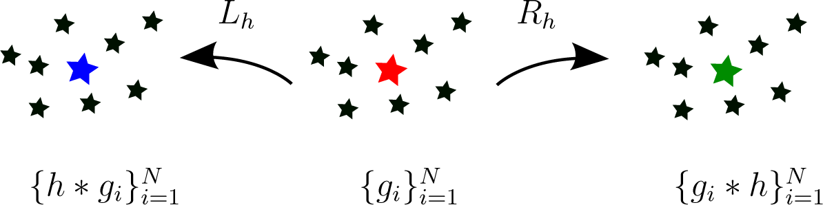
In fact, the definition of the mean on a Lie group should be consistent with the group structure. This consistency leads to several requirements of the mean, or properties. First, the mean of Lie group elements should be in the Lie group. Then, it seems natural to require that a left or right translation of the dataset should translate its mean accordingly. Figure 1 illustrates the case when this condition is fulfilled. Finally, the inversion of all data elements should lead to an inverted mean. A mean verifying all of these properties is said to be bi-invariant.

A naturally bi-invariant candidate for the mean on Lie groups is the group exponential barycenter [2] defined as follows. A group exponential barycenter m of the dataset {g_i}_i=1, …,_N is a solution, if there are some, of the following group barycenter equation:

$${\displaystyle \sum _{i=1}^N\text{Log}\left(m^{(-1)}*g_i\right)}=0$$

(1)

where Log is the group logarithm. As the group exponential barycenter is naturally bi-invariant, we call a group exponential barycenter a bi-invariant mean. The local existence and uniqueness of the bi-invariant mean have been proven if the dispersion of the data is small enough. “Local” means that the data are assumed to be in a sufficiently small normal convex neighborhood of some point of the Lie group.

Now, we want to provide a computational framework for the bi-invariant mean that would set the foundations for computations on Lie groups statistics in general. For that, we are interested in characterizing the global domains of existence and uniqueness of the bi-invariant mean. By “global domain”, we mean, for example, a ball of maximal radius, such that any probability measure with support included in it would have a unique bi-invariant mean. Note that there is a priori no problem having several means, which can be called several “modes”, or no mean at all. Our aim is rather to characterize the different situations that may occur: no mean, one unique mean, several means.

1.3. Using Riemannian and Pseudo-Riemannian Structures for Statistics on Lie Groups

To this aim, we are interested in additional geometric structures on Lie groups that could help, by providing computational tools. For example, we are interested in a distance on a Lie group, that could enable one to measure the radii of balls. Such a distance could obviously help with characterizing balls of maximal radius.

However, a Lie group is a group that carries an additional manifold structure, and one can define a pseudo-metric on a manifold, making it a pseudo-Riemannian manifold. Thus, we can add a pseudo-metric on Lie groups, which then induces a pseudo-distance. Could this additional pseudo-Riemannian structure help to define the statistical framework on Lie groups in practice?

We consider first the case of the Riemannian structure, i.e., when the pseudo-metric is in fact a metric (positive definite). Several definitions of the mean on Riemannian manifolds have been proposed in the literature: the Fréchet mean, the Karcher mean or the Riemannian exponential barycenter [3–8]. For example, the Riemannian exponential barycenters are defined as the critical points of the variance of the data, defined as: ${\sigma }^2(y)=\frac{1}{N}{\displaystyle {\sum }_{i=1}^N\mathrm{dist}{(x_i,y)}^2}$, where ${\left\{x_i\right\}}_{i=1}^N$ are the data and dist the distance induced by the Riemannian metric. The Riemannian framework provides theorems for the global existence and uniqueness domains of this mean [7–11], ensuring the computability of statistics on Riemannian manifolds. These represent exactly the kind of results that we would like to have for the bi-invariant mean on Lie groups. Thus, one may wonder if we can apply this computational framework for statistics on Lie groups and, more particularly, for the bi-invariant mean, by adding a Riemannian metric on the Lie group.

In fact, the notions of Riemannian mean and group exponential barycenter (or bi-invariant mean) coincide when the Riemannian metric is itself bi-invariant. In this case, the Riemannian geodesics coincide with the geodesics of the Cartan–Schouten connection [12]. Thus, we can use the computational framework for Riemannian means only if we can add a bi-invariant metric on a Lie group.

However, it is known that a Lie group does not have any bi-invariant Riemannian metric in general. The Lie group ST (n) of scalings and translations of ${\mathbb{R}}^n$, the Heisenberg group H, the Lie group UT (n) of upper triangular matrices of size n × n and the Lie group SE(n) of rotations and translations of ${\mathbb{R}}^n$ do not have any bi-invariant metric, while they admit a locally unique bi-invariant mean [2]. Therefore, if we want to characterize the bi-invariant mean with an additional geometric structure on Lie groups, we have to consider a structure that is more general than the Riemannian one.

The pseudo-Riemannian framework is a generalization of the Riemannian framework. Thus, it represents a tempting alternative for the characterization of the bi-invariant mean and for the definition of computational statistics on Lie groups in general. The pseudo-metric is not required to be positive definite anymore, only definite: the class of Lie groups that admit a bi-invariant pseudo-metric is larger than the class of those with a bi-invariant metric. Therefore, we could try to generalize the Riemannian statistical framework to a pseudo-Riemannian statistical framework and apply it for Lie groups. For instance, the mean on a pseudo-Riemannian manifold could still be defined as a critical point of the variance ${\sigma }^2(y)=\frac{1}{N}{\displaystyle {\sum }_{i=1}^N\mathrm{dist}{(x_i,y)}^2}$, but dist would now be the pseudo-distance induced by the pseudo-metric. Of course, existence and uniqueness theorems would have to be re-established, but we could get intuition from the Riemannian case.

In order to use the pseudo-Riemannian framework to characterize the bi-invariant mean, the first issue is: how many Lie groups do admit a bi-invariant pseudo-metric? Is it the case for the real Lie groups ST (n), H, UT (n) and SE(n), which have a locally unique bi-invariant mean?

1.4. Lie Groups and Lie Algebras with Bi-Invariant Pseudo-Metrics

If $\mathcal{G}$ is a connected Lie group, it admits a bi-invariant non-degenerate symmetric bilinear form if and only if its Lie algebra admits a nondegenerate symmetric bilinear inner product, also called a bi-invariant pseudo-metric. Lie algebras with bi-invariant pseudo-metric were known to exist since the 1910s with the classification of simple Lie algebra [13] and the well-known Cartan–Killing form, which is not degenerate in this case, but their specific study began in the 1950s with the works of [14,15]. Later, [16] started to study the properties of these Lie algebras from their structural point of view and introduced the decomposability orindecomposability of these Lie algebras as a direct sum of ideals. However, the decomposition of [16] was not enough to characterize all Lie algebras with bi-invariant pseudo-metrics, as some authors [17–19] remark that the so-called oscillator algebra arising in quantum mechanics carried a bi-invariant pseudo-metric without being decomposable in the sense of [16]. This leads, Medina and Revoy [20,21] and Keith [17] to build independently a classification of these Lie algebras, by showing that they all arise through direct sums and a structure, called the double extension in [20,21] and the bi-extension in [17].

These results have been complemented by [22] and then generalized by Bordemann to any non-associative algebras with the bi-invariant form through the T ^*-extension structure [23]. They have been completely described for certain dimensions in specific cases. The classification of the nilpotent quadratic Lie algebras of dimensions ≤ 7 is obtained in [24], of the real solvable quadratic Lie algebras of dimensions ≤ 6 in [25] and the irreducible non-solvable Lie algebras of dimensions ≤ 13 in [26]. The specific cases of indecomposable quadratic Lie algebras with pseudo-metrics of different indices have been studied: bi-invariant pseudo-metrics of index one are described in [21,27], of index two in [28] and finally of the general index in [29]. The dimension of the space of bi-invariant pseudo-metrics has been studied in [30] where bounds are provided.

Authors from other fields than pure algebra have also contributed to the study of bi-invariant pseudo-metrics. For example in functional analysis, Manin triples are a special type of Lie algebra with the bi-invariant pseudo-metric that allow one to interpret the solutions of the classical Yang–Baxter equation [31]. In this context, the Manin triples have been themselves classified for semi-simple Lie algebras in [32] and for complex reductive Lie algebra in [33].

Simultaneously, people started to gain interest in computational aspects on finite dimensional Lie algebras, implementing the identification of a Lie algebra from its structure constants given in any basis [34,35] or the Levi decomposition [36,37]. The state-of-the-art regarding implementations on finite dimensional Lie algebra is summarized in [38]. However, computations deal with the algebraic aspects of Lie algebras and, to the knowledge of the authors, do not consider metrics or pseudo-metrics.

1.5. Contributions and Outline

Our contribution is an algorithmic reformulation of a classification theorem for Lie algebras [20,21] that answers these questions. More precisely, taking a Lie group $\mathcal{G}$ as input, the algorithm constructs a bi-invariant pseudo-metric on $\mathcal{G}$ in the case of existence. Using this algorithm, we show that most Lie groups that have a locally unique bi-invariant mean do not possess a bi-invariant pseudo-metric. We conclude that, for the purpose of statistics on general real Lie groups and, more precisely, for the computational framework of the bi-invariant mean, generalizing the Riemannian statistical framework to a pseudo-Riemannian framework may not be the optimal program.

The paper is organized as follows. In the first section, we introduce notions on quadratic Lie groups that will be useful for the understanding of the paper. In the second section, we present the (tree-structured) algorithm that constructs bi-invariant pseudo-metrics on a given Lie group, in the case of existence. In the third section, we apply the algorithm on ST (n), H, UT (n) and SE(n) and show that most of them do not have any bi-invariant pseudo-metric.

2. Introduction to Lie Groups with Bi-Invariant Pseudo-Metrics

Here, we define the algebraic and geometric notions that will be used throughout the paper.

2.1. Quadratic Lie Groups and Lie Algebras

In the following, we consider finite dimensionalsimply connected Lie groups over the field $\mathbb{F}$, where $\mathbb{F}$ is $\mathbb{R}$ or $\mathbb{C}$.

2.1.1. Lie Groups

A Lie Group $\mathcal{G}$ is a smooth manifold with a compatible group structure. It is provided with an identity element e, a smooth composition law * : $\left(g,h\right)\mapsto g*h\in \mathcal{G}$ and a smooth inversion law Inv : $f\mapsto f^{\left(-1\right)}\in \mathcal{G}$. Its tangent space at g is written $T_g\mathcal{G}$.

The map $L_h:\mathcal{G}∍g\mapsto h*g\in \mathcal{G}$ is the left translation by hand is a diffeomorphism of $\mathcal{G}$. Therefore, its differential (at g), $D{L}_h(g):T_g\mathcal{G}\mapsto T_{L_{hg}}\mathcal{G}$ is an isomorphism that connects tangent spaces of $\mathcal{G}$. Similarly, one can define $R_h:\mathcal{G}∍g\mapsto g*h\in \mathcal{G}$, the right translation by h.

A vector field X on $\mathcal{G}$ is left invariant if (dL_h)(X(g)) = X(L_h(g)) = X(h * g) for each g, $h\in \mathcal{G}$. Similarly, one could define right invariant vector fields. The left invariant vector fields form a vector space that we denote $\mathrm{\Gamma }{(T\mathcal{G})}^L$ and that is isomorphic to $T_e\mathcal{G}$. The Lie bracket of two left invariant vector fields is a left-invariant vector field [39].

2.1.2. Lie Algebras

As $\mathrm{\Gamma }{(T\mathcal{G})}^L$ is closed under the Lie bracket of vector fields, we can look at $T_e\mathcal{G}$ as a Lie algebra. More precisely, we define $\mathfrak{g}$ the Lie algebra of $\mathcal{G}$ as $T_e\mathcal{G}$ with the Lie bracket induced by its identification with $\mathrm{\Gamma }{(T\mathcal{G})}^L$. The Lie algebra essentially captures the local structure of the group. In the case of Lie algebras of matrices, the Lie bracket corresponds to the commutator. For a more complete presentation of Lie groups and Lie algebras, we refer the reader to [40].

Writing the expression of the Lie bracket [,]_g on a given basis ${\mathcal{B}}_{\mathfrak{g}}={\left\{e_i\right\}}_{i=1}^n$ of $\mathfrak{g}$, we define the structure constants f_ijk as:

$${[e_i,e_j]}_{\mathfrak{g}}=f_{ijk}{e}_k$$

(2)

The structure constants f_ijk depend on the basis ${\mathcal{B}}_{\mathfrak{g}}$ chosen. They are always skew-symmetric in the first two indices, but they may have additional symmetry properties if we write them in a well-chosen basis (see below). The structure constants f_ijk completely determine the algebraic structure of the Lie algebra. Therefore, the structure constants are often the starting point, or the input, of algorithms on Lie algebras [34–36,38]. It will also be the case for the algorithm we present in this paper.

2.1.3. Pseudo-Metrics

A pseudo-metric <, > on $\mathcal{G}$ is defined as a smooth collection of definite inner products <, > |_g on each tangent space $T_g\mathcal{G}$. Then, $\mathcal{G}$ becomes a pseudo-Riemannian manifold. A metric is defined as a pseudo-metric whose inner products are all positive definite. In this case, $\mathcal{G}$ is called a Riemannian manifold.

The signature (p, q) of a pseudo-metric is the number (counted with multiplicity) of positive and negative eigenvalues of the real symmetric matrix representing the inner product <, > |_g at a point g and with respect to a basis of $T_g\mathcal{G}$. The signature is independent of the choice of the point g and on the basis at $T_g\mathcal{G}$. By definition, a pseudo-metric is definite; thus, there are no null eigenvalues, and we have p + q = n, where n is the dimension of $\mathcal{G}$. By definition, a metric is positive definite, and thus, its signature is (n, 0). Again, further details about such differential geometry can be found in [39].

2.1.4. Quadratic Lie Groups and Algebras

A left-invariant pseudo-metric is a pseudo-metric <, >, such that for all X, $Y\in T_g\mathcal{G}$ and for all g, $h\in \mathcal{G}$, we have:

$$\langle D{L}_h(g)X,D{L}_h(g)Y\rangle >{|{}_{L_{hg}}=\langle X,Y\rangle |}_g$$

(3)

where L_h is the left translation by h. In other words, the left translations are isometries for this pseudo-metric. Similarly, we can define right-invariant and bi-invariant pseudo-metrics <, >. Note that any Lie group admits a left (or right) invariant pseudo-metric: we can define an inner product on the Lie algebra $\mathfrak{g}=T_e\mathcal{G}$ and propagate it on each tangent space $T_g\mathcal{G}$ through DL_g(e) (or DR_g(e)). However, no Lie group admits a bi-invariant pseudo-metric.

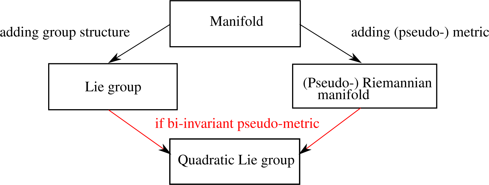
The Lie groups that admit a bi-invariant pseudo-metric are called quadratic Lie groups. The corresponding Lie algebras are called quadratic Lie algebras. Note that quadratic Lie groups or algebras are called differently in the literature. We find the appellation metrizable or metrized in [14–16], metric in [28,29], quasi-classical in [25] and, finally, quadratic in [24,26].

Figure 2 shows a summary of the structures that we just introduced.

We now recall that a non-degenerate bi-invariant inner product on a finite dimensional Lie algebra $\mathfrak{g}$ gives rise to a bi-invariant pseudo-metric on every Lie group whose Lie algebra is $\mathfrak{g}$ (see, for example, [41]). Therefore, we focus on Lie algebras from now on. We will still use the terms “pseudo-metric” or “metric” and the notation “<, >” in order to refer to the corresponding inner products on the Lie algebra $\mathfrak{g}=T_e\mathcal{G}$.

2.1.5. Characterization of Quadratic Lie Algebras

We give here different formulations of an equation characterizing a pair $(\mathfrak{g},<,>)$ as a quadratic Lie algebra. A Lie algebra $\mathfrak{g}$ is quadratic if and only if it has a pseudo-metric <, > verifying:

$${\forall }_{x,y,}t\in \mathfrak{g},<{[x,y]}_{\mathfrak{g}},t>+<y,{[x,t]}_{\mathfrak{g}}>=0$$

(4)

A proof for this characterization is given in [39] and [12].

First, taking advantage of the linearity in x, y, t, we can rewrite Equation (4) on basis vectors. Let ${\mathcal{B}}_{\mathfrak{g}}={\left\{e_i\right\}}_{i=1}^n$ be a basis of g; we consider: x = e_i, y = e_j and z = e_k. Thus, we can express the Lie bracket in terms of the structure constants, and we get:

$$\forall i,j,k\in \{1,\mathrm{..},n\}{f}_{ijl}<e_l,e_k>+f_{jkl}<e_l,e_j>=0$$

(5)

In particular, we observe that the structure constants written in a basis orthonormal with respect to a bi-invariant metric are totally skew-symmetric. The structure constants written in a basis orthonormal with respect to a bi-invariant pseudo-metric will have additional symmetric properties, as well.

Then, as we consider finite dimensional Lie groups, we can also rewrite Equation (4) in terms of matrices:

$$\forall x\in \mathfrak{g},A{(x)}^T.Z+Z.A(x)=0$$

(6)

where A(x) is the matrix of the endomorphism denoted [x, •], defined as $y\mapsto \left[x,y\right]$, and Z a symmetric invertible (not necessarily positive) matrix representing <, > on ${\mathcal{B}}_g$, the basis of $\mathfrak{g}$. Note that: $x\mapsto A(x)$ is itself linear.

Finally, taking advantage of the linearity again and writing: A(e_i) = A_i, we can again reformulate Equation (4), and we get:

$$\forall i\in \{1,\mathrm{..},n\},A_i^T.Z+Z.A_i=0$$

(7)

which is now a linear system of n matrix equations. Note that Equation (5) corresponds to Equations (7) written in coordinates.

2.1.6. How to Compute Bi-Invariant Pseudo-Metrics?

Given a Lie algebra $\mathfrak{g}$ as input, we see now that the computation of bi-invariant pseudo-metrics on $\mathfrak{g}$ amounts to the resolution of the linear system of Equations (7) for Z. The solutions of the linear system Equations (7) form a vector space, which is called the quadratic space $\mathcal{Q}(\mathfrak{g})$ [30]:

$$Q(\mathfrak{g})=\{Z\in \mathrm{Sym}(n)|\forall i\in \{1,\mathrm{..},n\},A_i^T.Z+Z.A_i=0\}$$

(8)

Obviously, the vector space $\mathcal{Q}(\mathfrak{g})$ contains invertible and non-invertible solutions. Recalling the definition of a pseudo-metric, we emphasize that we will be interested in invertible solutions only.

In order to solve the system of Equations (7) for Z, i.e., to compute the quadratic space $\mathcal{Q}(\mathfrak{g})$, we could adopt an analytic point of view. At i fixed, a single equation of the system of Equations (7) is a particular case of a Lyapunov equation that is studied in the context of control theory [42]. Thus, computational methods exist for studying one of our linear matrix equations [43]. For our purpose, however, we want to understand the structure of a quadratic Lie group, in order to get an intuition for the generalization to infinite dimensional Lie groups of diffeomorphisms. Thus, we do not rely on an analytic point of view to solve the system of Equations (7).

We rather consider the whole system of Equations (7) from an algebraic point of view. The pure algebraic point of view enables one to solve the system of Equations (7) completely in most cases, like in the examples provided at the end of the paper. In the other cases, it leads to a smaller system of equations that can be solved analytically or computationally. Thus, the algebraic point of view provides not only a theoretical understanding of quadratic Lie groups, it also either solves the problem or reduces the problem in order for the analytic point of view to solve it.

Therefore, we present in the next subsection the algebraic and geometric notions needed to set up, and later implement, the algebraic point of view.

2.2. Lie Algebra Representations

How can we understand the structure of a Lie algebra? An idea is to represent the Lie algebra elements as matrices acting on vectors. Then, the study of the behavior of these matrices helps to understand the Lie algebra as a whole. This is the purpose of the theory of Lie algebra representations, which we present briefly relying on [13,21,38,40] in all of this subsection.

2.2.1. Lie Algebras Representations

A $\mathfrak{g}$-representation on the vector space V is a Lie algebra homomorphism $\eta :\mathfrak{g}\mapsto \mathrm{gl}(V)$, which represents the elements of $\mathfrak{g}$ as matrices acting on the vector space V. The $\mathfrak{g}$-representations θ₁ and θ₂ are said to be isomorphic if there is an isomorphism of representations between them, i.e., an isomorphism of vector spaces $l:V_1\mapsto V_2$ that verifies: θ₂(x) ◦ l = l ◦ θ₁(x). We denote ${\mathrm{Hom}}_{\mathfrak{g}}\left(V_1,V_2\right)$ the vector space of isomorphisms of representations between V₁ and V₂.

In order to understand the representations of a Lie algebra $\mathfrak{g}$ and, thus, the Lie algebra $\mathfrak{g}$ itself, a strategy is to decompose the representations into smaller bricks, and then study those bricks. In this context, a $\mathfrak{g}$-subrepresentation of the $\mathfrak{g}$-representation V is a subspace of V stable by the elements of $\eta (\mathfrak{g})$. An irreducible $\mathfrak{g}$-subrepresentation is a $\mathfrak{g}$-subrepresentation without proper $\mathfrak{g}$-subrepresentation. An indecomposable $\mathfrak{g}$-subrepresentation is a $\mathfrak{g}$-subrepresentation that cannot be decomposed into $\mathfrak{g}$-subrepresentations.

Note that irreducibility implies indecomposability, but the converse is false: a $\mathfrak{g}$-subrepresentation can have a $\mathfrak{g}$-subrepresentation that does not have a supplementary that is also a $\mathfrak{g}$-subrepresentation (it would be “only” a vector space). Thus, it is not always possible to decompose a $\mathfrak{g}$-subrepresentation into irreducible $\mathfrak{g}$-subrepresentation, but only into indecomposable ones. In this context, a $\mathfrak{g}$-subrepresentation that can be decomposed into irreducible $\mathfrak{g}$-subrepresentations is called completely reducible.

2.2.2. Adjoint and Co-adjoint Representation

We can choose the vector space V on which we represent $\mathfrak{g}$. Taking $V=\mathfrak{g}$, thus representing the Lie algebra on itself, we define the so-called adjoint representation of $\mathfrak{g}$, $\mathrm{ad}:\mathfrak{g}∍x\mapsto \mathrm{ad}(x)={[x,•]}_{\mathfrak{g}}\in \mathfrak{g}\mathfrak{l}(\mathfrak{g})$. In its matricial version, we recognize the matrices A of the previous subsection. We see also that the set of matrices A_i defining the adjoint representation is equivalent to the set of structure constants of $\mathfrak{g}$.

We can rewrite again the Equation (4), but now in terms of the adjoint representation. We get:

$${\forall }_{x,y}t\in \mathfrak{g},<\mathrm{ad}(x).y,t>+<y,\mathrm{ad}(x).t>=0$$

(9)

Thus, the statement that $\mathfrak{g}$ is quadratic with bi-invariant pseudo-metric <, > is equivalent to the requirement that all endomorphisms ad(x) are skew-symmetric endomorphisms with respect to <, >. Recalling the matrix version of Equation (4), that is Equation (6), we see that solving for a bi-invariant Z amounts to finding a symmetric isomorphism of representations Z between the adjoint representation of $\mathfrak{g}$, written in its matricial form as $x\mapsto A(x)$ and the representation written in its matricial form as $x\mapsto -A{(x)}^T$.

If we choose to represent the Lie algebra $\mathfrak{g}$ on the dual vector space $\mathfrak{g}*$, i.e., we choose $V=\mathfrak{g}*$, we can define the co-adjoint representation $\theta :\mathfrak{g}∍x\mapsto \theta (x)ϵ\mathrm{gl}(\mathfrak{g}*)$, where < θ(x).f, t >=< f, ad(x).t > for f ∈ g*, x, y ∈ $\mathfrak{g}$ and <, > the inner product used to define the dual basis. If we write A(x) the matrix of the endomorphism ad(x), T (x) the matrix of the endomorphism θ(x) and Z the inner product defining the dual basis, the previous definition states that Z is in fact an isomorphism of representation between the co-adjoint representation $x\mapsto T(x)$ and the representation: $x\mapsto A{(x)}^T$.

Now, if the inner product <, > used to define the dual basis is bi-invariant, by identifying the vector spaces $\mathfrak{g}$ and $\mathfrak{g}*$, we can again rewrite Equation (4) to get:

$${\forall }_{x,y}t\in \mathfrak{g},<\mathrm{ad}(x).y,t>+<\theta (x).y,t>=0$$

(10)

We conclude that the bi-invariance of the inner product implies the following relation between the adjoint and co-adjoint representations: ad = −θ. As Z (that represents <, >) is an isomorphism of representations between the co-adjoint and the representation $x\mapsto A{(x)}^T$, we recover that the statement of Z being a bi-invariant pseudo-metric on $\mathfrak{g}$ is equivalent to Z being a symmetric isomorphism of representations between $x\mapsto A{(x)}^T$ and $x\mapsto -A{(x)}^T$.

2.2.3. Some Vocabulary of Algebra

The adjoint representation is related to the structure constants of $\mathfrak{g}$ and, thus, completely characterizes $\mathfrak{g}$. Thus, it links the language of abstract algebras and the language of representations for $\mathfrak{g}$.

For the special case of the adjoint representation ad, $\mathfrak{g}$-subrepresentations are ideals of $\mathfrak{g}$, irreducible $\mathfrak{g}$ -representations are minimal ideals of $\mathfrak{g}$ and indecomposable $\mathfrak{g}$ -representations are ideals of $\mathfrak{g}$ that cannot be decomposed into a direct sum of ideals of $\mathfrak{g}$. We will use the two languages of ideals or of representations.

If the adjoint representation is itself irreducible, but not one-dimensional, $\mathfrak{g}$ is said to be simple. If the adjoint representation is completely reducible, $\mathfrak{g}$ is said to be reductive. If the adjoint representation is completely reducible without one-dimensional subrepresentations, $\mathfrak{g}$ is semi-simple. If the adjoint representation is completely reducible with only one-dimensional subrepresentations, $\mathfrak{g}$ is abelian. A reductive Lie algebra is thus the sum (in the sense of subrepresentations) of a semi-simple Lie algebra and an abelian Lie algebra.

2.2.4. Some Vocabulary of Geometry

An ideal I of a Lie algebra B is said to be isotropic with respect to a pseudo-metric given on B if I ∩ I^⊥ ≠ {0}. The ideal I is said to be totally isotropic if I ⊂ I^⊥. The intersection between I and I^⊥ represents the vectors that are orthogonal to themselves and, thus, that have zero norm, even if they are themselves non-zero.

Thus, isotropic ideals appear only in the case of a pseudo-metric that is not a metric. From the intuition provided by theoretical physics, we can interpret the vectors in I ∩ I^⊥ as photons: they have zero mass even if they have non-zero velocity.

2.3. Constructions with Lie Algebra Representations

We have seen that we can study the structure of a given Lie algebra by looking at its representations and more particularly at its adjoint representation. Here, we study decompositions of the adjoint representation that will be pertinent for the characterization of quadratic Lie algebras: the direct sum decomposition and the double extension decomposition. We show how these decompositions can be implemented in a computational framework. In this subsection, we use the notation (B, [,]_B) to denote the Lie algebra, because this is the notation that we will use in the core of our algorithm (see Section 4).

2.3.1. Definition of Direct Sum

B = B₁ ⊕_B B₂ is the direct sum of B₁, B₂ if:

• B = B₁ ⊕ B₂ in terms of vector spaces,
• [B, B₁]_B ⊂ B₁ and [B, B₂]_B ⊂ B₂, making B₁ and B₂ subrepresentations of the adjoint representation of B, in other words: ideals of B.

This decomposition was first studied by [16]. We illustrate it with the matrices A representing the adjoint representation $b\mapsto {[b,•]}_B$ of B, i.e., the matrices denoted: $b\mapsto A(b)={[b,•]}_B$. The direct sum of B is equivalent to the decomposition of the adjoint representation into the B-representations B₁ and B₂ i.e.,:

$$A(b)=\left(\begin{array}{cc}A(b_1)& 0\\ 0& A(b_2)\end{array}\right)$$

(11)

on a basis respecting B = B₁ ⊕_B B₂. Note that we write ⊕_B to emphasize the fact that this direct sum decomposition is more than the direct sum decomposition into vector spaces.

2.3.2. Direct Sum Decomposition and Bi-Invariant Pseudo-Metrics

We have the following property: B being quadratic is equivalent to B₁ and B₂ being quadratic. Indeed, if <, >_B1, <, >_B2 are bi-invariant pseudo-metrics on B₁, B₂ and represented by the matrices $Z_{B_1}$, $Z_{B_2}$, then:

$$Z_{B_1{\oplus }_B{B}_2}=\left(\begin{array}{cc}{Z}_{B_1}& 0\\ 0& Z_{B_2}\end{array}\right)$$

(12)

is bi-invariant on B. Conversely, if <, >_B is bi-invariant on B, its restrictions <, >_B |_B1 and <, >_B |_B2 are bi-invariant on B₁, B₂ [20,21].

2.3.3. Computing the Direct Sum

The direct sum decomposition of a Lie algebra B into indecomposable subrepresentations is unique, up to isomorphisms. In practice, writing ${\mathcal{B}}_B={\left\{e_k\right\}}_{k=1}^{\dim (B)}$ a basis of B and A_k = A(e_k), computing the direct sum decomposition of B into indecomposable B_i’s amounts to the simultaneous bloc diagonalization of the matrices A_k.

2.3.4. Definition of Double Extension

B = W ⊕ S ⊕ S* is the double extension of W by a simple S if:

• B = W ⊕ S ⊕ S^* in terms of vector spaces,
• (W, [, ]_W) is a Lie algebra and [S, W ]_B ⊂ W makes W a S-representation,
• (S, [, ]_S) is a simple Lie subalgebra of B: [s, s′]_B = [s, s′]_S,
• S* is the dual space of S and [S, S*]_B ⊂ S* makes S* the co-adjoint representation,
• ∀w, w′ ∈ W : [w, w′]_B = [w, w′]_W + β(w, w′) where β : Λ²W ↦S* is a (skew-symmetric)

S-equivariant map, i.e., a map that commutes with the action of S.

This definition relies on the framework introduced in [21], or in [17] under the appellation “bi-extension”. Here, we can illustrate it with the matrices representing the adjoint representation b ↦[b, •]_B of B, i.e., the matrices denoted: b ↦A(b). The double extension decomposition is equivalent to the following decomposition of the adjoint representation of B:

$$A(b)=\left(\begin{array}{ccc}{[w,•]}_W+{[s,•]}_B& {[w,•]}_B& 0\\ 0& {[s,•]}_S& 0\\ \beta (w,•)& {[f,•]}_B& {[s,•]}_B\end{array}\right)$$

(13)

on a basis respecting B = W ⊕ S ⊕ S* and b = w + s + f. Note that, in the blocks of the matrix A(b), we have identified endomorphisms with their corresponding matrices.

The definition of double extension uses a number of different notations. First, we recognize ad(s) = [s, •]_S and ad(w) = [w, •]_W to be respectively the adjoint representation of S (on S) and the adjoint representation of W (on W ). However, [s, •]_B is a S-representation on W that has nothing to do with the adjoint (the adjoint is a representation of a Lie algebra on itself).

Then, we should be careful with the structures that are manipulated. For example, we can consider the vector space S* as an abelian Lie subalgebra of B. However, we cannot consider W as a subalgebra of B. The skew-symmetric map β represents precisely the corresponding obstruction.

2.3.5. Double Extension Decomposition and Bi-Invariant Pseudo-Metrics

We have the following property: B being quadratic is equivalent to W being quadratic. Indeed, if <, >_W is bi-invariant on W, represented by Z_W, then:

$$Z_{W\oplus S\oplus S*}=\left(\begin{array}{ccc}{Z}_W& 0& 0\\ 0& 0& \mathbb{I}\\ 0& \mathbb{I}& 0\end{array}\right)$$

(14)

is bi-invariant on B. Conversely, if B is quadratic and written as a double extension of W with S simple (or one-dimensional), then the restriction <, >_W =<, >_B |_W is bi-invariant [20,21]. Note here that we can write the II-blocks, because the basis of S and S^* are chosen to be duals of each other. If two different basis were chosen, the corresponding bi-invariant pseudo-metric on B = W ⊕ S ⊕ S^* would have the form:

$$Z_{W\oplus S\oplus S*}=\left(\begin{array}{ccc}{Z}_W& 0& 0\\ 0& 0& L\\ 0& L^T& 0\end{array}\right)$$

(15)

with L an invertible matrix representing precisely the change of basis. More precisely, by computing Equation (6) on this last Z_W⊕S⊕S* while choosing s ∈ S, we show that L is necessarily an isomorphism of S-representations on S and I, i.e., L ∈ Hom_S(S, S*). This remark will be used in practice in the algorithm (see Section 4).

2.3.6. Computing Double Extensions

Contrary to the direct sum decomposition, the decomposition of a quadratic Lie algebra B as a double extension is not necessary unique. For example, given a quadratic indecomposable non-simple B, we can build a double extension decomposition from each minimal ideal of B [21]. It proceeds as follows. We take a minimal ideal I of B and consider I^⊥ its orthogonal with respect to a bi-invariant pseudo-metric <, >_B. The decomposition:

$$B=W\oplus S\oplus S^{*}\text{where}:W=I^{\perp }/I,S=B/I^{\perp }\text{and}{S}^{*}=I$$

is a double extension of W with S simple (or one-dimensional). Moreover, one can show that I and I^⊥ verify the following properties:

• I is abelian,
• I^⊥ is a maximal ideal,
• I ⊂ I^⊥ (total isotropy),
• [I, I^⊥] = 0 (commutativity),
• codim(I^⊥) = dim(I).

These necessary conditions are taken from [16,20,21].

In practice, in our algorithm, we will have to build a double extension from a B in order to compute a bi-invariant pseudo-metric on B, if it exists (see Section 4). Therefore, even if we know an abelian minimal ideal I of B, we will not have its orthogonal I^⊥ needed for the construction shown above: we do not know any bi-invariant pseudo-metric, as we want to build one!Thus, given an abelian minimal ideal I, we shall test all ideals J that could be an I^⊥ for a bi-invariant pseudo-metric, i.e., all ideals J that verify the necessary conditions listed above.

We show here that the only plausible ideals that can play the role of I^⊥ are either J = C_B(I) the centralizer of I in B in the case C_B(I) ≠ B or the maximal ideals of codimension one containing I in the case C_B(I) = B.

We have seen above that the first necessary condition for a J to be an I^⊥ is its commutativity with I: [I, J] = 0. We recall that the centralizer C_B(I) of I in B is defined as the set of elements that commute with I. Thus: J ⊂ C_B(I).

Another necessary condition for a plausible J is to be a maximal ideal. As I is an ideal, C_B(I) is also an ideal. Thus, J is a maximal ideal included in the ideal C_B(I): we have necessarily J = C_B(I) in the case C_B(I) ≠ B. In this case, the condition I ⊂ J is fulfilled as I is abelian. The last necessary condition to check is codim(C_B(I)) = dim(I).

However, if C_B(I) = B, then we shall look for maximal ideals of B. However, in this case, I commutes with all elements of B, and therefore, I is necessarily of dimension one as a minimal ideal. Therefore, we shall look for maximal ideals J of codimension one. Adding the last necessary condition, we conclude that in the case C_B(I) = B, we shall consider only maximal ideals of codimension one containing I.

3. Structure of Quadratic Lie Groups

Here, we characterize the structure of quadratic Lie algebras, using the constructions defined in the previous section. We first present a reformulation of a classification theorem of quadratic Lie algebras. Then, we emphasize which Lie algebras we add by asking for a bi-invariant pseudo-metric instead of a bi-invariant metric. We finally investigate how we can go from a bi-invariant pseudo-metric to a bi-invariant dual metric on a special class of Lie algebra with bi-invariant pseudo-metrics.

3.1. A Classification Theorem

To characterize the structure of a quadratic Lie algebra, we use a reformulation of a classification theorem than can be found in [21] or [17].

Theorem 1 (Classification of quadratic Lie algebras). The Lie algebra$\mathfrak{g}$ is quadratic if and only if its adjoint representation decomposes into indecomposable subrepresentations B that are of the following types:

• Type (1): B is simple (or one-dimensional),
• Type (2): B = W ⊕ S ⊕ S* is a double extension of a quadratic W by S simple (or one-dimensional).

This means that any quadratic Lie algebra writes $g=B_1{\oplus }_{\mathfrak{g}\cdots }{\oplus }_{\mathfrak{g}}{B}_N$, where each B is of Type (1) or of Type (2). In particular, we can already conclude that any reductive (a fortiori, semi-simple or abelian) Lie algebra $\mathfrak{g}$ is quadratic. Moreover, if $\mathfrak{g}$ is quadratic, but not reductive, then $\mathfrak{g}$ has non-irreducible indecomposable subrepresentations, and these are necessarily double extensions of Type (2).

We recall that the notions of representation decomposition come from a simultaneous diagonalization of matrices. Therefore, they depend on the base field $\mathbb{F}$: a Lie algebra reductive in $\mathbb{R}$ is reductive in $\mathbb{C}$, but the converse is false. Thus, being quadratic also depends on the field that we consider. A Lie algebra quadratic on $\mathbb{R}$ will be quadratic on $\mathbb{C}$, but the converse is false.

3.1.1. Elementary Bi-Invariant Pseudo-Metrics

The previous characterization of quadratic Lie algebras in terms of their structure is useful in practice. It enables one to construct a type of bi-invariant pseudo-metric <, ${>}_{\mathfrak{g}}$ that exists necessarily on a quadratic $\mathfrak{g}$. We call this type of pseudo-metrics the elementary bi-invariant pseudo-metrics of $\mathfrak{g}$.

The elementary bi-invariant pseudo-metric <, >_B of a one-dimensional Lie algebra B is defined to be the multiplication. The elementary bi-invariant pseudo-metric <, >_B of a simple Lie algebra B is defined to be the Killing form. Now, let us define recursively the elementary bi-invariant pseudo-metrics of a general quadratic $\mathfrak{g}$.

Let us be given a quadratic Lie algebra $\mathfrak{g}$ on which we know an auxiliary bi-invariant pseudo-metric <, ${>}_{\mathfrak{g}}$ (not necessarily of the elementary type). First, we decompose the adjoint representation of $\mathfrak{g}$ into indecomposable subrepresentations $\mathfrak{g}=B_1{}_{{\oplus }_{\mathfrak{g}\cdots }{\oplus }_{\mathfrak{g}}}{B}_N$. Then, we study separately the two cases: the B’s of Type (1) and the B’s of Type (2).

On the B’s of Type (1), we define the elementary bi-invariant pseudo-metric <, >_B as above: the multiplication if B is one-dimensional or the Killing form if B is simple.

On the B’s of Type (2), we build a double extension. To this aim, we consider a minimal ideal I, and using the auxiliary bi-invariant pseudo-metric <, ${>}_{\mathfrak{g}}$ of g, we compute I^⊥. We get the double extension B = W ⊕ S ⊕ S^* with W = I^⊥/I, S = B/I^⊥ and S* = I. We construct an elementary bi-invariant pseudo-metric <, >_W on W recursively. We then define an elementary bi-invariant pseudo-metric <, >_B on the double extension B = W ⊕ S ⊕ S* to be of the form of Equation (14).

Finally, we define the elementary bi-invariant pseudo-metric <, ${>}_{\mathfrak{g}}$ on the direct sum decomposition $\mathfrak{g}=B_1{}_{{\oplus }_{\mathfrak{g}\cdots }{\oplus }_{\mathfrak{g}}}{B}_N$ to be of the form of Equation (12). This construction defines (and proves the existence of) elementary bi-invariant pseudo-metrics on a quadratic $\mathfrak{g}$.

3.2. Riemannian and Pseudo-Riemannian Quadratic Lie Groups

The previous characterization of quadratic Lie algebras can be refined to distinguish between quadratic Lie algebras that admit bi-invariant metrics with respect to quadratic Lie algebras with bi-invariant pseudo-metrics. In other words, it answers the questions: which Lie algebras do we add by removing the positivity of the metric?

3.2.1. Studying the Signature

We recall from Section 2 that a metric on $\mathfrak{g}$ of dimension n has signature (n, 0). Now, we take a quadratic $\mathfrak{g}$ that is decomposed into indecomposable pieces $\mathfrak{g}=B_1{}_{{\oplus }_{\mathfrak{g}\cdots }{\oplus }_{\mathfrak{g}}}{B}_N$, where the B_i are either simple (or one-dimensional) or double extensions. The signature on the direct sum is the sum of the signatures on the B_i [39]:

$${\mathrm{sgn}}_{\mathfrak{g}}={\mathrm{sgn}}_B{}_{{}_1}+\dots +{\mathrm{sgn}}_{B_N}$$

(16)

Therefore, asking for a positive definite signature on $\mathfrak{g}$ is equivalent to asking for a positive definite signature on each of the B’s.

If B is simple, it possesses a bi-invariant metric if and only if it is compact. If B is a double extension, a bi-invariant pseudo-metric has necessary a non-positive definite signature of the form [21]:

$${\mathrm{sgn}}_B={\mathrm{sgn}}_W+\left(m,m\right)$$

(17)

where m is the dimension of the minimal ideal I used to build the double extension.

We conclude that $\mathfrak{g}$ admits a bi-invariant metric if and only if its indecomposable parts are simple compact or one-dimensional, i.e., if and only if $\mathfrak{g}$ is reductive with compact simple parts.

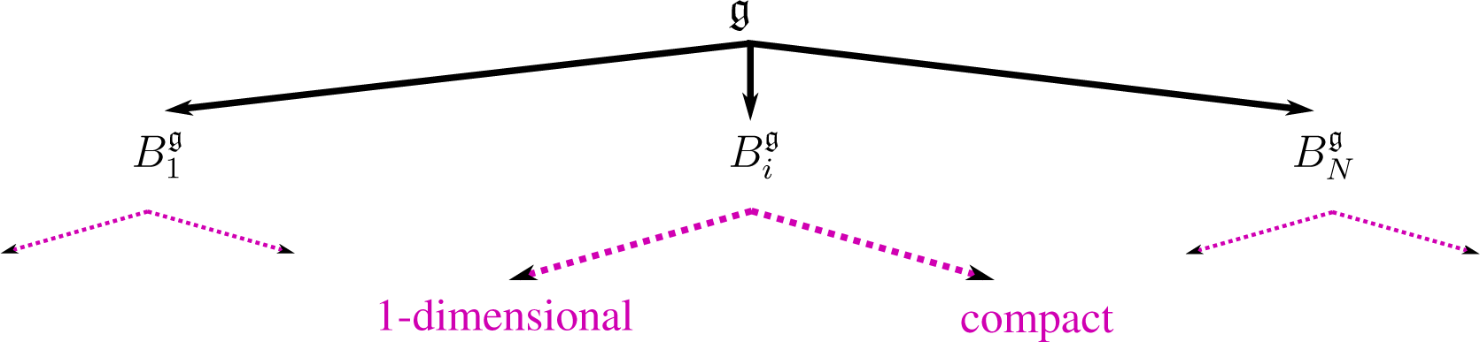
3.2.2. Comparison

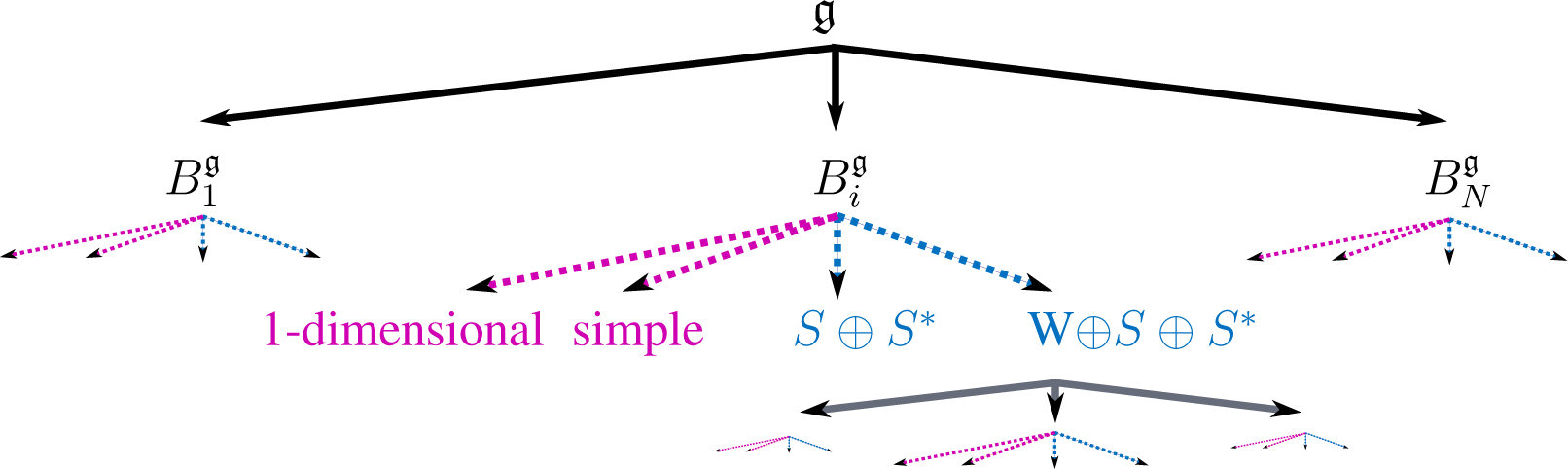
The trees of Figures 3 and 4 illustrate the comparison between Lie algebras with bi-invariant metrics and Lie algebras with bi-invariant pseudo-metrics.

Thus, going from Riemannian to pseudo-Riemannian enables to add the simple algebras that generalize the compact algebras and the double extension structures (in blue) with its recursive construction that is not present in the Riemannian case.

3.3. From a Bi-Invariant Pseudo-Metric to a Bi-Invariant Dual Metric?

We investigate here a special case of Lie algebras that we gain by going from Riemannian to pseudo-Riemannian: the double extension of W = {0} by a compact simple Lie algebra K, which is an example of a Manin triple (see [31,32]). We will see in this subsection that we can view this case as a Riemannian case by changing the base field $\mathbb{F}$ (which is $\mathbb{R}$ or $\mathbb{C}$ for us) to its dual algebra $\mathbb{D}$. This development is a new contribution, which is a justification and an extension of the dual quaternions for SE(3).

3.3.1. Dual Numbers and Vectors

Given a field $\mathbb{F}$, the algebra $\mathbb{D}$ of dual numbers over this field is defined as $\mathbb{D}=\mathbb{F}+ϵ\mathbb{F}$, where ϵ² = 0 and ϵ ≠ 0 defines the multiplication [44]. We can define an m-dimensional dual vector space ${\mathbb{D}}^m={\mathbb{F}}^m+ϵ{\mathbb{F}}^m$, whose elements are dual vectors. Note here that the term “vector” is abusive in the sense that a vector space is usually defined on a field, not on an algebra. In the following, in order to study the properties of the dual vector space, we will use the dual map:

$$\begin{array}{l}\psi :{\mathbb{F}}^m\oplus {\mathbb{F}}^m\mapsto {\mathbb{D}}^m\\ x_0+x_{ϵ}\mapsto x_0+ϵx_{ϵ}\end{array}$$

using the same notation ψ for mapping either to dual numbers or to dual vectors.

3.3.2. From the Double Extension $\mathfrak{g}=K\oplus K*$ to Its Dual $\overline{\mathfrak{g}}=K+ϵK*$

Now, we consider the double extension $\mathfrak{g}$ = K ⊕ K*, where K is compact simple and dim(K) = m, so that $\dim (\mathfrak{g})=2m$. We take the following elementary bi-invariant pseudo-metric on $\mathfrak{g}$:

$$Z_{K\oplus K*}=\left(\begin{array}{cc}\mathbb{I}& \mathbb{I}\\ \mathbb{I}& 0\end{array}\right)$$

(18)

As K and K* have same $\mathbb{F}$-dimension m, we consider the dual space $\overline{\mathfrak{g}}=K+ϵK*$, of $\mathbb{D}$-dimension m. Its dual vectors write $\overline{x}=x_0+ϵ.x_{\in }$, where x₀ ∈ K and x_ϵ ∈ K*.

Proposition 1. The dual map:

$$\begin{array}{l}\psi :\mathfrak{g}=K\oplus K*\mapsto \overline{\mathfrak{g}}\\ x_0+x_{ϵ}\mapsto x_0+ϵx_{ϵ}\end{array}$$

is an isomorphism of Lie algebras that respects the sum K ⊕ K*. The canonical inner product on$\mathfrak{g}$ is bi-invariant and corresponds to the bi-invariant pseudo-metric Z_K⊕K* above.

This can been shown as follows. First, consider the Lie bracket on $\overline{\mathfrak{g}}$ inherited from ψ. We have:

$$\begin{array}{l}[\psi (x),\psi (x^{\prime })]=[x_0+ϵx_{\in },{x^{\prime }}_0+ϵ{x^{\prime }}_{\in }]\\ =[x_0,{x^{\prime }}_0]+ϵ([x_0,{x^{\prime }}_{\in }]+[x_{\in },{x^{\prime }}_0])(\text{as}{\in }^2=0)\\ =\psi ([x,x^{\prime }])(\text{definition of double extension})\end{array}$$

which proves the isomorphism of Lie algebras.

We now show that the pseudo-metric Z_K⊕K* on the Lie $\mathbb{F}$-algebra $\mathfrak{g}$ maps to the canonical metric $Z=\mathbb{I}$ on the Lie $\mathbb{D}$-algebra $\overline{\mathfrak{g}}$:

$$\begin{array}{l}\psi {(x)}^T.\psi (x^{\prime })={(x_0+ϵ.x_{\in })}^T.({x^{\prime }}_0+ϵ{x^{\prime }}_{\in })\\ =x_0^T.{x^{\prime }}_0+ϵ(x_{\in }^T.{x^{\prime }}_0+x_0^T.{x^{\prime }}_{\in })\\ =\psi (x^T.Z_{K\oplus K*.x})(\text{using}\psi \text{for dual number})\end{array}$$

In others words, the spaces $\mathfrak{g}$ and $\overline{\mathfrak{g}}$ are isometric. However, again, the term “isometric” is abusive, as we recall that $\mathfrak{g}$ and $\overline{\mathfrak{g}}$ are not defined on the same field, the latter being defined on an algebra.

3.3.3. Towards Statistics on Dual Riemannian Manifolds

We have shown that a double extension $\mathfrak{g}=K\oplus K*$ of W = {0} by a compact simple K, endowed with a bi-invariant pseudo-metric, is isometrically isomorphic to a dual Lie algebra $\mathfrak{g}$ with a bi-invariant metric. Thus, we could think of generalizing the theory of statistics on Riemannian manifolds to a theory of statistics on dual Riemannian manifolds. However, the fact that the space is defined on an algebra may cause some problems.

3.3.4. Generalization?

One could wonder if we can use this construction for any general double extension. However, we should note that this construction takes advantage of the fact that K* is totally isotropic and abelian. The element ϵ, such that ϵ² = 0, enables one to represent the commutativity of K* (Lie bracket is null) and the self-orthogonality of K* (the inner product is null) at the same time. A general Lie algebra with the bi-invariant pseudo-metric is not necessarily decomposable into two subspaces of same dimension, such that one of them is abelian and isotropic. For example, take a Lie algebra of an odd dimension.

4. An Algorithm to Compute Bi-Invariant Pseudo-Metrics on a Given Lie Group

We go back to the general case of any quadratic Lie algebra over the field $\mathbb{F}\left(\mathbb{F}=\mathbb{R}\text{or}\mathbb{C}\right)$. We present in this section an algorithm that computes bi-invariant pseudo-metrics on a Lie algebra given as input.

Then, we show how one could generalize the algorithm to compute all bi-invariant pseudo-metrics on $\mathfrak{g}$. Finally, we apply the algorithm to some Lie groups known to possess a unique bi-invariant mean: we find that most of them are not quadratic.

4.1. The Algorithm: Computation of One Bi-Invariant Pseudo-Metric

For the computations, we will use matrix representations Z of pseudo-metrics <, >, where the basis will be specified. The input is ${\mathcal{B}}_{\mathfrak{g}}={\left\{e_i\right\}}_{i=1}^n$, a basis of $\mathfrak{g}$ and the structure constants f_ijk on this basis. The output is a symmetric invertible matrix $Z_{\mathfrak{g}}$ on the basis ${\mathfrak{B}}_{\mathfrak{g}}$, representing an elementary bi-invariant pseudo-metric, or a message of error: “the Lie algebra $\mathfrak{g}$ is not quadratic”.

4.1.1. Core of the Algorithm

The core of the algorithm tests the structure of the Lie algebra given as input, to determine if it matches the characteristic tree-structure of quadratic Lie algebras described in the Section 3 (see Figure 4). Simultaneously with the progress through the tree, the algorithm tries to construct recursively an elementary bi-invariant pseudo-metric <, ${>}_{\mathfrak{g}}$ by testing all possible candidates. If it succeeds, we return the bi-invariant elementary pseudo-metric, proving that $\mathfrak{g}$ is quadratic. If not, we conclude that $\mathfrak{g}$ is not quadratic, and we return the error message. More precisely, the algorithm is divided into four steps as follows.

Step 1, direct sum decomposition: In this step, we decompose the adjoint representation of $\mathfrak{g}$ into indecomposable B’s, in other words: we decompose $\mathfrak{g}$ as a direct sum of B’s.

$$\mathfrak{g}=B_1{\oplus }_{\mathfrak{g}}\dots {\oplus }_{\mathfrak{g}}{B}_N$$

(19)

An implementation of this step can be found in [35].

From now on, we work on the basis ${{\mathcal{B}}^{\prime }}_{\mathfrak{g}}$ that respects the direct sum: $\mathfrak{g}=B_1{\oplus }_{\mathfrak{g}}\dots {\oplus }_{\mathfrak{g}}{B}_N$. The B’s are indecomposable Lie algebras; thus, we can take advantage of the classification theorem 1 of Section 3. In the following two steps, we test if each B is either of Type (1) (one-dimensional or simple) or of Type (2) (a double extension). testing Type (1): In this step, we test if the indecomposable B is of Type (1), i.e., if B is one-dimensional or simple (see the dichotomy of Theorem 1).

To test if B is one-dimensional, we can obviously count the number of basis vectors of B in the basis ${{\mathcal{B}}^{\prime }}_{\mathfrak{g}}$. If B is found one-dimensional, we return the multiplication, which is an elementary bi-invariant pseudo-metric on B.

To test if B is simple, we use a function that computes the radical of the Levi decomposition of B [45]. The indecomposable piece B is simple if and only if the radical is null. Such a function can be found in [36]. If B is found simple, we return the Killing form, which is an elementary bi-invariant pseudo-metric.

If B is neither one-dimensional nor simple, we conclude that B is not of Type (1). We test in the following step if B is of Type (2).

Step 3, testing Type (2): In this step, we test if B is of Type (2), i.e., if B is a double extension of a quadratic W by a simple S (see the dichotomy of Theorem 1). We recall that the double extension structure of B is not necessarily unique. Therefore, it might seem that we need to test all possible candidates for a double extension structure of B, in order to answer if B is of Type (2). We proceed slightly differently.

As B is indecomposable and not of Type (1) (see the previous steps), B being of Type (2) is equivalent to B being quadratic. More precisely, at this step of the algorithm, the following assertions are equivalents:

• B is of Type (2),
• B is quadratic,
• ∀I minimal, I abelian, there is a double extension decomposition of B,
• ∃I minimal, abelian, such that there is a double extension decomposition of B.

Thus, we will consider only one minimal ideal I of B and try to construct a double extension out of it, of the form: B = W ⊕ S ⊕ I. Note that this step will need to call the algorithm recursively, to determine if the candidate for W in the double extension structure is quadratic or not. The details of this step are below.

Step 3.a: First, we compute a minimal ideal I. More precisely, recalling the necessary conditions of the double extension structure of Section 2, we compute I, an abelian minimal ideal, which is also a minimal abelian ideal. A function that finds a minimal abelian ideal of B can be derived from an algorithm of [46] that computes all abelian ideals of B: we can choose one of minimal dimension among those.

Step 3.b: Then, we compute C_B(I), the maximal ideals J’s and the corresponding candidates for the double extension structure of B. The computation of C_B(I) is implemented in [47].

If C_B(I) ≠ B, we take J = C_B(I) and verify the condition codim(J) = dim(I). If the condition is not fulfilled, there is no double extension structure possible for B. Therefore, we conclude that B is not of Type (2).

If C_B(I) = B, we compute the maximal ideals J of B of codimension one containing I (see Section 2). If no such ideals are found, there is no double extension structure possible for B. Again, in this case, we conclude that B is not of Type (2).

If J’s are found, we compute the corresponding double extension candidates of B, one per J, as:

$$B=W\oplus S\oplus S*\text{where:}W=J/I,S=B/J\text{and}:S*=I.$$

(20)

We call the algorithm recursively on W, i.e., we determine recursively if W is quadratic. If there is no double extension candidate with a quadratic W, we conclude that B is not of Type (2). Otherwise, we keep the double extension candidates that have a quadratic W (with an elementary bi-invariant pseudo-metric Z_W ).

Step 3.c: Then, we try to compute an elementary pseudo-metric for all double extension candidates of the form: B = W ⊕ S ⊕ S*, where W = J/I is quadratic with corresponding Z_W, S = B/J and S* = I. Given a double extension candidate, we know from Section 2 that an elementary pseudo-metric on B has the form:

$$Z_{B=W\oplus S\oplus I}=\left(\begin{array}{ccc}{Z}_W& 0& 0\\ 0& 0& L\\ 0& L^T& 0\end{array}\right)$$

(21)

where L ∈ Hom_S(S, I).

Therefore, we need to compute Hom_S(S, I). We recall that S is simple; thus, its adjoint representation is irreducible. As we are in the case of a finite dimensional irreducible representation, we can apply Schur’s lemma. Its general form states that Hom_S(S, S) is an associative division algebra over $\mathbb{F}\left(=\mathbb{R}or\mathbb{C}\right)$, which is of finite degree, because S is finite dimensional [48]. When the base field is $\mathbb{F}=\mathbb{C}$, we use the fact that a finite-dimensional division algebra over an algebraically closed field is necessarily itself. Thus, ${\mathrm{Hom}}_S\left(S,S\right)=\mathbb{C}$ and ${\dim }_{\mathbb{C}}\left({\mathrm{Hom}}_S\left(S,S\right)\right)=1$. When the base field is $\mathbb{F}=\mathbb{R}$, we use the Frobenius theorem, which asserts that the only real associative division algebras are $\mathbb{R}$, $\mathbb{C}$ or $\mathrm{H}$, the field of quaternionnumbers [49]. Thus, Hom_S(S, S) is $\mathbb{R}$, $\mathbb{C}$ or $\mathrm{H}$, and dim_R(Hom_S(S, S)) is 1, 2 or 4. Now, if I and S are isomorphic, Hom_S(S, I) is isomorphic to Hom_S(S, S) and, thus, of maximal dimension four over $\mathbb{F}$. Otherwise, if I and S are not isomorphic, we have Hom_S(S, I) = {0}.

The computation of Hom_S(S, I) is implemented in [50], more generally for any finite-dimensional modules of a finitely generated algebra.

Step 3.d: To conclude Step 3, we determine if one of the possible elementary pseudo-metrics computed above is bi-invariant. To this aim, we plug the expression of Z_B=W⊕S⊕I into Equations (7) and solve it for L. Thus, the initial system of Equations (7) has been reduced to an equation in maximum one (complex case) or in four (real case) parameters.

We run this step for each double extension candidate. If a bi-invariant elementary pseudo-metric Z_B is found on one of the candidates, we return Z_B. Otherwise, we conclude that B is not of Type (2).

Step 4, construction of a bi-invariant pseudo-metric on the whole $\mathfrak{g}$: In this step, we construct a bi-invariant (elementary) pseudo-metric on $\mathfrak{g}$, if it exists. If one B of the direct sum decomposition $\mathfrak{g}=B_1{\oplus }_{\mathfrak{g}}\dots {\oplus }_{\mathfrak{g}}{B}_N$ is neither of Type (1), nor of Type (2), we conclude from Theorem 1 that $\mathfrak{g}$ is not quadratic. We return the error message. Otherwise, we glue together the elementary bi-invariant pseudo-metrics Z_B’s that have been returned on the B’s.

More precisely, we follow the construction of Section 2 to build the elementary bi-invariant pseudo-metric ${Z^{\prime }}_{\mathfrak{g}}$ on the basis ${{\mathcal{B}}^{\prime }}_{\mathfrak{g}}$ of $\mathfrak{g}$ that respects the direct sum decomposition:

$$Z_{\mathfrak{g}=B_{1\oplus \mathfrak{g}\dots \oplus \mathfrak{g}{B}_N}}=\left(\begin{array}{ccc}{Z}_{B_1}& 0& 0\\ 0& \ddots & 0\\ 0& 0& Z_{B_N}\end{array}\right)$$

(22)

Finally, we perform a change of basis from ${{\mathcal{B}}^{\prime }}_{\mathfrak{g}}$ to ${\mathcal{B}}_{\mathfrak{g}}$ in order to return $Z_{\mathfrak{g}}$, an elementary bi-invariant pseudo-metric on the basis of the Lie algebra given as input.

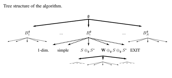
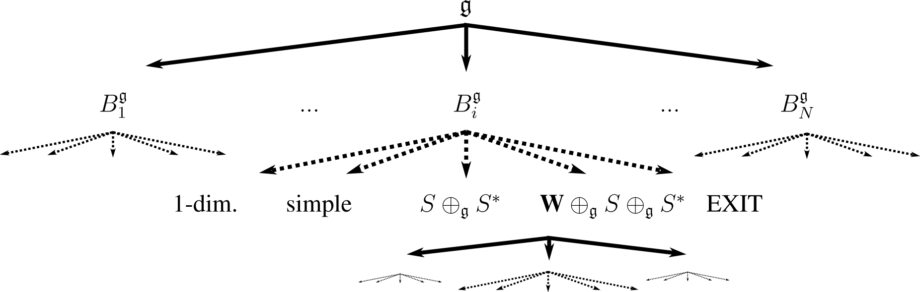
4.1.2. Tree Structure of the Algorithm

The algorithm has a natural tree structure presented in Figure 5. The bi-invariant pseudo-metric $Z_{\mathfrak{g}}$ is computed in a postfix manner. A tree level corresponds to a reduction of an adjoint representation: reduction of $\mathfrak{g}$ into B’s for the first level, reductions of the W ’s into B’s for the others. The arrows in dashes represent the cases that we investigate to test if $\mathfrak{g}$ is quadratic. If B is not in one of such cases, then B is not quadratic, so neither is $\mathfrak{g}$, and we exit the algorithm.

In pseudo-code, the algorithm is written as follows.

Algorithm 1. Computation of a bi-invariant pseudo-metric on $\mathfrak{g}$.

Algorithm 1. Computation of a bi-invariant pseudo-metric on $\mathfrak{g}$.

This gives a bi-invariant pseudo-metric on the Lie algebra $\mathfrak{g}$. We can then make it a bi-invariant pseudo-metric on the Lie group $\mathcal{G}$ by propagating it through DL_g(e) (or DR_g(e)) on all tangent spaces $T_{\mathfrak{g}}\mathcal{G}$ (see Section 2).

All in all, the algorithm allows one to compute one bi-invariant pseudo-metric of $\mathfrak{g}$, i.e., one invertible element of the quadratic space $\mathcal{Q}(\mathfrak{g})$. We can generalize the algorithm, in order to compute all bi-invariant pseudo-metrics of $\mathfrak{g}$, thus the whole quadratic space $\mathcal{Q}(\mathfrak{g})$. This is the purpose of the next subsection.

4.2. Generalization of the Algorithm: Computation of All Bi-Invariant Pseudo-Metrics

Here, we present how one should proceed in order to compute all bi-invariant pseudo-metrics of a given Lie algebra $\mathfrak{g}$, i.e., the whole quadratic space $\mathcal{Q}(\mathfrak{g})$. Note that the dimension of $\mathcal{Q}(\mathfrak{g})$ is unknown in the general case [30]. However, the algorithmic procedure allows one to compute the space anyway.

We follow the strategy of the previous algorithm: we decompose $\mathfrak{g}$ into indecomposable B’s; we compute the quadratic spaces $\mathcal{Q}(B)$ for each of them and then glue these spaces together to get $\mathcal{Q}(\mathfrak{g})$.

4.2.1. Computing the Quadratic Space of Indecomposable Lie Algebras

In this step, we compute the quadratic space for all indecomposable pieces B’s of $\mathfrak{g}$, the simple (or one-dimensional) and the double extensions.

The quadratic space of a one-dimensional piece B is the weighted multiplication, so the whole base field $\mathbb{F}$:

$$\mathcal{Q}\left(B\right)=\{Z_B=\alpha \mathbb{I}|\forall \alpha ϵ\mathbb{F}\}=\mathbb{F}$$

(23)

The quadratic space of a simple piece B is the vector space spanned by the Killing form.

$$Q(B)=\{Z_B=\alpha Z_{\text{killing}}|\forall \alpha ϵ\mathbb{F}\}$$

(24)

The quadratic space of a double extension B = W ⊕ S ⊕ S*, where the basis of S and S* are chosen duals, is given by:

$$\mathcal{Q}(B)=\left\{Z_B=\left(\begin{array}{ccc}{Z}_W& M& N\\ M^T& \alpha Z_{Killing}& \beta \mathbb{I}\\ N^T& \beta \mathbb{I}& (0)\end{array}\right)|\begin{array}{c}\forall \alpha ,\beta ϵ\mathbb{F},\forall Z_W\in \mathcal{Q}(W),\\ \forall M,N\text{solutions of equations derived from}\left(7\right)\end{array}\right\}$$

(25)

We leave to the reader the computations of the equations derived from Equations (7) that M and N are solving. Because of the dimension reduction, these equations can be solved in a lot of interesting cases. In our computations on selected Lie groups in the next subsection, N and N are vectors or scalars, for example.

4.2.2. Computing the Quadratic Space of a Direct Sum

The second step is the computation of the quadratic space of a direct sum $\mathfrak{g}=B_1{\oplus }_{\mathfrak{g}}\dots {\oplus }_{\mathfrak{g}}{B}_N$, given the quadratic spaces of each of its indecomposable pieces B_i. This gives:

$$\mathcal{Q}(\mathfrak{g})=\left\{Z_{\mathfrak{g}}\in \mathrm{sym}(n)|\text{s.t. for}i\in \{1,\mathrm{..}N\}(\text{block index}):\begin{array}{c}{Z}_{{\mathfrak{g}}_{ii}}=Z_{B_I}\in \mathcal{Q}(B_i)\\ Z_{{\mathfrak{g}}_{ij}}=M_{ij}\text{if}i<j\end{array}\text{if}i=j\right\}$$

(26)

where M_ij is a matrix that solves the following equation, derived from Equations (7):

$$A{(b_i)}^T.M_{ij}+M_{ij}.A(b_j)=0\forall b_i\in B_i,\forall b_j\in B_j$$

(27)

In summary, the problem of computing all bi-invariant pseudo-metrics of a given $\mathfrak{g}$ amounts to the resolution of a reduced number of algebraic equations of lower dimension.

4.3. Results of the Algorithm on Selected Lie Groups

We run our algorithm manually to determine if a bi-invariant pseudo-metric exists on some real Lie groups for which there is a locally unique bi-invariant mean: SE(n), ST (n), H and UT (n), for $n\in \mathbb{N}*$ [2].

We run the computations manually and illustrate them, for each example, with the corresponding progress through the tree of the algorithm. The results show that most of these Lie groups are not quadratic.

4.3.1. Scalings and Translations ST (n)

The Lie group ST (n) comprises uniform scalings together with translations of ${\mathbb{R}}^n$. It is the semi-direct product ${\mathbb{R}}_{+}^{*}\propto {\mathbb{R}}^n$, its elements being written (λ, t). More precisely, ST (n) is defined by its action on ${\mathbb{R}}^n:(\lambda ,t).x=\lambda .x+t$. The group law and the group inversion are written as follows: (λ₁, t₁) * (λ₂, t₂) = (λ₁.λ₂, λ₁ * t₂ + t₁) and (λ, t)⁽⁻¹⁾ = (1/λ, −t/λ).

The Lie algebra $\mathfrak{st}(n)$ comprises the $\left(\mu ,u\right)\in R\oplus {\mathbb{R}}^n$ with Lie bracket:

$$\left[\left({\mu }_1,u_1\right),\left({\mu }_2,u_2\right)\right]=\left(0,{\mu }_2.u_1-{\mu }_1.u_2\right).$$

(28)

Input: We choose the basis $(D,{\left\{P_a\right\}}_{a=1}^n)$ defined as: D = (1, 0) and P_a = (0, e_a) with ${(e_a)}_{a=1}^n$ the canonical basis of ${\mathbb{R}}^n$. In this basis, the structure constants can be read in the following Lie brackets:

$$\begin{array}{l}\left[P_a,P_b\right]=0,\hfill \\ \left[D,P_a\right]=P_a,\hfill \\ \left[D,D\right]=0.\hfill \end{array}$$

Step 1: From the expression of the Lie brackets above, we can compute all ideals of $\mathfrak{st}(n)$ manually and find: Span(P₁), …, Span(P_n) and their linear combinations. We remark that there is no ideal containing D. Thus, $\mathfrak{st}(n)$ cannot be written as the direct sum of ideals, i.e., $\mathfrak{st}(n)$ is indecomposable.

Step 2: First, as $n\in \mathbb{N}*$, we have $\text{dim (st}(n))>1$. Thus, $\mathfrak{st}(n)$ is not one-dimensional. Then, as Span(P₁), for example, is an ideal, $\mathfrak{st}(n)$ is not simple. We conclude that $\mathfrak{st}(n)$ is not of Type (1).

Step 3: We take I = Span(P₁), which is obviously a minimal abelian ideal. From the commutation relations given by the Lie brackets, we see that $C_{\mathfrak{st}(n)}(I)=Span({\left\{P_a\right\}}_{a=1}^n)$, and we are in the case $C_{\mathfrak{st}(n)}(I)\ne \mathfrak{st}(n)$. Thus, there is only one double extension candidate, with $J=C_{\mathfrak{st}(n)}(I)$. We define $S=\mathfrak{st}(n)/J=\text{Span}(D)$ and W = J/I = Span(P₂,..P_n). We call the algorithm recursively on W, which decomposes into one-dimensional ideals on which we return the multiplication.

The S-representation on S is the null representation: [D, D] = 0. The S-representation on I is the trivial representation: [D, P₁] = P₁. Hence, I and S are not isomorphic S-representations, and Hom_S(S, I) is zero. We conclude that $\mathfrak{st}(n)$ is not of Type (2).

Output: We have found that $\mathfrak{st}(n)$ is indecomposable and neither of Type (1) nor of Type (2). Thus, $\mathfrak{st}(n)$ is not quadratic: there is no bi-invariant pseudo-metric <, > on $\mathfrak{st}(n)$.

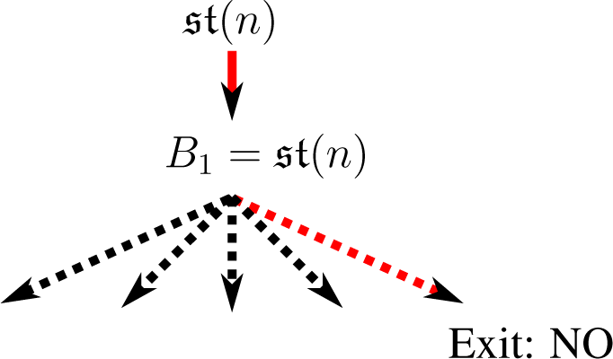
This reasoning is illustrated on Figure 6 through the tree representation of the algorithm.

4.3.2. Heisenberg Group H

The Heisenberg group H comprises 3D upper triangular matrices M of the form:

$$M=\left(\begin{array}{ccc}1& x& z\\ 0& 1& y\\ 0& 0& 1\end{array}\right).$$

Thus, an element of this group can be written as $(x,y,z)ϵ{\mathbb{R}}^3$, with corresponding group law (x₁, y₁, z₁) * (x₂, y₂, z₂) = (x₁ + x₂, y₁ + y₂, z₁ + z₂ + x₁ * y₂) and group inversion (x, y, z)⁽⁻¹⁾ = (−x, −y, −z + xy).

The Lie algebra $\mathfrak{h}$ comprises the nilpotent matrices:

$$N=\left(\begin{array}{ccc}0& p& c\\ 0& 0& q\\ 0& 0& 0\end{array}\right).$$

Input: A basis for $\mathfrak{h}$ is thus (P, Q, C) with clear notations. In this basis, the structure constants can be read in the following Lie brackets:

$$\begin{array}{l}[C,P]=0,\\ [C,Q]=0,\\ [P,Q]=C.\end{array}$$

Step 1: From the expression of the Lie brackets above, we can compute all ideals of $\mathfrak{h}$ manually, and we find: Span(C), Span(C, P) and Span(C, Q). We remark that there is no ideal whose supplementary is also an ideal. Thus, $\mathfrak{h}$ is indecomposable.

Step 2: $\mathfrak{h}$ is obviously not one-dimensional. Moreover, as Span(C), for example, is an ideal, $\mathfrak{h}$ is not simple. We conclude that $\mathfrak{h}$ is not of Type (1).

Step 3: We take I = Span(C), which is a minimal abelian ideal of $\mathfrak{h}$. From the commutation relations given by the Lie brackets, we compute the commutator of I, and we see that we are in the case $C_{\mathfrak{h}}(I)=\mathfrak{h}$. Thus, we consider all maximal ideals of h that are of codimension one and contain I. We get J = Span(C, P) or J = Span(C, Q); thus, we have two double extension candidates. By symmetry in P ↔ Q (see the structure constants), we can consider J = Span(C, P) only, without lost of generality. We define $S=\mathfrak{h}/J=\text{Span}\left(Q\right)$ and W = J/I = Span(P). We call the algorithm recursively on W. As W is one-dimensional, W is quadratic, and we return Z_W = 1.

The S-representation on S is given by the bracket [Q, Q] = 0: it is the null representation. The S-representation on I is given by the bracket [Q, C] = 0: it is also the null representation. The isomorphism of vector spaces L that maps C on Q is an isomorphism of representations, whose matricial form is the identity in our basis. The dimension of Hom_S(S, I) is obviously one.

Thus, we plug:

$$Z_{W\oplus S\oplus I}=\left(\begin{array}{ccc}1& 0& 0\\ 0& 0& 1\\ 0& 1& 0\end{array}\right)$$

into Equation (6) to determine if it is bi-invariant. Computations show that it is not. We conclude that $\mathfrak{h}$ is not of Type (2).

Output: We have found that $\mathfrak{h}$is indecomposable and neither of Type (1) nor of Type (2). Thus, $\mathfrak{h}$ is not quadratic: there is no bi-invariant pseudo-metric<,> on $\mathfrak{h}$.

We try the algorithm on the general Heisenberg algebra ${\mathfrak{h}}_{2m+1}$, which is defined abstractly by the basis $\left\{C,{\left\{P_i\right\}}_{i=1}^m,{\left\{Q_j\right\}}_{j=1}^m\right\}$ and the Lie bracket:

$$\begin{array}{c}\left[C,P_i\right]=0,\hfill \\ \left[C,Q_j\right]=0,\hfill \\ \left[P_i,Q_j\right]={\delta }_{ij}\hfill \end{array}$$

where δ is the Kronecker symbol. We are in the same situation as with $\mathfrak{h}$, except that W is abelian (but not necessarily one-dimensional). We thus decompose W into abelian one-dimensional ideals, and we return the following elementary bi-invariant pseudo-metric:

$$Z_W=\left(\begin{array}{ccc}1& 0& 0\\ 0& \ddots & 0\\ 0& 0& 1\end{array}\right).$$

However, we exit the algorithm as previously. Thus, the algorithm confirms that the general ${\mathfrak{h}}_{2m+1}$ has no bi-invariant pseudo-metric [20].

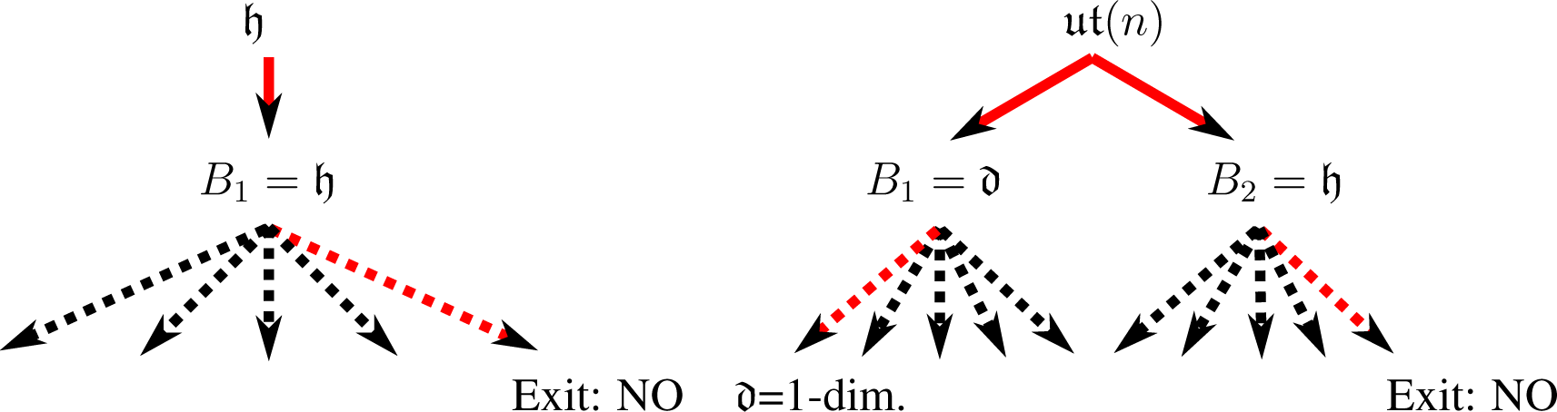
This reasoning is illustrated on the left hand side of Figure 7 through the tree representation of the algorithm.

4.3.3. The Group of Scaled Upper Unitriangular Matrices UT (n)

The group UT (n) comprises the upper triangular matrices M of the form: M = λ.Id + N, where λ > 0 and N an upper triangular nilpotent matrix.

The Lie algebra $\mathfrak{ut}\left(n\right)$ comprises the matrices of the form X = μ.Id + Y, where $\mu \in \mathbb{R}$ and Y an upper triangular nilpotent matrix, the Lie bracket being the commutator of matrices.

Now, $\mathfrak{ut}\left(n\right)$ is decomposable into the one-dimensional Lie algebra generated by II and the Heisenberg algebra $\mathfrak{h}$. As h has no bi-invariant pseudo-metric, neither does $\mathfrak{ut}\left(n\right)$.

This reasoning is illustrated on the right hand side of Figure 7 through the tree representation of the algorithm.

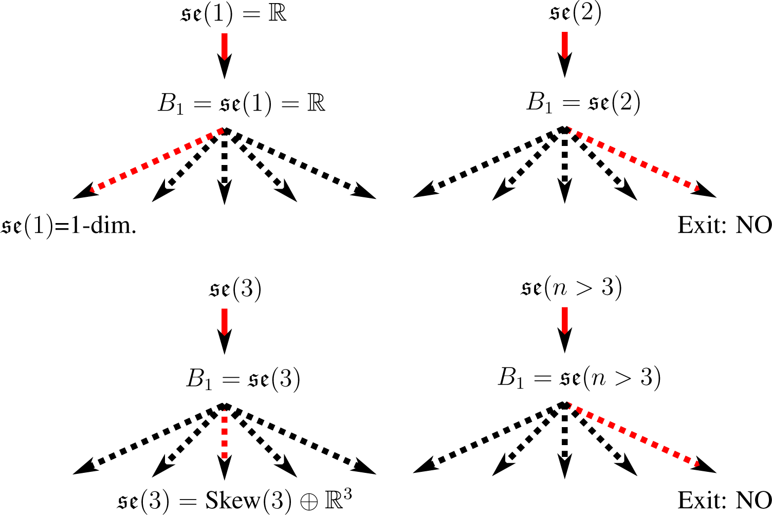
4.3.4. Rigid Body Transformations SE(n)

The group of isometries SE(n) comprises rotations together with translations of ${\mathbb{R}}^n$. It is the semi-direct product $SO(n)\propto {\mathbb{R}}^n$, its elements being written (R, t). More precisely, SE(n) is defined by its action on ${\mathbb{R}}^n$ as (R, t).x = R.x + t. The group law and the group inversion are (R₁, t₁) * (R₂, t₂) = (R₁.R₂, R₁ * t₂ + t₁) and (R, t)⁽⁻¹⁾ = (R⁽⁻¹⁾, R⁽⁻¹⁾.(−t)).

The Lie algebra $\mathfrak{se}$(n) comprises the $\left(A,u\right)\in Skew\left(n\right)\oplus {\mathbb{R}}^n$ with Lie bracket:

$$[(A_1,u_1),(A_2,u_2)]=(A_1{}_{.}{A}_2-A_{2.}{A}_1,A_1{}_{.}{u}_2-A_2{}_{.}{u}_1)$$

(29)

Input: We choose the basis: $({\left\{J_{ij}\right\}}_{1\le }{}_{i<j\le n},{\left\{Pa\right\}}_{a=1}^n)$ with $J_{ij}=e_{i.e.,}{}_j^T-e_j.e_i^T$ and ${\left\{P_a\right\}}_{a=1}^n$ the canonical basis of ${\mathbb{R}}^n$. In this basis, the structure constants can be read in the following Lie brackets:

$$\begin{array}{l}[J_{ij},J_{kl}]={\delta }_{ik}.J_{jl}-{\delta }_{jk}.J_{il}+{\delta }_{jl}.J_{ik}-{\delta }_{jl}.J_{jk},\\ [J_{ij},P_a]={\delta }_{aj}.P_i-{\delta }_{ai}.P_j,\\ [P_a,P_b]=0,\end{array}$$

with δ the Kronecker symbol.

As preliminaries, we show that $P=\text{Span}({\left\{P_a\right\}}_{a=1}^n)$ is the only proper ideal of $\mathfrak{se}$(n). First, we see from the Lie brackets that P is a proper ideal of $\mathfrak{se}$(n). Suppose that $\mathfrak{se}$(n) has another proper ideal K. Then, either K ∩ P is a proper ideal of $\mathfrak{se}$(n) included in P or K ⊂ $\mathfrak{so}$(n) is a proper ideal of $\mathfrak{se}$(n). P does not contain any proper ideal of $\mathfrak{se}$(n), because $\mathfrak{so}$(n) acts transitively on P with the Lie bracket. We can show that $\mathfrak{so}$(n) does not contain any proper ideal of $\mathfrak{se}$(n) (considering independently the case n = 4). Thus, P is the only proper ideal of $\mathfrak{se}$(n).

Step 1: The Lie algebra $\mathfrak{se}$(n) has only one ideal P. Thus, $\mathfrak{se}$(n) cannot be decomposed as a direct sum of ideals. We conclude that $\mathfrak{se}$(n) is indecomposable.

Step 2: If n = 1, $\mathfrak{se}$(1) is obviously one-dimensional. We return the multiplication, which is a bi-invariant pseudo-metric on $\mathfrak{se}$(1). Otherwise, dim(se(n)) > 1. As P is an ideal of $\mathfrak{se}$(n), $\mathfrak{se}$(n) is not simple. We conclude that $\mathfrak{se}$(1) is quadratic with the multiplication as the bi-invariant pseudo-metric and that $\mathfrak{se}$(n) with n > 1 is not of Type(1). We go on with n > 1.

Step 3: We take I = P and J = C_se(n)(I) = P = I. The necessary condition codim(J) = dim(I) is verified only for n = 3. We conclude that $\mathfrak{se}$(n) is not of Type (2) if n ≠ 3. We go on with n = 3. We compute S = $\mathfrak{se}$(3)/P ∼ $\mathfrak{so}$(3) and W = P/P = {0}.

In order to study the S-representations, we write the Lie bracket as:

$$\begin{array}{l}[J_m,J_n]={\in }_{mnp\cdot }{J}_p,\\ [J_m,P_a]={\in }_{map\cdot }{P}_p,\\ [P_a,P_b]=0.\end{array}$$

where we define J₁ = J₂₃, J₂ = J₃₁ and J₃ = J₁₂. The S-representation on S is the adjoint representation: [J_m, J_n] = _mnp.J_p. The S-representation on I = P is given by: [J_m, P_a] = _map.P_p. It is also the adjoint representation. The isomorphism of vector spaces L that maps each P_a on J_a is an isomorphism of representations whose matricial form is the identity in our basis.

Hence, we write Z_se(3) on the decomposition S ⊕ I = $\mathfrak{so}$(3) ⊕ P with basis $({\left\{J_a\right\}}_{a=1}^3,{\left\{P_a\right\}}_{a=1}^3)$ and get:

$$Z_{\mathfrak{se}(3)}=\left(\begin{array}{cc}0& {\mathbb{I}}_3\\ {\mathbb{I}}_3& 0\end{array}\right).$$

(30)

We plug it into Equations (7). Running the computation shows that the pseudo-metric Z_se(3) is bi-invariant on $\mathfrak{se}$(3). Z_se(3) is actually known as the Klein form [51].

Output: $\mathfrak{se}$(1) is quadratic; we return the multiplication, which is a bi-invariant pseudo-metric on $\mathfrak{se}$(1). $\mathfrak{se}$(3) is quadratic; we return the Klein form, which a bi-invariant pseudo-metric on $\mathfrak{se}$(3). Otherwise, $\mathfrak{se}$(n) is indecomposable and neither of Type (1) nor of Type (2): it is not quadratic.

This reasoning is illustrated on Figure 8 through the tree representation of the algorithm.

We can build the whole quadratic space of $\mathfrak{se}$(3). This gives the two-dimensional vector space:

$${\mathcal{Q}}_{(\mathfrak{se}(3))}=\left\{\left(\begin{array}{cc}\alpha Z_{\text{killing}}& \beta .\mathbb{I}\\ \beta .\mathbb{I}& 0\end{array}\right)|\forall \alpha ,\beta ϵ\mathbb{F}\right\}$$

(31)

Moreover, we have recognized in $\mathfrak{se}$(3) the special case of a double extension K ⊕ K* of W = {0} by a compact Lie algebra K = $\mathfrak{so}$(3). Therefore, the dual structure presented in Section 3 can be used in practice. We recall that we can represent the elements of SO(3) as unit quaternions. Thus, we can represent the elements of SE(3) as unit dual quaternions [52]. A generalization of the theory of Riemannian statistics to a theory of dual Riemannian statistics would thus be useful for rigid body transformations, which are present in many different fields.

5. Conclusions

In this paper, we have presented an algorithmic method to compute a bi-invariant pseudo-metric on a Lie group, in the case of existence. The method allows one to test simultaneously if the Lie group given as input is quadratic or not. We indicated how to compute all pf the bi-invariant pseudo-metrics on the given Lie group. First, the algorithm by itself represents a contribution to the field of computational Lie algebra.

Then, regarding statistics on Lie groups, which was our original motivation, we see two consequences of this article. First, it enables one to distinguish, from a practical point of view, Lie groups on which a future pseudo-Riemannian theory of statistics could be used and implemented. This is the case of SE(3), the Lie group of rotations and translations of the 3D space, which is found in various fields.

Second, this paper shows that a general Lie group with bi-invariant mean does not admit a bi-invariant metric. Therefore, if one wants to define a general theory of statistics that works for all Lie groups, one needs to find a geometric framework beyond the Riemannian and the pseudo-Riemannian ones.

References

- Thompson, D.W.; Bonner, J.T. On Growth and Form; Cambridge University Press: Cambridge, UK, 1992. [Google Scholar]
- Pennec, X.; Arsigny, V. Exponential Barycenters of the Canonical Cartan Connection and Invariant Means on Lie Groups. In Matrix Information Geometry; Springer: New York, NY, USA, 2012; pp. 123–168. [Google Scholar]
- Fréchet, M. L’intégrale abstraite d’une fonction abstraite d’une variable abstraite et son application a la moyenne d’un élément aléatoire de nature quelconque; La Revue Scientifique: Paris, France, 1944. [Google Scholar]
- Fréchet, M. Les éléments aléatoires de nature quelconque dans un espace distancié. Annales de l’institut Henri Poincaré 1948, 10, 215–310. [Google Scholar]
- Karcher, H. Riemannian center of mass and mollifier smoothing. Commun. Pure Appl. Math. 1977, 30, 509–541. [Google Scholar]
- Kendall, W.S. Probability, Convexity, and Harmonic Maps with Small Image I: Uniqueness and Fine Existence. Proc. Lond. Math. Soc. 1990, s3-61, 371–406. [Google Scholar]
- Émery, M.; Mokobodzki, G. Sur le barycenter d’une probabilité dans une variété. Séminaire de probabilités de Strasbourg 1991, 25, 220–233. [Google Scholar]
- Corcuera, J.M.; Kendall, W.S. Riemannian Barycentres and Geodesic Convexity. Math. Proc. Camb. Philos. Soc. 1998, 127, 253–269. [Google Scholar]
- Huiling, L. Estimation of Riemannian Barycentres. LMS J. Comput. Math. 2004, 7, 193–200. [Google Scholar]
- Yang, L. Riemannian median and its estimation. LMS J. Comput. Math. 2010, 13, 461–479. [Google Scholar]
- Afsari, B. Riemannian Lp center of mass: existence, uniqueness, and convexity. Proc. Am. Math. Soc. 2011, 139, 655–673. [Google Scholar]
- Sternberg, S. Lectures on Differential Geometry; Prentice-Hall Mathematics Series; Prentice-Hall: Englewood Cliffs, NJ, USA, 1964. [Google Scholar]
- Cartan, E. Sur la Structure des Groupes de Transformations Finis et Continus, 2nd ed.; Vuibert.: Paris, France, 1933; p. 157 S. [Google Scholar]
- Tsou, S.T.; Walker, A.G. XIX. Metrisable Lie Groups and Algebras. Proc. R. Soc. Edinb. Sect. A Math. Phys. Sci. 1957, 64, 290–304. [Google Scholar]
- Tsou, S.T. XI. On the Construction of Metrisable Lie Algebras. Proc. R. Soc. Edinb. Sect. A Math. Phys. Sci. 1962, 66, 116–127. [Google Scholar]
- Astrakhantsev, V.V. Decomposability of metrizable Lie algebras. Funct. Anal. Appl. 1978, 12, 210–212. [Google Scholar]
- Keith, V. On Invariant Bilinear Forms on Finite-dimensional Lie Algebras. Ph.D. Thesis, Tulane University, New Orleans, LA, USA, 1984. [Google Scholar]
- Medina, A.; Revoy, P. Les groupes oscillateurs et leurs reseaux. Manuscr. Math. 1985, 52, 81–95. [Google Scholar]
- Guts, A.K.; Levichev, A.V. On the Foundations of Relativity Theory. Doklady Akademii Nauk SSSR 1984, 277, 1299–1303. [Google Scholar]
- Medina, A. Groupes de Lie munis de pseudo-métriques de Riemann bi-invariantes. Sémin. géométrie différentielle 1981-1982, Montpellier 1982, Exp. 637 p. (1982) 1982. [Google Scholar]
- Medina, A.; Revoy, P. Algèbres de Lie et produit scalaire invariant. Annales scientifiques de l’École Normale Supérieure 1985, 18, 553–561. [Google Scholar]
- Hofmann, K.H.; Keith, V.S. Invariant quadratic forms on finite dimensional lie algebras. Bull. Aust. Math. Soc. 1986, 33, 21–36. [Google Scholar]
- Bordemann, M. Nondegenerate invariant bilinear forms on nonassociative algebras. Acta Mathematica Universitatis Comenianae 1997, 66, 151–201. [Google Scholar]
- Favre, G.; Santharoubane, L. Symmetric, invariant, non-degenerate bilinear form on a Lie algebra. J. Algebra 1987, 105, 451–464. [Google Scholar]
- Campoamor-Stursberg, R. Quasi-Classical Lie Algebras and their Contractions. Int. J. Theor. Phys. 2008, 47, 583–598. [Google Scholar]
- Benayadi, S.; Elduque, A. Classification of quadratic Lie algebras of low dimension. J. Math. Phys. 2014, 55, 081703. [Google Scholar]
- Hilgert, J.; Hofmann, K. Lorentzian cones in real Lie algebras. Monatsh. Math. 1985, 100, 183–210. [Google Scholar]
- Kath, I.; Olbrich, M. Metric Lie algebras with maximal isotropic centre. Math. Z. 2004, 246, 23–53. [Google Scholar]
- Kath, I.; Olbrich, M. Metric Lie algebras and quadratic extensions. Transform. Groups 2006, 11, 87–131. [Google Scholar]
- Duong, M.T. A New Invariant of Quadratic Lie Algebras and Quadratic Lie Superalgebras. Ph.D. Theses, Université de Bourgogne, Dijon, France, 2011. [Google Scholar]
- Drinfeld, V.G. Quantum Groups; American Mathematics Society: Providence, RI, USA, 1987; pp. 798–820. [Google Scholar]
- Belavin, A.; Drinfeld, V. Triangle Equations and Simple Lie Algebras. In Math. Phys. Rev.; Harwood Academic: Newark, NJ, USA, 1998; Volume 4. [Google Scholar]
- Delorme, P. Classification des triples de Manin pour les algebres de Lie reductives complexes: Avec un appendice de Guillaume Macey. J. Algebra 2001, 246, 97–174. [Google Scholar]
- Rand, D. {PASCAL} programs for identification of Lie algebras: Part 1. Radical—A program to calculate the radical and nil radical of parameter-free and parameter-dependent lie algebras. Comput. Phys. Commun. 1986, 41, 105–125. [Google Scholar]
- Rand, D.; Winternitz, P.; Zassenhaus, H. On the identification of a Lie algebra given by its structure constants. I. Direct decompositions, levi decompositions, and nilradicals. Linear Algebra Appl. 1988, 109, 197–246. [Google Scholar]
- Cohen, A.M.; Graaf, W.A.D.; Rónyai, L. Computations in finite-dimensional Lie algebras. Discret. Math. Theor. Comput. Sci. 1997, 1, 129–138. [Google Scholar]
- Ronyai, L.; Ivanyos, G.; Küronya, A.; de Graaf, W.A. Computing Levi Decompositions in Lie algebras. Appl. Algebra Eng. Commun. Comput. 1997, 8, 291–303. [Google Scholar]
- De Graaf, W. Lie Algebras: Theory and Algorithms; North-Holland Mathematical Library; Elsevier: Amsterdam, The Netherlands, 2000. [Google Scholar]
- Postnikov, M. Geometry VI: Riemannian Geometry; Encyclopaedia of Mathematical Sciences; Springer: New York, NY, USA, 2001. [Google Scholar]
- Bourbaki, N. Lie Groups and Lie Algebras; Springer: Paris, France, 1989; Chapters 1–3. [Google Scholar]
- Milnor, J. Curvatures of left invariant metrics on lie groups. Adv. Math. 1976, 21, 293–329. [Google Scholar]
- Bartels, R.H.; Stewart, G.W. Solution of the Matrix Equation AX + XB = C [F4]. Commun. ACM 1972, 15, 820–826. [Google Scholar]
- Kitagawa, G. An algorithm for solving the matrix equation X = FXF T + S. Int. J. Control 1977, 25, 745–753. [Google Scholar]
- Grünwald, J. Über duale Zahlen und ihre Anwendung in der Geometrie. Monatsh. Math. Phys. 1906, 17, 81–136. [Google Scholar]
- Levi, E. Sulla struttura dei gruppi finiti e continui; Atti della Reale Accademia delle Scienze di Torino: Turin, Italy, 1905; Volume 40, pp. 551–565. [Google Scholar]
- Ceballos, M.; Núñez, J.; Tenorio, A.F. Algorithmic Method to Obtain Abelian Subalgebras and Ideals in Lie Algebras. Int. J. Comput. Math. 2012, 89, 1388–1411. [Google Scholar]
- Motsak, O. Computation of the Central Elements and Centralizers of Sets of Elements in Non-Commutative Polynomial Algebras. Ph.D. Thesis, Technische Universität Kaiserslautern, Kaiserslautern, Germany, 2006. [Google Scholar]
- Schur, I. Neue Begründung der Theorie der Gruppencharaktere; Sitzungsberichte der Königlich Preußischen Akademie der Wissenschaften zu Berlin: Berlin, Germany, 1905; pp. 406–432. [Google Scholar]
- Frobenius, G. Ueber lineare Substitutionen und bilineare Formen. J. Reine Angew. Math. 1877, 87, 1–63. [Google Scholar]
- Brooksbank, P.A.; Luks, E.M. Testing isomorphism of modules. J. Algebra 2008, 320, 4020–4029. [Google Scholar]
- Karger, A.; Josef, N. Space Kinematics and Lie Groups; Gordon and Breach Science Publishers: New York, NY, USA, 1985; Translation of: Prostorová kinematika a Liehovy grupy. [Google Scholar]
- Kenwright, B. A Beginners Guide to Dual-Quaternions: What They Are, How They Work, and How to Use Them for 3D Character Hierarchies, Proceedings of the The 20th International Conference on Computer Graphics, Visualization and Computer Vision, Plzen, Czech, 25–28 June 2012; pp. 1–13.
Figure 1.
Left and right translation of a dataset
on the Lie group G. The initial dataset
has a mean represented in red. The left translated dataset
has a mean represented in blue. The right translated dataset
has a mean represented in green. We require that the mean of the (right or left) translated dataset is the translation of the red mean, which is the case in this illustration: the blue mean is the left translation of the red mean, and the green mean is the right translation of the red mean.
Figure 2.
Algebraic and geometric structures. If we require compatible algebraic and geometric structures on the manifold, we get a quadratic Lie group: a Lie group with a bi-invariant pseudo-metric.
Figure 3.
Structure of a Lie algebra with bi-invariant metrics.
Figure 4.
Structure of a Lie algebra with bi-invariant pseudo-metrics.