Nonlinear q-Generalizations of Quantum Equations: Homogeneous and Nonhomogeneous Cases—An Overview

Abstract

Recent developments on the generalizations of two important equations of quantum physics, namely the Schroedinger and Klein–Gordon equations, are reviewed. These generalizations present nonlinear terms, characterized by exponents depending on an index q, in such a way that the standard linear equations are recovered in the limit $q\to 1$. Interestingly, these equations present a common, soliton-like, traveling solution, which is written in terms of the q-exponential function that naturally emerges within nonextensive statistical mechanics. In both cases, the corresponding well-known Einstein energy-momentum relations, as well as the Planck and the de Broglie ones, are preserved for arbitrary values of q. In order to deal appropriately with the continuity equation, a classical field theory has been developed, where besides the usual $\mathsf{\Psi }(\overrightarrow{x},t)$, a new field $\mathsf{\Phi }(\overrightarrow{x},t)$ must be introduced; this latter field becomes ${\mathsf{\Psi }}^{*}(\overrightarrow{x},t)$ only when $q\to 1$. A class of linear nonhomogeneous Schroedinger equations, characterized by position-dependent masses, for which the extra field $\mathsf{\Phi }(\overrightarrow{x},t)$ becomes necessary, is also investigated. In this case, an appropriate transformation connecting $\mathsf{\Psi }(\overrightarrow{x},t)$ and $\mathsf{\Phi }(\overrightarrow{x},t)$ is proposed, opening the possibility for finding a connection between these fields in the nonlinear cases. The solutions presented herein are potential candidates for applications to nonlinear excitations in plasma physics, nonlinear optics, in structures, such as those of graphene, as well as in shallow and deep water waves.

1. Introduction

Quantum mechanics [1,2] and statistical mechanics [3,4] have, along one century, cross-fertilized their remarkable achievements. A well-known example concerns quantum-statistical mechanics, consisting of the association of these two theories, providing a successful description of a large variety of physical systems at low temperatures [3,4]. This framework is based on Boltzmann–Gibbs (BG) statistical mechanics, directly associated with the entropic form,

$$S_{\mathrm{BG}}\left(\left\{p_i\right\}\right)\equiv -k_{\mathrm{B}}\sum _{i=1}^W{p}_{i}ln{p}_i,$$

(1)

where $k_{\mathrm{B}}$ stands for the Boltzmann constant and W represents the total number of microstates of a given system. By extremizing the entropy above, under simple physical constraints [3], one obtains the well-known Boltzmann factor,

$$p_i^{\mathrm{eq}}\propto exp(-\beta {\epsilon }_i),$$

(2)

which represents the probability for finding the system in an equilibrium state i, with an energy ${\epsilon }_i$, where β appears as a Lagrange multiplier, identified with the inverse of the temperature.

A few years ago, in order to generalize the BG statistical mechanics, the BG entropic form was generalized, through the introduction of a parameter q, by means of the following proposal [5],

$$S_q\left(\left\{p_i\right\}\right)\equiv \frac{k_{\mathrm{B}}}{q-1}\left(1-\sum _{i=1}^W{p}_i^q\right)(q\in \Re ),$$

(3)

from which one obtains in the limit $q\to 1$, $S_1=S_{\mathrm{BG}}$. An extremization procedure, similar to the one carried out for the entropy $S_{\mathrm{BG}}\left(\left\{p_i\right\}\right)$, may be applied to $S_q\left(\left\{p_i\right\}\right)$, leading to the equilibrium distribution,

$$p_i^{\mathrm{eq}}\propto {exp}_q(-\beta {\epsilon }_i)\equiv {[1-(1-q)\beta {\epsilon }_i]}^{\frac{1}{1-q}},$$

(4)

where we have introduced the q-exponential function,

$${exp}_q\left(x\right)\equiv {[1-(1-q)x]}^{\frac{1}{1-q}}[{exp}_1\left(x\right)=exp\left(x\right)].$$

(5)

Due to a substantial amount of research along the recent years, the entropic form of Equation (3) has led to the theory of q-statistics (also referred to in the literature as nonextensive statistical mechanics) [6,7,8,9,10]. This q-generalized thermostatistical theory has been useful in the study of a considerable number of physical systems, including long-range-interacting many-body Hamiltonian systems [11,12,13,14], low-dimensional dynamical systems [15,16,17,18,19], cold atoms [20,21,22], plasmas [23,24], trapped atoms [25], spin-glasses [26], power-law anomalous diffusion [27,28] and granular matter [29], high-energy particle collisions [30,31,32,33], black holes and cosmology [34,35], chemistry [36], economics [37,38,39], earthquakes [40], biology [41,42], solar wind [43,44], anomalous diffusion and central limit theorems [45,46,47,48,49,50,51,52,53], quantum entangled and non-entangled systems [54,55], quantum chaos [56], astronomical systems [57,58], signal and image processing [59,60], mathematical structures [61,62,63,64] and scale-free networks [65,66], among others.

A recent example where quantum mechanics and statistical mechanics have cross-fertilized emerged between q-statistics and nonlinear (NL) quantum mechanics. Indeed, inspired by q-statistics, a new type of NL quantum equations was proposed in [67]. This set includes the Schroedinger, Klein–Gordon and Dirac equations for a free particle. The physical solution for this system in standard quantum equations is the ubiquitous plane-wave, whose wave function is based on $exp\left[i(\overrightarrow{k}·\overrightarrow{x}-\omega t)\right]$. In a similar way, the free-particle solution for the q-generalized NL quantum equations is based on the q-plane wave,

$$\begin{array}{c}\hfill \mathsf{\Psi }(\overrightarrow{x},t)={\mathsf{\Psi }}_0{exp}_q\left[i(\overrightarrow{k}·\overrightarrow{x}-\omega t)\right],\end{array}$$

(6)

expressed in terms of the q-exponential function of Equation (5), which, for a pure imaginary $iu$, is defined as the principal value of:

$${exp}_q\left(iu\right)={\left[1+(1-q)iu\right]}^{\frac{1}{1-q}};{exp}_1\left(iu\right)\equiv exp\left(iu\right).$$

(7)

Recently, NL equations have attracted much interest in science due to their potential for describing a wide variety of phenomena, more specifically those within the realm of complex systems [68,69]. In fact, the applicability of linear equations is usually restricted to idealized systems, being valid for media characterized by specific conditions, like homogeneity, isotropy and translational invariance, with particles interacting through short-range forces and with a dynamical behavior characterized by short-time memory. However, many real systems do not fulfil these requirements and usually exhibit complicated collective behavior associated with NL phenomena. Since finding analytical solutions of NL equations may become a hard task, particularly in the case of NL differential equations [70], very frequently, one has to make use of numerical procedures, and so, a considerable advance has been attained lately in this area.

Among the most studied NL differential equations, we mention the Fokker–Planck [71], as well as two distinct proposals for the Schroedinger one. In the Fokker–Planck case, the nonlinearity was firstly introduced through a power in the probability of the diffusion term, in such a way as to modify it into a nonlinear diffusion term [72,73]. Consequently, in the same way that the linear Fokker–Planck equation is associated to normal diffusion and to the BG entropy, the NL Fokker–Planck proposal of [72,73] is connected to anomalous-diffusion phenomena and to the nonadditive entropy $S_q$ of Equation (3), which yields nonextensive statistical mechanics [6,9,10]. Indeed, by means of generalized forms of the H-theorem, it is possible to connect very general types of NL Fokker–Planck equations to entropic forms [74,75,76].

As concerns the Schroedinger equation, there are essentially two most investigated NL proposals in the literature: (i) a previous one, corresponding to the introduction of an extra term containing a power in the wave function (usually a cubic one) [68,69,70,77]; (ii) in a more recent proposal, the same procedure used for the NL Fokker–Planck of [72,73] was considered, namely by introducing a power in the wave function of an existing term [67]. In both cases, one has compact traveling solutions, characterized by a spatial part that does not deform throughout the evolution. An important property of these types of solutions concerns their square integrability, allowing for an appropriate normalization. Due to the modulation of the wave function, these solutions are considered to be relevant in diverse areas of physics, including nonlinear optics, superconductivity, plasma physics and deep water waves [68,69]. Herein, we will restrict ourselves to this second proposal, analyzing the similarities and differences with respect to the linear case and reviewing the most recent studies related to this equation. Moreover, we will also discuss briefly proposals for linear nonhomogeneous Schroedinger equations, as well as an NL generalization of the Klein–Gordon equation introduced in [67].

Next, we highlight some basic results of the linear Schroedinger equation, which will be useful for the discussion of the nonlinear case.

2. Linear Schroedinger Equation

The linear Schroedinger equation (LSE) for a particle of mass m in a potential $V\left(\overrightarrow{x}\right)$ is given by [1,2]:

$$i\hslash \frac{\partial \mathsf{\Psi }(\overrightarrow{x},t)}{\partial t}=-\frac{{\hslash }^2}{2m}{\nabla }^2\mathsf{\Psi }(\overrightarrow{x},t)+V\left(\overrightarrow{x}\right)\mathsf{\Psi }(\overrightarrow{x},t),$$

(8)

where the wave function $\mathsf{\Psi }(\overrightarrow{x},t)$ (referred also as a classical field), associated with a particle in a position $\overrightarrow{x}$ at time t; herein, we will consider the more general case of a d-dimensional space, where $\overrightarrow{x}\equiv (x_1,x_2,\cdots ,x_d)$. Although the equation for the complex-conjugate field ${\mathsf{\Psi }}^{*}(\overrightarrow{x},t)$ may be obtained trivially from Equation (8), for reasons that will become clear later, herein, we write it explicitly below,

$$i\hslash \frac{\partial {\mathsf{\Psi }}^{*}(\overrightarrow{x},t)}{\partial t}=\frac{{\hslash }^2}{2m}{\nabla }^2{\mathsf{\Psi }}^{*}(\overrightarrow{x},t)-V\left(\overrightarrow{x}\right){\mathsf{\Psi }}^{*}(\overrightarrow{x},t).$$

(9)

In the absence of a potential ($V\left(\overrightarrow{x}\right)=0$), one has a free particle with wave vector $\overrightarrow{k}$ and frequency ω, for which the plane-wave solutions apply,

$$\begin{array}{c}\begin{array}{c}\mathsf{\Psi }(\overrightarrow{x},t)={\mathsf{\Psi }}_{0}exp\left[i(\overrightarrow{k}·\overrightarrow{x}-\omega t)\right],\\ {\mathsf{\Psi }}^{*}(\overrightarrow{x},t)={\mathsf{\Psi }}_{0}exp\left[-i(\overrightarrow{k}·\overrightarrow{x}-\omega t)\right],\end{array}\end{array}$$

(10)

leading to the well-known de Broglie and Planck relations [1,2],

$$\overrightarrow{p}=\hslash \overrightarrow{k};E=\hslash \omega ;E=\frac{p^2}{2m}=\frac{{\hslash }^2{k}^2}{2m}.$$

(11)

One should mention that the amplitude ${\mathsf{\Psi }}_0$ does not play an important role in Equations (8) and (9), since by substituting the plane-wave solutions in these equations, it cancels on both sides of each equation. This represents a common feature of linear differential equations; however, for the nonlinear case, to be discussed in the next section, these amplitudes will play an important role.

The probability density, for finding the particle with a position $\overrightarrow{x}$ at time t, is defined as [1,2]:

$$\rho (\overrightarrow{x},t)=\frac{\mathsf{\Psi }(\overrightarrow{x},t){\mathsf{\Psi }}^{*}(\overrightarrow{x},t)}{\mathsf{\Omega }{\mathsf{\Psi }}_0^2},$$

(12)

where Ω stands for a normalization constant. One notices that for a free particle $\rho (\overrightarrow{x},t)=1/\mathsf{\Omega }$, leading to the undesirable result of non-integrability of the plane-wave solution in full space,

$${\int }_{\mathrm{all}\mathrm{space}}d\overrightarrow{x}\rho (\overrightarrow{x},t)={\int }_{\mathrm{all}\mathrm{space}}d\overrightarrow{x}(1/\mathsf{\Omega })\to \infty ,$$

(13)

where:

$${\int }_{\mathrm{all}\mathrm{space}}d\overrightarrow{x}A(\overrightarrow{x},t)\equiv {\int }_{-\infty }^{\infty }d{x}_1{\int }_{-\infty }^{\infty }d{x}_2\cdots {\int }_{-\infty }^{\infty }d{x}_{d}A(\overrightarrow{x},t).$$

(14)

Due to this difficulty, one is obliged to deal with the particle inside a finite volume (e.g., a box); in this case, to satisfy the boundary conditions, the plane-wave solution gets modified, leading usually to quantized wave vectors ${\overrightarrow{k}}_j$, where j correspond to quantum numbers.

One important result concerning the LSE is the continuity equation,

$$\frac{\partial \rho (\overrightarrow{x},t)}{\partial t}+\overrightarrow{\nabla }·\overrightarrow{J}(\overrightarrow{x},t)=0,$$

(15)

which ensures the conservation of the probability density defined in Equation (12). By manipulating Equations (8) and (9), one sees that the continuity equation is fulfilled, for a probability current:

$$\overrightarrow{J}(\overrightarrow{x},t)=\frac{i\hslash }{2m\mathsf{\Omega }{\mathsf{\Psi }}_0^2}\left\{-[\overrightarrow{\nabla }\mathsf{\Psi }(\overrightarrow{x},t)]{\mathsf{\Psi }}^{*}(\overrightarrow{x},t)+[\overrightarrow{\nabla }{\mathsf{\Psi }}^{*}(\overrightarrow{x},t)>]\mathsf{\Psi }(\overrightarrow{x},t)\right\}.$$

(16)

By integrating both sides of the continuity equation,

$$\frac{\partial }{\partial t}{\int }_{\mathrm{all}\mathrm{space}}d\overrightarrow{x}\rho (\overrightarrow{x},t)=-{\int }_{\mathrm{all}\mathrm{space}}d\overrightarrow{x}[\overrightarrow{\nabla }·\overrightarrow{J}(\overrightarrow{x},t)]=0,$$

(17)

where the last equality follows from the fact that, for square integrable functions, the probability current $\overrightarrow{J}(\overrightarrow{x},t)$ vanishes at $x_1,x_2,\cdots ,x_d\to \pm \infty$. This ensures the conservation of the norm, i.e., the conservation of the probability, for all times; however, for the free-particle plane-wave solution, the integral on the left-hand side of the equation above diverges (cf. Equation (13)), so that the result above does not apply.

Another relevant point to be explored in the nonlinear case concerns the fact that the pair of Equations (8) and (9) can be derived in an elegant manner, from a classical-field theoretical approach [78,79,80]. For this, one defines a Lagrangian density,

$$\mathcal{L}\equiv \mathcal{L}\left(\mathsf{\Psi },\overrightarrow{\nabla }\mathsf{\Psi },\dot{\mathsf{\Psi }},{\mathsf{\Psi }}^{*},\overrightarrow{\nabla }{\mathsf{\Psi }}^{*},{\dot{\mathsf{\Psi }}}^{*}\right),$$

(18)

where, as usual, $\dot{\mathsf{\Psi }}$ and ${\dot{\mathsf{\Psi }}}^{*}$ denote partial time derivatives. The following form is proposed [78],

$$\begin{array}{c}\begin{array}{c}\hfill \mathcal{L}=A^{\prime }\left\{\frac{i\hslash }{2}{\mathsf{\Psi }}^{*}(\overrightarrow{x},t)\dot{\mathsf{\Psi }}(\overrightarrow{x},t)-\frac{{\hslash }^2}{2m}[\overrightarrow{\nabla }{\mathsf{\Psi }}^{*}(\overrightarrow{x},t)]·[\overrightarrow{\nabla }\mathsf{\Psi }(\overrightarrow{x},t)]\right.\\ \hfill -\left.\frac{i\hslash }{2}\mathsf{\Psi }(\overrightarrow{x},t){\dot{\mathsf{\Psi }}}^{*}(\overrightarrow{x},t)-{\mathsf{\Psi }}^{*}(\overrightarrow{x},t)V(\overrightarrow{x})\mathsf{\Psi }(\overrightarrow{x},t)\right\},\end{array}\end{array}$$

(19)

where $A^{\prime }$ represents a multiplicative factor. Hence, considering the Euler–Lagrange equation for the field $\mathsf{\Psi }(\overrightarrow{x},t)$,

$$\frac{\partial \mathcal{L}}{\partial \mathsf{\Psi }}-\overrightarrow{\nabla }·\left[\frac{\partial \mathcal{L}}{\partial (\overrightarrow{\nabla }\mathsf{\Psi })}\right]-\frac{\partial }{\partial t}\frac{\partial \mathcal{L}}{\partial \dot{\mathsf{\Psi }}}=0,$$

(20)

one obtains the LSE for the field ${\mathsf{\Psi }}^{*}(\overrightarrow{x},t)$ (Equation (9)), whereas from the Euler–Lagrange equation for the field ${\mathsf{\Psi }}^{*}(\overrightarrow{x},t)$, one gets the LSE for the field $\mathsf{\Psi }(\overrightarrow{x},t)$ (Equation (8)).

Moreover, one can calculate also the fields canonically conjugate to the ones above,

$${\mathsf{\Pi }}_{\mathsf{\Psi }}=\frac{\partial \mathcal{L}}{\partial \dot{\mathsf{\Psi }}}=\frac{i\hslash A^{\prime }}{2}{\mathsf{\Psi }}^{*};{\mathsf{\Pi }}_{{\mathsf{\Psi }}^{*}}=\frac{\partial \mathcal{L}}{\partial {\dot{\mathsf{\Psi }}}^{*}}=-\frac{i\hslash A^{\prime }}{2}\mathsf{\Psi };$$

(21)

in such a way to obtain the Hamiltonian density,

$$\begin{array}{ccc}\hfill \mathcal{H}& =& {\mathsf{\Pi }}_{\mathsf{\Psi }}\dot{\mathsf{\Psi }}+{\mathsf{\Pi }}_{{\mathsf{\Psi }}^{*}}{\dot{\mathsf{\Psi }}}^{*}-\mathcal{L}\hfill \\ & =& A^{\prime }\left\{\frac{{\hslash }^2}{2m}[\overrightarrow{\nabla }{\mathsf{\Psi }}^{*}(\overrightarrow{x},t)]·[\overrightarrow{\nabla }\mathsf{\Psi }(\overrightarrow{x},t)]+{\mathsf{\Psi }}^{*}(\overrightarrow{x},t)V(\overrightarrow{x})\mathsf{\Psi }(\overrightarrow{x},t)\right\},\hfill \end{array}$$

(22)

from which one can calculate important quantities, e.g., the total energy [78].

In the next section, we will present generalizations of the results above following the recent proposal of [67] for a nonlinear Schroedinger equation.

3. Generalized Nonlinear Schroedinger Equation

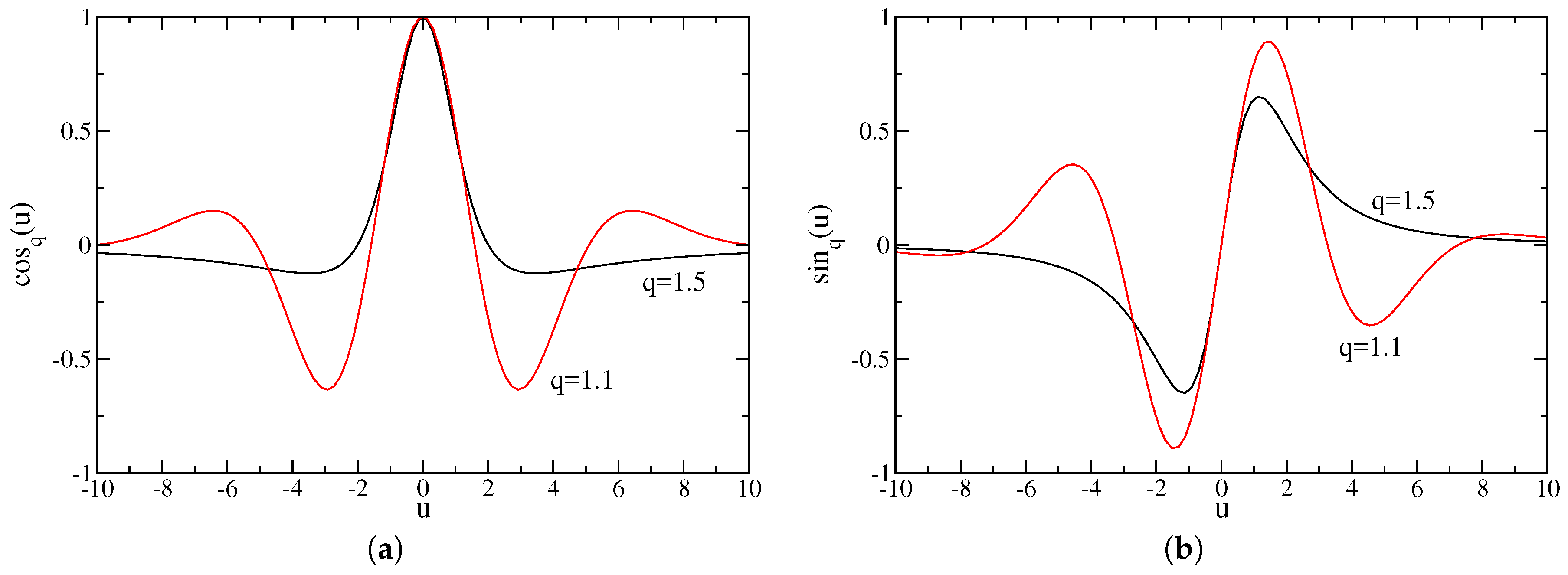
3.1. Free Particle and the q-Plane Wave Solution

Recently, a nonlinear Schroedinger equation (NLSE) for a free particle of mass m was proposed [67],

$$i\hslash \frac{\partial }{\partial t}\left[\frac{\mathsf{\Psi }(\overrightarrow{x},t)}{{\mathsf{\Psi }}_0}\right]=-\frac{1}{2-q}\frac{{\hslash }^2}{2m}{\nabla }^2{\left[\frac{\mathsf{\Psi }(\overrightarrow{x},t)}{{\mathsf{\Psi }}_0}\right]}^{2-q},$$

(23)

where q is a real number, as defined in Section 1, in such a way to recover the linear one of Equation (8), for $V\left(\overrightarrow{x}\right)=0$, in the particular case $q=1$. One sees that the right-hand side of this equation is nonlinear for any $q\ne 1$, so that, in contrast to Equation (8), the amplitude ${\mathsf{\Psi }}_0$ does not cancel and should be considered in these NL cases, guaranteeing the correct physical dimensionalities for all terms.

One should notice that the NLSE of Equation (23) presents the same structure of the NL Fokker–Planck equation proposed in [72,73] in the absence of an external potential, which appears in nonextensive statistical mechanics [6,9,10]. Essentially, it represents the analogue of the porous-medium equation [81], very common in the framework of anomalous-diffusion phenomena, but with an imaginary time.

Consistently, the energy and momentum operators are generalized as:

$$\widehat{E}=i\hslash D_t;{\widehat{p}}_n=-i\hslash D_{x_n};D_{u}f\left(u\right)\equiv {\left[f\left(u\right)\right]}^{1-q}df\left(u\right)/du,$$

(24)

which, when acting on the q-plane wave of Equation (6), yield the relations of Equation (11), namely those for the energy, $E=\hslash \omega$, and momentum, $\overrightarrow{p}=\hslash \overrightarrow{k}$. Now, considering $\overrightarrow{k}\to \overrightarrow{p}/\hslash$ and $\omega \to E/\hslash$, one verifies that this new form is a solution of the equation above, with $E=p^2/2m$, for all values of q.

Due to the peculiar properties of this type of solution, the q-generalized quantum mechanics is expected to be useful for addressing complex phenomena, such as dark matter, nonlinear quantum optics and others. In particular, some of the properties of the q-plane wave make it potentially relevant from the physical point of view, like: (i) it presents an oscillatory behavior; (ii) it is localized for certain values of q. Indeed, for $q\ne 1$, the q-exponential ${exp}_q\left(iu\right)$ is characterized by an amplitude $r_q\left(u\right)\ne 1$ [82],

$${exp}_q(\pm iu)={cos}_q\left(u\right)\pm i{sin}_q\left(u\right),$$

(25)

$${cos}_q\left(u\right)=r_q\left(u\right)cos\left\{\frac{1}{q-1}\arctan \left[(q-1)u\right]\right\},$$

(26)

$${sin}_q\left(u\right)=r_q\left(u\right)sin\left\{\frac{1}{q-1}\arctan \left[(q-1)u\right]\right\},$$

(27)

$$r_q\left(u\right)={\left[1+{(1-q)}^2{u}^2\right]}^{1/\left[2\right(1-q\left)\right]},$$

(28)

so that $r_q\left(u\right)$ decreases for increasing arguments, if $q>1$. From Equations (25)–(28), one notices that ${cos}_q\left(u\right)$ and ${sin}_q\left(u\right)$ cannot be zero simultaneously (even though their moduli do tend to zero simultaneously as $u\to \pm \infty$) yielding ${exp}_q(\pm iu)\ne 0$. In Figure 1, we represent ${cos}_q\left(u\right)$ and ${sin}_q\left(u\right)$, respectively, for two different values of $q>1$, showing that the amplitude $r_q\left(u\right)$ produces a modulation of these functions, which get strongly weakened as $\left|u\right|\to \infty$. Such a property makes these types of solutions appropriate for many types of physical phenomena, which occur in limited intervals of space and time. Let us stress that, in the particular situation where $\overrightarrow{k}·\overrightarrow{x}=\omega t$, one has $\mathsf{\Psi }(\overrightarrow{x},t)={\mathsf{\Psi }}_0(\forall t)$, and consequently, the q-plane wave behaves like a soliton. Indeed, in the one-dimensional case, one has a soliton propagating with a velocity $c=\omega /k$. This enables the approach of nonlinear excitations that do not deform in time and should be relevant, e.g., in nonlinear optics and plasma physics.

Additionally, ${exp}_q\left(iu\right)$ presents further peculiar properties,

$${\left[{exp}_q\left(iu\right)\right]}^{*}={exp}_q(-iu)={\left[1-(1-q)iu\right]}^{\frac{1}{1-q}},$$

(29)

$${exp}_q\left(iu\right){\left[{exp}_q\left(iu\right)\right]}^{*}={\left[r_q\left(u\right)\right]}^2={\left[1+{(1-q)}^2{u}^2\right]}^{\frac{1}{1-q}},$$

(30)

$${exp}_q\left(i{u}_1\right){exp}_q\left(i{u}_2\right)={exp}_q[i{u}_1+i{u}_2-(1-q)u_1{u}_2],$$

(31)

$${\left\{{\left[{exp}_q\left(iu\right)\right]}^{\alpha }\right\}}^{*}={\left\{{\left[{exp}_q\left(iu\right)\right]}^{*}\right\}}^{\alpha }={\left[{exp}_q(-iu)\right]}^{\alpha },$$

(32)

for any $\alpha \mathrm{real}$. By integrating Equation (30) from $-\infty$ to $+\infty$, one obtains [84],

$${\mathcal{I}}_q={\int }_{-\infty }^{\infty }du{\left[r_q\left(u\right)\right]}^2=\frac{\sqrt{\pi }\mathsf{\Gamma }\left(\frac{3-q}{2(q-1)}\right)}{(q-1)\mathsf{\Gamma }\left(\frac{1}{q-1}\right)},$$

(33)

leading to the physically-important property of square integrability for $1<q<3$; as some typical examples, one has ${\mathcal{I}}_{3/2}={\mathcal{I}}_2=\pi$. One should notice that this integral diverges in both limits $q\to 1$ and $q\to 3$. Hence, the q-plane wave of Equation (6) presents a modulation, characteristic of a localized wave, for $1<q<3$.

Applying the complex conjugate in Equation (23) and using the property of Equation (32), one obtains the equation for ${\mathsf{\Psi }}^{*}(\overrightarrow{x},t)$,

$$i\hslash \frac{\partial }{\partial t}\left[\frac{{\mathsf{\Psi }}^{*}(\overrightarrow{x},t)}{{\mathsf{\Psi }}_0}\right]=\frac{1}{2-q}\frac{{\hslash }^2}{2m}{\nabla }^2{\left[\frac{{\mathsf{\Psi }}^{*}(\overrightarrow{x},t)}{{\mathsf{\Psi }}_0}\right]}^{2-q}.$$

(34)

Next, we will discuss the subject of a probability density and its corresponding continuity equation, related to the present NLSE. As will be shown, this analysis turns out to be rather nontrivial, as examined in detail in [85,86].

3.2. Continuity Equation and Classical Field Theory

Let us now address the matter of the continuity equation; we start by following the standard procedure, i.e., considering the probability density of Equation (12), together with the pair of Equations (23) and (34). One has:

$$i\hslash \frac{\partial \rho (\overrightarrow{x},t)}{\partial t}=\frac{i\hslash }{\mathsf{\Omega }{\mathsf{\Psi }}_0^2}\left[\frac{\partial \mathsf{\Psi }(\overrightarrow{x},t)}{\partial t}{\mathsf{\Psi }}^{*}(\overrightarrow{x},t)+\mathsf{\Psi }(\overrightarrow{x},t)\frac{\partial {\mathsf{\Psi }}^{*}(\overrightarrow{x},t)}{\partial t}\right],$$

(35)

so that, using this pair of equations on the right-hand side, one readily sees that the continuity equation is not fulfilled. Instead, one gets the following balance equation:

$$\frac{\partial \rho (\overrightarrow{x},t)}{\partial t}+\overrightarrow{\nabla }·\overrightarrow{J}(\overrightarrow{x},t)=R(\overrightarrow{x},t),$$

(36)

where:

$$\overrightarrow{J}(\overrightarrow{x},t)=\frac{i\hslash }{2m\mathsf{\Omega }{\mathsf{\Psi }}_0^{3-q}}\left[-{\mathsf{\Psi }}^{1-q}(\overrightarrow{\nabla }\mathsf{\Psi }){\mathsf{\Psi }}^{*}+{({\mathsf{\Psi }}^{*})}^{1-q}(\overrightarrow{\nabla }{\mathsf{\Psi }}^{*})\mathsf{\Psi }\right],$$

(37)

$$R(\overrightarrow{x},t)=\frac{i\hslash }{2m\mathsf{\Omega }{\mathsf{\Psi }}_0^{3-q}}\left[-{\mathsf{\Psi }}^{1-q}(\overrightarrow{\nabla }\mathsf{\Psi })·(\overrightarrow{\nabla }{\mathsf{\Psi }}^{*})+{({\mathsf{\Psi }}^{*})}^{1-q}(\overrightarrow{\nabla }{\mathsf{\Psi }}^{*})·(\overrightarrow{\nabla }\mathsf{\Psi })\right].$$

(38)

These results show that the continuity equation of Equations (15) and (16) is recovered for $q=1$; in general, for $q\ne 1$, one has $R(\overrightarrow{x},t)\ne 0$. Indeed, considering the q-plane wave solution of Equation (6), one obtains:

$$R(\overrightarrow{x},t)=\frac{(1-q)\hslash }{m\mathsf{\Omega }}(\overrightarrow{k}·\overrightarrow{x}-\omega t)k^2{\left[1+{(1-q)}^2{(\overrightarrow{k}·\overrightarrow{x}-\omega t)}^2\right]}^{q/(1-q)},$$

(39)

showing that for $q\ne 1$, only in the particular case of the soliton, where $\overrightarrow{k}·\overrightarrow{x}=\omega t$ (leading to $\mathsf{\Psi }(\overrightarrow{x},t)={\mathsf{\Psi }}_0(\forall t)$), one has $R=0$, so that probability is preserved in time.

Moreover, one may see that by considering a Lagrangian density in the form of Equation (18), characterized by $\mathsf{\Psi }(\overrightarrow{x},t)$ and ${\mathsf{\Psi }}^{*}(\overrightarrow{x},t)$, and following a procedure similar to the one carried put in the linear case [78,79,80]), one does not obtain Equations (23) and (34). A way to overcome this difficulty was proposed in [85], where an additional field $\mathsf{\Phi }(\overrightarrow{x},t)$ was introduced. Hence, we will now develop an exact classical field theory, through the definition of a Lagrangian density $\mathcal{L}$, which will depend on the fields $\mathsf{\Psi }(\overrightarrow{x},t)$ and $\mathsf{\Phi }(\overrightarrow{x},t)$, their complex conjugates, as well as on their spatial and time derivatives,

$$\mathcal{L}\equiv \mathcal{L}\left(\mathsf{\Psi },\overrightarrow{\nabla }\mathsf{\Psi },\dot{\mathsf{\Psi }},\mathsf{\Phi },\overrightarrow{\nabla }\mathsf{\Phi },\dot{\mathsf{\Phi }},{\mathsf{\Psi }}^{*},\overrightarrow{\nabla }{\mathsf{\Psi }}^{*},{\dot{\mathsf{\Psi }}}^{*},{\mathsf{\Phi }}^{*},\overrightarrow{\nabla }{\mathsf{\Phi }}^{*},{\dot{\mathsf{\Phi }}}^{*}\right).$$

(40)

Let us then consider the following Lagrangian density,

$$\begin{array}{c}\begin{array}{c}\hfill \mathcal{L}=\frac{A}{{\mathsf{\Phi }}_0{\mathsf{\Psi }}_0}\left\{i\hslash \mathsf{\Phi }(\overrightarrow{x},t)\dot{\mathsf{\Psi }}(\overrightarrow{x},t)-\frac{{\hslash }^2}{2m}{\left[\frac{\mathsf{\Psi }(\overrightarrow{x},t)}{{\mathsf{\Psi }}_0}\right]}^{1-q}[\overrightarrow{\nabla }\mathsf{\Phi }(\overrightarrow{x},t)]·[\overrightarrow{\nabla }\mathsf{\Psi }(\overrightarrow{x},t)]\right.\\ \hfill -\left.i\hslash {\mathsf{\Phi }}^{*}(\overrightarrow{x},t){\dot{\mathsf{\Psi }}}^{*}(\overrightarrow{x},t)-\frac{{\hslash }^2}{2m}{\left[\frac{{\mathsf{\Psi }}^{*}(\overrightarrow{x},t)}{{\mathsf{\Psi }}_0}\right]}^{1-q}[\overrightarrow{\nabla }{\mathsf{\Phi }}^{*}(\overrightarrow{x},t)]·[\overrightarrow{\nabla }{\mathsf{\Psi }}^{*}(\overrightarrow{x},t)]\right\},\end{array}\end{array}$$

(41)

where $A\equiv 1/\left(2q\mathsf{\Omega }\right)$ is a multiplicative constant and, as before, ${\mathsf{\Psi }}_0$ and ${\mathsf{\Phi }}_0$ represent the amplitudes of the fields $\mathsf{\Psi }(\overrightarrow{x},t)$ and $\mathsf{\Phi }(\overrightarrow{x},t)$, respectively. One should notice that the Lagrangian density above recovers the one of Equation (19) in the particular case $q=1$.

From the above Lagrangian density, one may construct a classical action, which may be extremized to yield the Euler–Lagrange equations for each field [78,79,80]. The Euler–Lagrange equation for the field Φ,

$$\frac{\partial \mathcal{L}}{\partial \mathsf{\Phi }}-\overrightarrow{\nabla }·\left[\frac{\partial \mathcal{L}}{\partial (\overrightarrow{\nabla }\mathsf{\Phi })}\right]-\frac{\partial }{\partial t}\frac{\partial \mathcal{L}}{\partial \dot{\mathsf{\Phi }}}=0,$$

(42)

leads to:

$$i\hslash \frac{\partial \mathsf{\Psi }(\overrightarrow{x},t)}{\partial t}+\frac{{\hslash }^2}{2m}(1-q){\left[\mathsf{\Psi }(\overrightarrow{x},t)\right]}^{-q}{[\nabla \mathsf{\Psi }(\overrightarrow{x},t)]}^2+\frac{{\hslash }^2}{2m}{\left[\mathsf{\Psi }(\overrightarrow{x},t)\right]}^{1-q}{\nabla }^2\mathsf{\Psi }(\overrightarrow{x},t)=0,$$

(43)

which corresponds to the NLSE of Equation (23). Carrying out the same procedure for the field $\mathsf{\Psi }(\overrightarrow{x},t)$, one obtains,

$$i\hslash \frac{\partial \mathsf{\Phi }(\overrightarrow{x},t)}{\partial t}=\frac{{\hslash }^2}{2m}{\left[\mathsf{\Psi }(\overrightarrow{x},t)\right]}^{1-q}{\nabla }^2\mathsf{\Phi }(\overrightarrow{x},t),$$

(44)

with similar equations holding for the complex-conjugate fields, ${\mathsf{\Psi }}^{*}(\overrightarrow{x},t)$ and ${\mathsf{\Phi }}^{*}(\overrightarrow{x},t)$.

It is important to notice that Equation (44) becomes the complex conjugate of Equation (23) (i.e., Equation (34)) only for $q=1$, in which case $\mathsf{\Phi }(\overrightarrow{x},t)={\mathsf{\Psi }}^{*}(\overrightarrow{x},t)$. For all $q\ne 1$, one has that $\mathsf{\Phi }(\overrightarrow{x},t)$ is distinct from ${\mathsf{\Psi }}^{*}(\overrightarrow{x},t)$, with the fields $\mathsf{\Phi }(\overrightarrow{x},t)$ and $\mathsf{\Psi }(\overrightarrow{x},t)$ being related by Equation (44).

Now, if one substitutes the q-plane wave solution of Equation (6) in Equation (44), one finds,

$$\frac{\mathsf{\Phi }(\overrightarrow{x},t)}{{\mathsf{\Phi }}_0}={\left\{{exp}_q\left[i(\overrightarrow{k}·\overrightarrow{x}-\omega t)\right]\right\}}^{-q}={\left[\frac{\mathsf{\Psi }(\overrightarrow{x},t)}{{\mathsf{\Psi }}_0}\right]}^{-q}.$$

(45)

Consistently with the above, we generalize Equation (12) by defining the probability density for finding a particle at time t, in a given position $\overrightarrow{x}$, as:

$$\rho (\overrightarrow{x},t)=\frac{1}{2\mathsf{\Omega }{\mathsf{\Psi }}_0{\mathsf{\Phi }}_0}[\mathsf{\Psi }(\overrightarrow{x},t)\mathsf{\Phi }(\overrightarrow{x},t)+{\mathsf{\Psi }}^{*}(\overrightarrow{x},t){\mathsf{\Phi }}^{*}(\overrightarrow{x},t)],$$

(46)

for any value of q. Hence, considering the q-plane wave solution for a free particle, one has $\rho (\overrightarrow{x},t)=1/\mathsf{\Omega }$, leading trivially to $[\partial \rho (\overrightarrow{x},t)/\partial t]=0$, but yielding the same non-integrability difficulty of Equation (13), typical of the standard plane-wave solution in full space.

In fact, the continuity equation is fulfilled for this particular solution, although in general, one has:

$$\begin{array}{cc}& i\hslash \frac{\partial \rho (\overrightarrow{x},t)}{\partial t}=\frac{i\hslash }{2\mathsf{\Omega }{\mathsf{\Psi }}_0{\mathsf{\Phi }}_0}\left[\frac{\partial \mathsf{\Psi }(\overrightarrow{x},t)}{\partial t}\mathsf{\Phi }(\overrightarrow{x},t)+\mathsf{\Psi }(\overrightarrow{x},t)\frac{\partial \mathsf{\Phi }(\overrightarrow{x},t)}{\partial t}\right.\hfill \\ +& \left.\frac{\partial {\mathsf{\Psi }}^{*}(\overrightarrow{x},t)}{\partial t}{\mathsf{\Phi }}^{*}(\overrightarrow{x},t)+{\mathsf{\Psi }}^{*}(\overrightarrow{x},t)\frac{\partial {\mathsf{\Phi }}^{*}(\overrightarrow{x},t)}{\partial t}\right],\hfill \end{array}$$

(47)

and using the equations for the fields $\mathsf{\Psi }(\overrightarrow{x},t)$ and $\mathsf{\Phi }(\overrightarrow{x},t)$ (Equations (23) and (44)), as well as their corresponding complex conjugates, one obtains a balance equation in the form of Equation (36), where

$$\begin{array}{ccc}\hfill \overrightarrow{J}(\overrightarrow{x},t)& =& \frac{i\hslash }{4m\mathsf{\Omega }{\mathsf{\Psi }}_0^{2-q}{\mathsf{\Phi }}_0}\left[-{\mathsf{\Psi }}^{1-q}(\overrightarrow{\nabla }\mathsf{\Psi })\mathsf{\Phi }+{({\mathsf{\Psi }}^{*})}^{1-q}(\overrightarrow{\nabla }{\mathsf{\Psi }}^{*}){\mathsf{\Phi }}^{*}\right.\hfill \\ & +& \left.{\mathsf{\Psi }}^{2-q}(\overrightarrow{\nabla }\mathsf{\Phi })-{({\mathsf{\Psi }}^{*})}^{2-q}(\overrightarrow{\nabla }{\mathsf{\Phi }}^{*})\right],\hfill \end{array}$$

(48)

and

$$R(\overrightarrow{x},t)=\frac{i(1-q)\hslash }{4m\mathsf{\Omega }{\mathsf{\Psi }}_0^{2-q}{\mathsf{\Phi }}_0}\left[{\mathsf{\Psi }}^{1-q}(\overrightarrow{\nabla }\mathsf{\Psi })·(\overrightarrow{\nabla }\mathsf{\Phi })-{({\mathsf{\Psi }}^{*})}^{1-q}(\overrightarrow{\nabla }{\mathsf{\Psi }}^{*})·(\overrightarrow{\nabla }{\mathsf{\Phi }}^{*})\right].$$

(49)

One should notice that Equations (48) and (49) coincide with Equations (37) and (38), respectively, through the identifications $\mathsf{\Phi }(\overrightarrow{x},t)\leftrightarrow {\mathsf{\Psi }}^{*}(\overrightarrow{x},t)$ and ${\mathsf{\Phi }}^{*}(\overrightarrow{x},t)\leftrightarrow \mathsf{\Psi }(\overrightarrow{x},t)$. Therefore, within this later frame, solutions must satisfy:

$${[\mathsf{\Psi }(\overrightarrow{x},t)]}^{1-q}[\overrightarrow{\nabla }\mathsf{\Psi }(\overrightarrow{x},t)]·[\overrightarrow{\nabla }\mathsf{\Phi }(\overrightarrow{x},t)]\in \Re ,$$

(50)

for the preservation of probability. Since herein we are dealing with nonlinear equations, which usually present more than one solution, some possible solutions may not satisfy the above requirement for $q\ne 1$. Now, in contrast to Equation (38), considering the pair of solutions in Equations (6) and (45), one shows that:

$$\frac{1}{{\mathsf{\Psi }}_0^{2-q}{\mathsf{\Phi }}_0}[{\mathsf{\Psi }}^{1-q}(\overrightarrow{\nabla }\mathsf{\Psi })·(\overrightarrow{\nabla }\mathsf{\Phi })]=\frac{1}{{\mathsf{\Psi }}_0^{2-q}{\mathsf{\Phi }}_0}[{({\mathsf{\Psi }}^{*})}^{1-q}(\overrightarrow{\nabla }{\mathsf{\Psi }}^{*})·(\overrightarrow{\nabla }{\mathsf{\Phi }}^{*})]=q{k}^2\Rightarrow R(\overrightarrow{x},t)=0,$$

(51)

so that the continuity equation is fulfilled for the q-plane wave and its auxiliary solution of Equation (45). Next, we present other solutions for the pair of Equations (23) and (44); as will be shown, in many cases, the condition of Equation (50) is not fulfilled trivially.

3.3. Other Free-Particle Solutions and Approaches

3.3.1. Solutions with the Separation of Variables

Solutions characterized by the separation of variables have been worked out in [87,88] for the pair of Equations (23) and (44), whereas in [89], this kind of solution was developed for Equation (23) solely; these solutions are described briefly below. For simplicity, herein, we restrict ourselves to a one-dimensional space; these types of solutions are decomposed into spatial and temporal parts. Therefore, considering $\mathsf{\Psi }(x,t)={\psi }_1\left(x\right){\psi }_2\left(t\right)$ in Equation (23), one has [87,88,89]:

$$-\frac{{\hslash }^2}{2m(2-q)}\frac{{\psi }_{10}}{{\psi }_1\left(x\right)}\frac{d^2}{d{x}^2}{\left[\frac{{\psi }_1\left(x\right)}{{\psi }_{10}}\right]}^{2-q}=i\hslash {\left[\frac{{\psi }_{20}}{{\psi }_2\left(t\right)}\right]}^{2-q}\frac{d}{dt}\left[\frac{{\psi }_2\left(t\right)}{{\psi }_{20}}\right]=ϵ,$$

(52)

where ϵ is a constant with energy dimensions, whereas ${\psi }_{10}$ and ${\psi }_{20}$ represent the amplitudes of ${\psi }_1\left(x\right)$ and ${\psi }_2\left(t\right)$, respectively. Thus, we can write:

$$\frac{d^2}{d{x}^2}{\left[\frac{{\psi }_1\left(x\right)}{{\psi }_{10}}\right]}^{2-q}+ϵ\frac{2m(2-q)}{{\hslash }^2}\left[\frac{{\psi }_1\left(x\right)}{{\psi }_{10}}\right]=0,$$

(53)

and:

$$\frac{d}{dt}\left[\frac{{\psi }_2\left(t\right)}{{\psi }_{20}}\right]+i\frac{ϵ}{\hslash }{\left[\frac{{\psi }_2\left(t\right)}{{\psi }_{20}}\right]}^{2-q}=0.$$

(54)

By direct calculus, we find the expressions:

$${\psi }_1\left(x\right)={\psi }_{10}{exp}_{(q+1)/2}\left[i\sqrt{\frac{4mϵ}{(3-q){\hslash }^2}}x\right],$$

(55)

and:

$${\psi }_2\left(t\right)={\psi }_{20}{exp}_{2-q}\left[-iϵt/\hslash \right].$$

(56)

Now, we take into account Equations (55) and (56) to obtain:

$$\mathsf{\Psi }(x,t)={\mathsf{\Psi }}_0{\left[\frac{1+(1-q)ikx\sqrt{\frac{2}{3-q}}-{(1-q)}^2\frac{k^2{x}^2}{2(3-q)}}{1-(q-1)\frac{iϵt}{\hslash }}\right]}^{\frac{1}{1-q}}.$$

(57)

In particular, we emphasize that, in the limit of $q\to 1$, by keeping only terms of order $(q-1)$, the present decomposed solution coincides with the family of solutions given by q-plane waves $\mathsf{\Psi }(x,t)={\mathsf{\Psi }}_0{exp}_q\left[i(kx-wt)\right]$, in the same limit.

Following a similar procedure, the extra field can also be decomposed as $\mathsf{\Phi }(x,t)={\varphi }_1\left(x\right){\varphi }_2\left(t\right)$, so that substituting this solution in Equation (44), we obtain [87,88]:

$$-\frac{{\hslash }^2}{2m}\frac{{\varphi }_{10}}{{\varphi }_1\left(x\right)}{\left[\frac{{\psi }_1\left(x\right)}{{\psi }_{10}}\right]}^{1-q}\frac{d^2}{d{x}^2}\left[\frac{{\varphi }_1\left(x\right)}{{\varphi }_{10}}\right]=-i\hslash {\left[\frac{{\psi }_{20}}{{\psi }_2\left(t\right)}\right]}^{1-q}\frac{{\varphi }_{20}}{{\varphi }_2\left(t\right)}\frac{d}{dt}\left[\frac{{\varphi }_2\left(t\right)}{{\varphi }_{20}}\right]=\mu ,$$

(58)

where μ is a constant with energy dimensions. At this point, one should mention that two different solutions have been worked out, depending on the choices for the two energy parameters above, namely ϵ and μ. The first and simpler choice corresponds to $\mu =ϵ$ [87], which yields:

$$\left[\frac{{\varphi }_1\left(x\right)}{{\varphi }_{10}}\right]={\left[\frac{{\psi }_1\left(x\right)}{{\psi }_{10}}\right]}^{-1}\mathrm{and}\left[\frac{{\varphi }_2\left(t\right)}{{\varphi }_{20}}\right]={\left[\frac{{\psi }_2\left(t\right)}{{\psi }_{20}}\right]}^{-1},$$

(59)

so that this solution is also characterized by the probability density $\rho (x,t)=1/\mathsf{\Omega }$, for all values of q.

The solution explored in [88] considered the energies ϵ and μ as distinct, in principle. In this case, the equivalent to the equalities of Equation (59) is given by:

$$\left[\frac{{\varphi }_1\left(x\right)}{{\varphi }_{10}}\right]={\left[\frac{{\psi }_1\left(x\right)}{{\psi }_{10}}\right]}^{\gamma /2}\mathrm{and}\left[\frac{{\varphi }_2\left(t\right)}{{\varphi }_{20}}\right]={\left[\frac{{\psi }_2\left(t\right)}{{\psi }_{20}}\right]}^{-\mu /ϵ},$$

(60)

where γ is a real number, so that the two energies are related through:

$$\gamma (\gamma +q-1)ϵ=2(3-q)\mu ,$$

(61)

with the case $\mu =ϵ$, considered in [87], being recovered for $\gamma =-2$. Other choices for γ may lead to nontrivial probability densities $\rho (x,t)$, e.g., the choice $\gamma =q-3$, yielding $\mu =(2-q)ϵ$, results in a $\rho (x,t)$ integrable in a finite symmetric interval [88]. One should mention that considering $\mu \ne \epsilon$ seems to be a natural alternative, since these energies come from two distinct equations and may possibly be associated with two strongly correlated particles.

The extension of these results to the d-dimensional case is straightforward. We remind that the solutions for the pair of Equations (23) and (44) in d dimensions can also be decomposed into spatial and temporal parts. However, in contrast to the linear case, the spatial part cannot be decomposed into d different coordinate components.

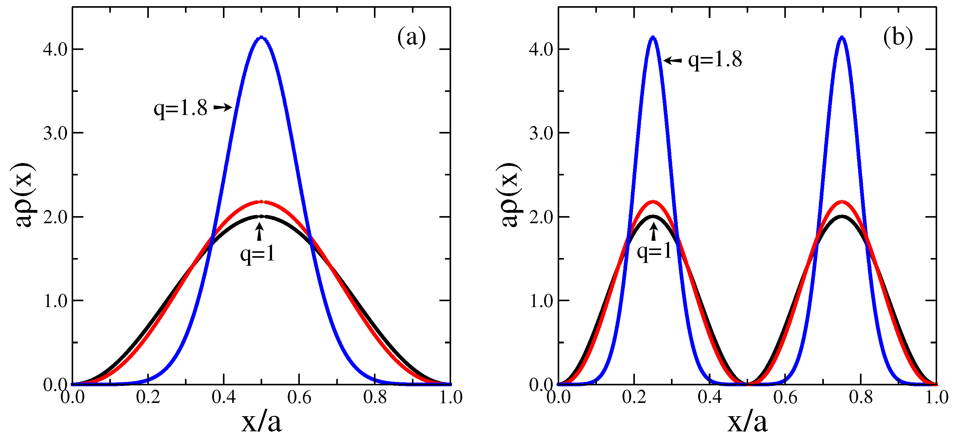
3.3.2. q-Gaussian Wave-Packet Solution

This type of solution was considered in [87,89,90,91,92,93], and it presents the convenience that it may be applied to both cases of a free particle [87,89,90,91,92], as well as for a particle under some particular potentials [91,93]. Herein, for simplicity, we will describe only the solution for the NLSE of Equation (23), i.e., a free particle, in a one-dimensional space. Accordingly, the following ansatz was proposed in [91],

$$\mathsf{\Psi }(x,t)={\mathsf{\Psi }}_0{\left\{1-(1-q)[a\left(t\right)x^2+b\left(t\right)x+c\left(t\right)]\right\}}^{1/(1-q)},$$

(62)

where the time dependence was introduced through the coefficients $a\left(t\right)$, $b\left(t\right)$, and $c\left(t\right)$, which may be complex, in general. By substituting this solution in Equation (23), one gets:

$$i\hslash \frac{\partial }{\partial t}\left[\frac{\mathsf{\Psi }(\overrightarrow{x},t)}{{\mathsf{\Psi }}_0}\right]=-i\hslash [\dot{a}\left(t\right)x^2+\dot{b}\left(t\right)x+\dot{c}\left(t\right)]{\left[\frac{\mathsf{\Psi }(\overrightarrow{x},t)}{{\mathsf{\Psi }}_0}\right]}^q,$$

(63)

so that $\dot{a}\left(t\right)$, $\dot{b}\left(t\right)$ and $\dot{c}\left(t\right)$ follow a set of three coupled ordinary differential equations.

One should notice that such a q-Gaussian wave-packet solution was considered for the pair of Equations (23) and (44) only in [87]. In this case, under particular conditions for the coefficients of Equation (62), the corresponding solution for the field $\mathsf{\Phi }(x,t)$ was shown to be related to $\mathsf{\Psi }(x,t)$ by means of a form similar to the one in Equation (45),

$$\frac{\mathsf{\Phi }(x,t)}{{\mathsf{\Phi }}_0}={\left[\frac{\mathsf{\Psi }(x,t)}{{\mathsf{\Psi }}_0}\right]}^{-q},$$

(64)

leading to $\rho (x,t)=1/\mathsf{\Omega }$ in Equation (46), so that $[\partial \rho (\overrightarrow{x},t)/\partial t]=0$, but with the same difficulty of Equation (13).

All other approaches analyzed the q-Gaussian wave-packet solution for Equation (23) only [89,90,91,92,93]. In these cases, the norm ${\left|\mathsf{\Psi }(x,t)\right|}^2$ is not preserved (see, e.g., the discussion of [91]).

3.3.3. Further Free-Particle Approaches

In the linear case, the pilot-wave theory, also known as the de Broglie–Bohm framework [94,95], represents an interpretation of great interest in quantum theory. This approach has been extended recently in [92], by considering Equation (23), as well as the probability density of Equation (12), for a free particle. In this case, the particle’s motion is governed by a velocity field ${\overrightarrow{v}}_q(\overrightarrow{x},t)$, determined by the time-dependent solution of Equation (23). Such a velocity field follows the balance equation of Equation (36), where $\overrightarrow{J}(\overrightarrow{x},t)=\rho (\overrightarrow{x},t){\overrightarrow{v}}_q(\overrightarrow{x},t)$, so that Equation (37) leads to:

$${\overrightarrow{v}}_q(\overrightarrow{x},t)=\frac{i\hslash }{2m\mathsf{\Omega }{\mathsf{\Psi }}_0^{1-q}}\left[-{\mathsf{\Psi }}^{-q}(\overrightarrow{\nabla }\mathsf{\Psi })+{({\mathsf{\Psi }}^{*})}^{-q}(\overrightarrow{\nabla }{\mathsf{\Psi }}^{*})\right].$$

(65)

The authors of [92] verified that, by considering the q-plane-wave solution of Equation (6), one finds the balance equation with $R(\overrightarrow{x},t)$ given by Equation (39), although the velocity field above yields:

$${\overrightarrow{v}}_q(\overrightarrow{x},t)=\frac{\hslash \overrightarrow{k}}{m};k=\sqrt{2m\omega };(\forall q),$$

(66)

preserving the same expression of the LSE. This remarkable result shows that the velocity field associated with the q-plane wave solution presents an invariant structure, independent of the parameter q.

Further traveling-wave solutions were found recently for the pair of Equations (23) and (44) in [88]; restricting to the one-dimensional case, for simplicity, such solutions were expressed as:

$$\begin{array}{ccc}\hfill \mathsf{\Psi }(x,t)& =& f\left(v\right)=f\left(i\right(kx-\omega t\left)\right),\hfill \end{array}$$

(67)

$$\begin{array}{ccc}\hfill \mathsf{\Phi }(x,t)& =& g\left(v\right)=g\left(i\right(kx-\omega t\left)\right),\hfill \end{array}$$

(68)

so that $v=iu=i(kx-\omega t)$. Substituting these solutions in Equations (23) and (44), one obtains two second-order ordinary differential equations, respectively,

$$\begin{array}{ccc}\hfill a\frac{df}{dv}& =& \frac{d}{dv}\left[f^{1-q}\frac{df}{dv}\right],\hfill \end{array}$$

(69)

$$\begin{array}{ccc}\hfill a\frac{dg}{dv}& =& -f^{1-q}\frac{d^{2}g}{d{v}^2},\hfill \end{array}$$

(70)

where:

$$a=\frac{2m\omega }{\hslash k^2}=\frac{\hslash \omega }{\left({\hslash }^2{k}^2\right)/\left(2m\right)}.$$

(71)

Integrating Equation (69), the first-order ordinary differential equation appears,

$$\frac{df}{dv}=a{f}^q+b{f}^{q-1},$$

(72)

where the integration quantity b is given by:

$$b={\left[f^{1-q}\left(v\right)\frac{df\left(v\right)}{dv}-af\left(v\right)\right]}_{v=0}.$$

(73)

It is important to recall that the dimensionless positive quantity a is given as the ratio of two important energies of the problem, namely the energy of a quantum of radiation $\hslash \omega$ (or, equivalently, the energy quantum of a one-dimensional harmonic oscillator) and the kinetic energy of the particle under investigation, $\left({\hslash }^2{k}^2\right)/\left(2m\right)$. Moreover, the dimensionless quantity b depends on a, as well as on the function $f\left(v\right)$ and its derivative at $v=0$.

Now, in Equation (72), one notices that the contribution $b{f}^{q-1}$ is irrelevant in the limit $q=1$, leading to the well-known plane-wave solution [1]. However, for $q\ne 1$, this term comes out naturally from the integration of the NLSE, written in the form of Equation (69). Herein, the q-plane wave solution is given by $f\left(v\right)={exp}_q\left(av\right)={exp}_q\left(iau\right)$, corresponding to the particular case $b=0$ in Equation (72). This is easily verified, since $(df\left(v\right)/dv)=a{[{exp}_q\left(av\right)]}^q$, so that one has $f\left(0\right)=1$ and ${(df\left(v\right)/dv)}_{v=0}=a$, yielding $b=0$ in Equation (73).

The analysis of the additional contribution $b{f}^{q-1}$ in the solution of the NLSE represented one of the main results of [88], in view of the changes it incurs to the q-plane wave solution. Due to this additional contribution, finding exact solutions became a hard task, in such a way that the solutions found in [88] were approximate, e.g., in the form of power series. Particularly, different limits were considered for the quantity b of Equation (73) in these power series, namely $a\gg \left|b\right|$ (representing a physical situation of low kinetic energies) and $a\ll \left|b\right|$ (representing a physical situation of high kinetic energies).

Furthermore, it should be mentioned that recent investigations have associated the q-exponential with a hypergeometric function, and consequently, the q-exponential should follow the hypergeometric differential equation [89,90]. In this way, the authors of [89,90] have derived the NLSE of Equation (23) by introducing transformations in the hypergeometric differential equation. This approach opened the possibility for the investigation of other differential equations that may be transformed in the hypergeometric differential equation, for which the q-exponential function appears as a solution.

3.4. Nonlinear Schroedinger Equations for a Particle in a Potential

The authors of [96] investigated how the q-plane wave solution of Equation (6) gets transformed under two basic types of changes in the reference frame, namely a Galilean transformation connecting two inertial reference frames, as well as the case of a uniformly-accelerated reference frame. In these transformations, we will restrict ourselves to a one-dimensional space, for simplicity, although the extension to d dimensions is straightforward. Hence, let us consider a Galilean transformation relating the original inertial frame $(x^{\prime },t^{\prime })$ with a second inertial frame $(x,t)$ that moves with respect to the former one with a uniform velocity v, so that:

$$t=t^{\prime };x=x^{\prime }-v{t}^{\prime }.$$

(74)

In this case, it was shown that the q-plane wave solution, in the second inertial frame $(x,t)$, keeps the form of Equation (6) by redefining the wave vector and frequency [96],

$$\tilde{k}=k-\frac{mv}{\hslash };\tilde{\omega }=\omega -kv+\frac{m{v}^2}{2\hslash }.$$

(75)

Furthermore, for a free particle viewed from a uniformly-accelerated reference frame (with acceleration a), the space-time coordinates are:

$$t=t^{\prime };x=x^{\prime }-\frac{a}{2}{t}^{\prime 2}=x^{\prime }-\frac{F}{2m}{t}^{\prime 2},$$

(76)

where, as before, $(x^{\prime },t^{\prime })$ represent the variables associated with the inertial frame, and $F=ma$ stands for the force acting on the particle. Such an analysis suggested that in the corresponding NLSE, the potential $V\left(x\right)$ should couple to ${\left[\mathsf{\Psi }(x,t)\right]}^q$, instead of coupling to $\mathsf{\Psi }(x,t)$, as happens in the standard LSE.

Taking into account the results of [96], the Lagrangian density for the free particle was modified by introducing a d-dimensional potential $V\left(\overrightarrow{x}\right)$ [78],

$$\mathcal{L}\equiv {\mathcal{L}}_{\mathrm{free}}-A\left\{V\left(\overrightarrow{x}\right)\left[\frac{\mathsf{\Phi }(\overrightarrow{x},t)}{{\mathsf{\Phi }}_0}\right]{\left[\frac{\mathsf{\Psi }(\overrightarrow{x},t)}{{\mathsf{\Psi }}_0}\right]}^q+V\left(\overrightarrow{x}\right)\left[\frac{{\mathsf{\Phi }}^{*}(\overrightarrow{x},t)}{{\mathsf{\Phi }}_0}\right]{\left[\frac{{\mathsf{\Psi }}^{*}(\overrightarrow{x},t)}{{\mathsf{\Psi }}_0}\right]}^q\right\},$$

(77)

where ${\mathcal{L}}_{\mathrm{free}}$ stands for the free-particle Lagrangian density of Equation (41), with the same constant factor A. Following the procedure described before [78,79,80], the Euler–Lagrange equation for the field $\mathsf{\Phi }(\overrightarrow{x},t)$ yields the NLSE:

$$i\hslash \frac{\partial }{\partial t}\left[\frac{\mathsf{\Psi }(\overrightarrow{x},t)}{{\mathsf{\Psi }}_0}\right]=-\frac{1}{2-q}\frac{{\hslash }^2}{2m}{\nabla }^2{\left[\frac{\mathsf{\Psi }(\overrightarrow{x},t)}{{\mathsf{\Psi }}_0}\right]}^{2-q}+V\left(\overrightarrow{x}\right){\left[\frac{\mathsf{\Psi }(\overrightarrow{x},t)}{{\mathsf{\Psi }}_0}\right]}^q,$$

(78)

whereas the Euler–Lagrange equation for the field $\mathsf{\Psi }(\overrightarrow{x},t)$ leads to the auxiliary equation,

$$i\hslash \frac{\partial }{\partial t}\left[\frac{\mathsf{\Phi }(\overrightarrow{x},t)}{{\mathsf{\Phi }}_0}\right]=\frac{{\hslash }^2}{2m}{\left[\frac{\mathsf{\Psi }(\overrightarrow{x},t)}{{\mathsf{\Psi }}_0}\right]}^{1-q}{\nabla }^2\left[\frac{\mathsf{\Phi }(\overrightarrow{x},t)}{{\mathsf{\Phi }}_0}\right]-qV\left(\overrightarrow{x}\right){\left[\frac{\mathsf{\Psi }(\overrightarrow{x},t)}{{\mathsf{\Psi }}_0}\right]}^{q-1}\left[\frac{\mathsf{\Phi }(\overrightarrow{x},t)}{{\mathsf{\Phi }}_0}\right].$$

(79)

An interesting feature concerning Equations (78) and (79) is that in the first of them, the potential $V\left(\overrightarrow{x}\right)$ appears multiplying ${\left[\mathsf{\Psi }(\overrightarrow{x},t)\right]}^q$, whereas in the second, it couples to ${\left[\mathsf{\Psi }(\overrightarrow{x},t)\right]}^{(q-1)}\mathsf{\Phi }(\overrightarrow{x},t)$. Considering these terms in the simple case of a constant potential, $V\left(\overrightarrow{x}\right)=V_0$, the q-plane wave of Equation (6) together with the solution for the second field $\mathsf{\Phi }(\overrightarrow{x},t)$ of Equation (45) satisfy both field equations, leading to $\hslash \omega ={\hslash }^2{k}^2/2m+V_0$, where $k^2={\sum }_{n=1}^d{k}_n^2$ in d dimensions.

To our knowledge, the first solutions of Equation (78) were presented in [91,97]: (i) the Gaussian wave-packet solution of Equation (62) was studied in [91] by considering a one-dimensional harmonic potential; (ii) solutions for several potentials were analyzed in [97], like the d-dimensional quadratic, the shifted-attractive delta and the two-dimensional Moshinsky ones. This latter potential is defined as:

$$V(x,y)=\frac{1}{2}{\omega }^2\left[x^2+y^2+\kappa {(x-y)}^2\right]-V_0,$$

(80)

and working with the center-of-mass coordinates,

$$R=\frac{1}{\sqrt{2}}(x+y);r=\frac{1}{\sqrt{2}}(x-y),$$

(81)

the authors of [97] have shown that Equation (78) admits the quasi-stationary solution:

$$\mathsf{\Psi }(R,r)=B{\left[1-(1-q)({\lambda }_1{R}^2+{\lambda }_2{r}^2)\right]}^{1/(1-q)}=B{exp}_q[{\lambda }_1{R}^2+{\lambda }_2{r}^2],$$

(82)

where the parameters ${\lambda }_1$ and ${\lambda }_2$ are related to ω, κ and B by means of two coupled nonlinear equations. The wave function of Equation (82) represents the first case reported in the literature of a solution of Equation (78) for a system of interacting particles. In the limit $q\to 1$, the solution above reduces to the ground-state function associated with the Moshinsky model’s potential.

An extension of the work of [97] was carried for the case where the particles are subjected to a Moshinsky-like potential with time-dependent coefficients [93]. In this latter work, the authors have shown that the nonlinearity creates entanglement between the particles, which is not present in the usual ($q=1$) scenario and, so, being potentially relevant for describing physical reality [95].

A common feature in the studies of [91,93,97] is the fact that by studying only Equation (78), the norm is not preserved, in the sense that the continuity given by Equation (15) is not fulfilled (for a discussion of the non-preservation of the norm, see, e.g., [91]). A joint study of Equations (78) and (79) was carried in [87], for a particle in an infinite one-dimensional rectangular potential well,

$$V\left(x\right)=\left\{\begin{array}{cc}0,\hfill & 0<x<a\hfill \\ \infty ,\hfill & \mathrm{otherwise}.\hfill \end{array}\right.$$

(83)

Hence, considering the same separation of variables of Subsection 3.3.1, i.e., $\mathsf{\Psi }(x,t)={\psi }_1\left(x\right){\psi }_2\left(t\right)$ and $\mathsf{\Phi }(x,t)={\varphi }_1\left(x\right){\varphi }_2\left(t\right)$, stationary-state solutions were found,

$${\psi }_1\left(x\right)={\psi }_{10}{\left[A_q{\mathrm{Sin}}_q(k_{q}x+\delta )\right]}^{\frac{1}{2-q}},$$

(84)

and by choosing $\mu =(2-q)ϵ$,

$${\varphi }_1\left(x\right)={\left[{\psi }_1\left(x\right)\right]}^{2-q}.$$

(85)

The stationary-state solutions for this potential were expressed in terms of $y={\mathrm{Sin}}_q\left(x\right)$, defined by means of [87]:

$$x\equiv {\mathrm{Sin}}_q^{-1}\left(y\right)={\int }_0^y\frac{dz}{\sqrt{1-z^{\frac{3-q}{2-q}}}},$$

(86)

whose period is $4{\tau }_q$, where:

$${\tau }_q={\int }_0^1\frac{dz}{\sqrt{1-z^{\frac{3-q}{2-q}}}}=\sqrt{\pi }\frac{(2-q)\mathsf{\Gamma }\left(\right(2-q)/(3-q\left)\right)}{(3-q)\mathsf{\Gamma }\left(\right(7-3q)/(6-2q\left)\right)}.$$

(87)

The equations above express a generalization of the standard trigonometric function, recovered in the limit $q=1$, i.e., ${\mathrm{Sin}}_1\left(x\right)\equiv sin\left(x\right)$. One should notice that this generalization differs from the ${sin}_q\left(x\right)$ function that is currently used in nonextensive statistics [82]; particularly, one important distinction concerns the fact that $|{\mathrm{Sin}}_q\left(x\right)|\le 1$ for $1\le q<2$ [87]. In this way, the wave vectors in Equation (84) are given by:

$$k_q\equiv \sqrt{2}{\left(\frac{2mϵ{(2-q)}^2}{(3-q){\hslash }^2}\right)}^{\frac{2-q}{3-q}},$$

(88)

and considering the boundary condition ${\psi }_1\left(0\right)={\psi }_1\left(a\right)=0$, one finds $\delta =0$ and $k_{q}a=2{\tau }_{q}n$, where $n=1,2,3,..$, so that:

$${\psi }_1\left(x\right)={\psi }_1(x,q,n)={\left[{\tilde{A}}_{q,n}{\mathrm{Sin}}_q\left(\frac{2n{\tau }_{q}x}{a}\right)\right]}^{\frac{1}{2-q}}.$$

(89)

Then, the following expression:

$${ϵ}_n\left(q\right)=\frac{(3-q){\hslash }^2}{2m{(2-q)}^2}{\left(\frac{\sqrt{2}n{\tau }_q}{a}\right)}^{\frac{3-q}{2-q}},$$

(90)

generalizes the energy spectrum of the standard quantum well, ${ϵ}_n\left(1\right)=({\hslash }^2/2m){(n\pi /a)}^2$.

Finally, we can write the probability density of Equation (46) as:

$$\rho \left(x\right)=\frac{\mathrm{Re}\left\{{\left[{\mathrm{Sin}}_q(2n{\tau }_{q}x/a)\right]}^{\frac{3-q}{2-q}}\right\}}{a{\int }_0^{1}dx\mathrm{Re}\left\{{\left[{\mathrm{Sin}}_q(2n{\tau }_{q}x/a)\right]}^{\frac{3-q}{2-q}}\right\}},$$

(91)

where $\mathrm{Re}\left\{s\right\}$ stands for the real part of s, and we have used the normalization condition for finding the amplitude ${\tilde{A}}_{n,q}$. It is important to stress that $\mathrm{Re}\{{\left[{\mathrm{Sin}}_q(2n{\tau }_{q}x/a)\right]}^{(3-q)/(2-q)}\}>0$ for $1<q<4/3$ and that this quantity may be also positive for other values of q outside this interval, e.g., whenever the parameter q satisfies the inequalities $(3/2)+2k<(3-q)/(2-q)<(5/2)+2k$, with k integer and $k\ge 1$. However, there are values of q in the range $4/3<q<2$ for which one obtains $\rho \left(x\right)<0$, representing situations still not well understood. Such cases may be compared with what happens to the Wigner function, which may present negative values for some values of its arguments, and so, it cannot be considered as a simple probability distribution, being often called a quasidistribution (see, e.g., [98]).

In Figure 2, we present the dimensionless probability density $a\rho \left(x\right)$, for a particle in an infinite potential well (cf. Equation (83)) in the cases $n=1$ (a) and $n=2$ (b) and typical values of q, namely $q=1,1.25$ and $1.8$. For $n=1$, one has an argument $0\le (2{\tau }_{q}x/a)\le 2{\tau }_q$, so that ${\mathrm{Sin}}_q(2{\tau }_{q}x/a)\ge 0$ [87]. From Figure 2a, one notices that q plays an important role for a particle with an energy ${ϵ}_1\left(q\right)$, as concerns its confinement around the central region of the well: by increasing q in the range $1<q<2$, the particle becomes more confined around $(x/a)=1/2$. In this context, the present solution with an index $q>1$ may be relevant for systems where one finds a low-energy particle localized in the central region of a confining potential. In Figure 2b, we show $a\rho \left(x\right)$ in the case $n=2$ and the same values of q considered in Figure 2a. Now, one has an argument $0\le (4{\tau }_{q}x/a)\le 4{\tau }_q$, so that ${\mathrm{Sin}}_q(4{\tau }_{q}x/a)$ may yield negative values for $(x/a)>1/2$ [87]. As mentioned above, in these cases, one has always real positive probabilities for $1<q<4/3$, as well as other values of q outside this interval (e.g., $q=1.8$). In these cases, the corresponding probability densities present a symmetry with respect to $(x/a)=1/2$, with maxima at $(x/a)=1/4$ and $(x/a)=3/4$. Once again, the present solution with an index $q>1$ may be relevant for systems where one finds a low-energy particle with the same probability for being found in two different regions, symmetrically localized around the central region of the well.

4. Linear Nonhomogeneous Proposals of the Schroedinger Equation

A linear Schroedinger equation with position-dependent effective masses, the linear nonhomogeneous Schroedinger equation (LNHSE), has attracted the attention of many workers recently [99,100,101,102,103,104,105,106,107,108,109,110]. These research works were motivated by the fact that a wide variety of physical systems are well described through this type of equation, like semiconductor heterostructures [99,100], polarons [101], quantum wells and quantum dots [102], among others.

The particular type of dependence of the mass on the position, i.e., the form of the function $m=m\left(x\right)$ (in the one-dimensional case), may change according to the physical interest, and in some cases, the resulting equation, although linear, is intimately related to the NLSE of the previous section. Particularly, the additional wave function used to construct a consistent continuity equation of the NLSE appears to be necessary also for some LNHSEs [105,106,110], introducing an extra difficulty, since one has an additional equation of motion with which to deal. It is then natural to try to understand deeply the need for the introduction of this additional wave function (or field) and to search a proper way to work with it. In general, the LNHSEs are simpler to deal with, becoming appropriate for a better understanding of the necessity of an additional wave function, which will be discussed next.

In [105,106], it was realized that certain LNHSEs had to be properly approached by the introduction of an additional wave function, similarly to the NLSE considered previously here. However, it is important to notice how the construction of a consistent continuity equation for this latter case leads to a direct clue to connect both fields. Herein, we will follow the general treatment given in [110], which covers a wide family of position-dependent mass Hamiltonians considered previously in the literature. Let us start by considering one-dimensional position-dependent mass Hamiltonians, depending on a real function $f[m\left(x\right),m^{\prime }\left(x\right)]$, where the general position-dependent mass $m\left(x\right)$ is an analytical positive function for any value of x, and $m^{\prime }\left(x\right)$ represents its first derivative; such a Hamiltonian is defined by:

$$\widehat{H}=\frac{-{\hslash }^2}{2m\left(x\right)}\frac{{\partial }^2}{\partial x^2}+\frac{{\hslash }^2}{2}\alpha f[m\left(x\right),m^{\prime }\left(x\right)]\frac{\partial }{\partial x}+V\left(x\right),$$

(92)

where $\alpha \in \mathbb{R}$ is a dimensionless constant and $V\left(x\right)$ stands for a general potential. These class of Hamiltonians lead to Schroedinger equations, which are not, in general, self-adjoint in the usual Hilbert space of their eigenfunctions. In what follows, we show the conditions for Equation (92) to be self-adjoint.

Let us now introduce a Lagrangian density, which reproduces easily the equation of motion for the above Hamiltonian,

$$\begin{array}{c}\hfill \mathcal{L}=\frac{i\hslash }{2}\mathsf{\Phi }(x,t)\frac{\partial \mathsf{\Psi }(x,t)}{\partial t}+\frac{{\hslash }^2}{4m\left(x\right)}\mathsf{\Phi }(x,t)\frac{{\partial }^2\mathsf{\Psi }(x,t)}{\partial x^2}-\frac{{\hslash }^2\alpha }{4}f(m,m^{\prime })\mathsf{\Phi }(x,t)\frac{\partial \mathsf{\Psi }(x,t)}{\partial x}\\ \hfill -\frac{i\hslash }{2}{\mathsf{\Phi }}^{*}(x,t)\frac{\partial {\mathsf{\Psi }}^{*}(x,t)}{\partial t}+\frac{{\hslash }^2}{4m\left(x\right)}{\mathsf{\Phi }}^{*}(x,t)\frac{{\partial }^2{\mathsf{\Psi }}^{*}(x,t)}{\partial x^2}-\frac{{\hslash }^2\alpha }{4}f(m,m^{\prime }){\mathsf{\Phi }}^{*}(x,t)\frac{\partial {\mathsf{\Psi }}^{*}(x,t)}{\partial x}\\ \hfill -\frac{1}{2}V{\mathsf{\Phi }}^{*}(x,t){\mathsf{\Psi }}^{*}(x,t)-\frac{1}{2}V\left(x\right)\mathsf{\Phi }(x,t)\mathsf{\Psi }(x,t).\end{array}$$

(93)

Using the usual Euler–Lagrange equations for the fields $\mathsf{\Phi }(x,t)$ and its conjugate, one straightforwardly gets the corresponding Schroedinger equations,

$$\begin{array}{cc}\hfill i\hslash \frac{\partial \mathsf{\Psi }(x,t)}{\partial t}& =-\frac{{\hslash }^2}{2m\left(x\right)}\frac{{\partial }^2\mathsf{\Psi }(x,t)}{\partial x^2}+\frac{{\hslash }^2}{2}\alpha f(m,m^{\prime })\frac{d\mathsf{\Psi }(x,t)}{dx}+V\left(x\right)\mathsf{\Psi }(x,t)\hfill \end{array}$$

(94)

$$\begin{array}{cc}\hfill -i\hslash \frac{\partial {\mathsf{\Psi }}^{*}(x,t)}{\partial t}& =-\frac{{\hslash }^2}{2m\left(x\right)}\frac{{\partial }^2{\mathsf{\Psi }}^{*}(x,t)}{\partial x^2}+\frac{{\hslash }^2}{2}\alpha f(m,m^{\prime })\frac{d{\mathsf{\Psi }}^{*}(x,t)}{dx}+V\left(x\right){\mathsf{\Psi }}^{*}(x,t).\hfill \end{array}$$

(95)

In order to obtain the equations for the fields $\mathsf{\Phi }(x,t)$ and ${\mathsf{\Phi }}^{*}(x,t)$ one must take into account the Euler–Lagrange equation that includes a second derivative term [111,112], e.g., the one for the field $\mathsf{\Psi }(x,t)$,

$$\frac{\partial \mathcal{L}}{\partial \mathsf{\Psi }}-\frac{\partial }{\partial x}\left[\frac{\partial \mathcal{L}}{\partial (\partial \mathsf{\Psi }/\partial x)}\right]-\frac{\partial }{\partial t}\left[\frac{\partial \mathcal{L}}{\partial (\partial \mathsf{\Psi }/\partial t)}\right]+\frac{{\partial }^2}{\partial x^2}\left[\frac{\partial \mathcal{L}}{\partial ({\partial }^2\mathsf{\Psi }/\partial x^2)}\right]=0,$$

(96)

leading to:

$$\begin{array}{cc}\hfill -i\hslash \frac{\partial \mathsf{\Phi }(x,t)}{\partial t}& =-\frac{{\hslash }^2}{2}\frac{{\partial }^2}{\partial x^2}\left(\frac{\mathsf{\Phi }(x,t)}{m\left(x\right)}\right)-\frac{{\hslash }^2\alpha }{2}\frac{\partial }{\partial x}\left[f(m,m^{\prime })\mathsf{\Phi }(x,t)\right]+V\left(x\right)\mathsf{\Phi }(x,t)\hfill \end{array}$$

(97)

$$\begin{array}{cc}\hfill i\hslash \frac{\partial {\mathsf{\Phi }}^{*}(x,t)}{\partial t}& =-\frac{{\hslash }^2}{2}\frac{{\partial }^2}{\partial x^2}\left(\frac{{\mathsf{\Phi }}^{*}(x,t)}{m\left(x\right)}\right)-\frac{{\hslash }^2\alpha }{2}\frac{\partial }{\partial x}\left[f(m,m^{\prime }){\mathsf{\Phi }}^{*}(x,t)\right]+V\left(x\right){\mathsf{\Phi }}^{*}(x,t).\hfill \end{array}$$

(98)

Note that in the case of a constant mass, $\mathsf{\Phi }(x,t)={\mathsf{\Psi }}^{*}(x,t)$, and only one field is necessary, so that Equations (94) and (95) are the same as Equations (98) and (97), respectively; however, in general, one has $\mathsf{\Phi }(x,t)\ne {\mathsf{\Psi }}^{*}(x,t)$.

The Continuity Equation

Similarly to Equation (46), herein one defines the function $\rho (x,t)$ as:

$$\rho (x,t)=\frac{1}{2m_0}\left[\mathsf{\Psi }(x,t)\mathsf{\Phi }(x,t)+{\mathsf{\Psi }}^{*}(x,t){\mathsf{\Phi }}^{*}(x,t)\right],$$

(99)

where $m_0$ represents a constant with dimensions of mass, and we are restricting ourselves to systems for which the integral of $\rho (x,t)$ (cf. Equation (13)) over the whole space is finite. Let us then consider the following ansatz,

$$\mathsf{\Phi }(x,t)=g\left(x\right)m\left(x\right){\mathsf{\Psi }}^{*}(x,t),$$

(100)

where we require $g\left(x\right)$ to be positive definite. Hence, using the Schroedinger Equations (94) and (97), it is simple to show that the above-defined probability density obeys the one-dimensional continuity equation (cf. Equation (15)), with the following current density,

$$J(x,t)=\frac{\hslash }{2i{m}_0}g\left(x\right)\left[\frac{\partial \mathsf{\Psi }(x,t)}{\partial x}{\mathsf{\Phi }}^{*}(x,t)-\mathsf{\Psi }(x,t)\frac{\partial {\mathsf{\Psi }}^{*}(x,t)}{\partial x}\right],$$

(101)

and as a consequence, the function $g\left(x\right)$ should satisfy:

$$\frac{dg\left(x\right)}{dx}=-\alpha f(m,m^{\prime })m\left(x\right)g\left(x\right).$$

(102)

Moreover, inspired by the form that the probability density $\rho (x,t)=\frac{1}{m_0}g\left(x\right)m\left(x\right)\mathsf{\Psi }(x,t){\mathsf{\Psi }}^{*}(x,t)$, one defines the inner product:

$$\langle {\mathsf{\Psi }}_1(x,t),{\mathsf{\Psi }}_2(x,t)\rangle =\int dxg\left(x\right)m\left(x\right){\mathsf{\Psi }}_1^{*}(x,t){\mathsf{\Psi }}_2(x,t),$$

(103)

and averages should be now computed using this form for the inner product. Considering this inner product, the Hamiltonian given in Equation (92) can be shown to be self-adjoint. One sees that from the linear nonhomogeneous systems defined in this section, one of the essential consequences of removing the additional field is a new recipe for computing mean values. In [110], it was also shown that forms of the operators likewise change, being in general different from the cases with the standard inner product.

It is important to mention that the NLSE of the previous section is far more complicated than the LNHSE considered above. Nevertheless, it is possible that in certain nonlinear cases, there may exist appropriate transformations, like the one of Equation (100), connecting the fields Φ and Ψ. It would be interesting to investigate the possibility of finding such a transformation for the NLSE of the previous section and to analyze its consequences.

5. Generalized Nonlinear Klein–Gordon Equation

In [67], besides the NLSE of Section 3, other nonlinear generalized quantum equations were introduced, like proposals for the Klein–Gordon and Dirac equations. In this section, we will discuss briefly the nonlinear Klein–Gordon equation (NLKGE) introduced in [67], which for a particle of mass m in d dimensions is given by:

$${\nabla }^2\left[\frac{\mathsf{\Psi }(\overrightarrow{x},t)}{{\mathsf{\Psi }}_0}\right]=\frac{1}{c^2}\frac{{\partial }^2}{\partial t^2}\left[\frac{\mathsf{\Psi }(\overrightarrow{x},t)}{{\mathsf{\Psi }}_0}\right]+q\frac{m^2{c}^2}{{\hslash }^2}{\left[\frac{\mathsf{\Psi }(\overrightarrow{x},t)}{{\mathsf{\Psi }}_0}\right]}^{2q-1},$$

(104)

recovering the standard linear Klein–Gordon equation in the case $q=1$ [78]. One may verify that the q-plane wave of Equation (6) satisfies the NLKGE above, preserving the corresponding energy-momentum relation for all q,

$$E^2=p^2{c}^2+m^2{c}^4.$$

(105)

Although Equation (104) and its solution in Equation (6) are valid for a general d-dimensional position vector $\overrightarrow{x}$, herein, for simplicity, we will restrict ourselves to a three-dimensional vector $\overrightarrow{x}$; let us then introduce the four-dimensional space-time operators [78,79,80],

$${\partial }^{\mu }\equiv \frac{\partial }{\partial x_{\mu }}\equiv \left\{\frac{\partial }{\partial \left(ct\right)},-\frac{\partial }{\partial x},-\frac{\partial }{\partial y},-\frac{\partial }{\partial z}\right\};{\partial }_{\mu }\equiv \frac{\partial }{\partial x^{\mu }}\equiv \left\{\frac{\partial }{\partial \left(ct\right)},\frac{\partial }{\partial x},\frac{\partial }{\partial y},\frac{\partial }{\partial z}\right\},$$

(106)

so that Equation (104) may be rewritten as:

$${\partial }^{\mu }{\partial }_{\mu }\left[\frac{\mathsf{\Psi }(\overrightarrow{x},t)}{{\mathsf{\Psi }}_0}\right]+q\frac{m^2{c}^2}{{\hslash }^2}{\left[\frac{\mathsf{\Psi }(\overrightarrow{x},t)}{{\mathsf{\Psi }}_0}\right]}^{2q-1}=0.$$

(107)

Similarly to the NLSE [85], a classical field theory was introduced for the NLKGE in [86]. This approach was also developed in terms of two classical fields, $\mathsf{\Psi }(\overrightarrow{x},t)$ and $\mathsf{\Phi }(\overrightarrow{x},t)$, by writing the following Lagrangian density,

$$\begin{array}{c}\begin{array}{c}\hfill \mathcal{L}=\frac{\tilde{A}}{{\mathsf{\Phi }}_0{\mathsf{\Psi }}_0}\left\{\mathsf{\Phi }(\overrightarrow{x},t)\left[{\partial }^{\mu }{\partial }_{\mu }\mathsf{\Psi }(\overrightarrow{x},t)\right]+q\frac{m^2{c}^2}{{\hslash }^2}\mathsf{\Phi }(\overrightarrow{x},t)\mathsf{\Psi }(\overrightarrow{x},t){\left[\frac{\mathsf{\Psi }(\overrightarrow{x},t)}{{\mathsf{\Psi }}_0}\right]}^{2(q-1)}\right.\\ \hfill +\left.{\mathsf{\Phi }}^{*}(\overrightarrow{x},t)\left[{\partial }^{\mu }{\partial }_{\mu }{\mathsf{\Psi }}^{*}(\overrightarrow{x},t)\right]+q\frac{m^2{c}^2}{{\hslash }^2}{\mathsf{\Phi }}^{*}(\overrightarrow{x},t){\mathsf{\Psi }}^{*}(\overrightarrow{x},t){\left[\frac{{\mathsf{\Psi }}^{*}(\overrightarrow{x},t)}{{\mathsf{\Psi }}_0}\right]}^{2(q-1)}\right\},\end{array}\end{array}$$

(108)

with the multiplicative factor, $\tilde{A}\equiv {\hslash }^2{c}^2/\left[2(1-3q)E\mathsf{\Omega }\right]$, depending on the total energy E, and as usual, the fields $\mathsf{\Psi }(\overrightarrow{x},t)$ and $\mathsf{\Phi }(\overrightarrow{x},t)$ are confined to a finite volume Ω [78]. The Lagrangian above is equivalent to:

$$\begin{array}{c}\hfill \mathcal{L}=\frac{\tilde{A}}{{\mathsf{\Phi }}_0{\mathsf{\Psi }}_0}\left\{-\left[{\partial }_{\mu }\mathsf{\Phi }(\overrightarrow{x},t)\right]\left[{\partial }^{\mu }\mathsf{\Psi }(\overrightarrow{x},t)\right]+q\frac{m^2{c}^2}{{\hslash }^2}\mathsf{\Phi }(\overrightarrow{x},t)\mathsf{\Psi }(\overrightarrow{x},t){\left[\frac{\mathsf{\Psi }(\overrightarrow{x},t)}{{\mathsf{\Psi }}_0}\right]}^{2(q-1)}\right.\\ \hfill +{\partial }_{\mu }\left[\mathsf{\Phi }(\overrightarrow{x},t){\partial }^{\mu }\mathsf{\Psi }(\overrightarrow{x},t)\right]-\left[{\partial }_{\mu }{\mathsf{\Phi }}^{*}(\overrightarrow{x},t)\right]\left[{\partial }^{\mu }{\mathsf{\Psi }}^{*}(\overrightarrow{x},t)\right]+q\frac{m^2{c}^2}{{\hslash }^2}\\ \hfill {\mathsf{\Phi }}^{*}(\overrightarrow{x},t){\mathsf{\Psi }}^{*}(\overrightarrow{x},t){\left[\frac{{\mathsf{\Psi }}^{*}(\overrightarrow{x},t)}{{\mathsf{\Psi }}_0}\right]}^{2(q-1)}+{\partial }_{\mu }\left[{\mathsf{\Phi }}^{*}(\overrightarrow{x},t){\partial }^{\mu }{\mathsf{\Psi }}^{*}(\overrightarrow{x},t)\right]\},\end{array}$$

(109)

where the total derivative terms are relevant for $q\ne 1$ (contrary to what happens in the linear case) [86]. One should notice that the above Lagrangian density presents higher-order derivatives, as compared to the one of Equation (41), i.e., it depends on the fields $\mathsf{\Psi }(\overrightarrow{x},t)$ and $\mathsf{\Phi }(\overrightarrow{x},t)$, as well as on their first and second derivatives,

$$\mathcal{L}\equiv \mathcal{L}\left(\mathsf{\Psi },{\partial }_{\mu }\mathsf{\Psi },{\partial }_{\mu }{\partial }_{\nu }\mathsf{\Psi },\mathsf{\Phi },{\partial }_{\mu }\mathsf{\Phi },{\partial }_{\mu }{\partial }_{\nu }\mathsf{\Phi },{\mathsf{\Psi }}^{*},{\partial }_{\mu }{\mathsf{\Psi }}^{*},{\partial }_{\mu }{\partial }_{\nu }{\mathsf{\Psi }}^{*},{\mathsf{\Phi }}^{*},{\partial }_{\mu }{\mathsf{\Phi }}^{*},{\partial }_{\mu }{\partial }_{\nu }{\mathsf{\Phi }}^{*}\right).$$

(110)

In this case, the Euler–Lagrange equations should take into account higher-order terms, in such a way that for the field Φ, one has [111,112],

$$\frac{\partial \mathcal{L}}{\partial \mathsf{\Phi }}-{\partial }_{\mu }\left[\frac{\partial \mathcal{L}}{\partial \left({\partial }_{\mu }\mathsf{\Phi }\right)}\right]+{\partial }_{\mu }{\partial }_{\nu }\left[\frac{\partial \mathcal{L}}{\partial \left({\partial }_{\mu }{\partial }_{\nu }\mathsf{\Phi }\right)}\right]=0.$$

(111)

Substituting the Lagrangian density of Equation (109) in the above Euler–Lagrange equation, one obtains the NLKGE of Equation (107); carrying out the same procedure in the Euler–Lagrange equation for the field Ψ,

$$\frac{\partial \mathcal{L}}{\partial \mathsf{\Psi }}-{\partial }_{\mu }\left[\frac{\partial \mathcal{L}}{\partial \left({\partial }_{\mu }\mathsf{\Psi }\right)}\right]+{\partial }_{\mu }{\partial }_{\nu }\left[\frac{\partial \mathcal{L}}{\partial \left({\partial }_{\mu }{\partial }_{\nu }\mathsf{\Psi }\right)}\right]=0,$$

(112)

one obtains an additional equation for the field Φ,

$${\nabla }^2\mathsf{\Phi }(\overrightarrow{x},t)=\frac{1}{c^2}\frac{{\partial }^2\mathsf{\Phi }(\overrightarrow{x},t)}{\partial t^2}+q(2q-1)\frac{m^2{c}^2}{{\hslash }^2}\mathsf{\Phi }(\overrightarrow{x},t){\left[\frac{\mathsf{\Psi }(\overrightarrow{x},t)}{{\mathsf{\Psi }}_0}\right]}^{2(q-1)}.$$

(113)

The equation above becomes the complex conjugate of Equation (104) for $q\to 1$ through the identification $\mathsf{\Phi }(\overrightarrow{x},t)={\mathsf{\Psi }}^{*}(\overrightarrow{x},t)$; substituting the q-exponential of Equation (6) in Equation (113), one finds,

$$\frac{\mathsf{\Phi }(\overrightarrow{x},t)}{{\mathsf{\Phi }}_0}={\left\{{exp}_q\left[\frac{i}{\hslash }(\overrightarrow{p}·\overrightarrow{x}-Et)\right]\right\}}^{-(2q-1)}={\left[\frac{\mathsf{\Psi }(\overrightarrow{x},t)}{{\mathsf{\Psi }}_0}\right]}^{-(2q-1)}.$$

(114)

One important aspect of Equation (113) may be seen by substituting the above solutions for $\mathsf{\Psi }(\overrightarrow{x},t)$ and $\mathsf{\Phi }(\overrightarrow{x},t)$ in order to reproduce the same energy-momentum relation of Equation (105), for all q.

The NLKGE of Equation (104) has attracted some interest recently, and it was shown to be directly related to the hypergeometric differential equation, being derived from the latter, through mathematical manipulations [90]. Moreover, by introducing a dissipative term in Equation (104), a nonlinear generalization of the celebrated telegraph equation was proposed [113].

6. Conclusions and Perspectives

Inspired by q-statistics, new types of nonlinear quantum equations were proposed recently, which included the Schroedinger, Klein–Gordon and Dirac equations for a free particle. These generalizations present nonlinear terms, characterized by exponents depending on an index q, in such a way that the standard linear equations are recovered in the limit $q\to 1$. This review focused mostly on recent advances for the nonlinear Schroedinger equation, although some results obtained for the Klein–Gordon and for a class of linear nonhomogeneous Schroedinger equations were also discussed.

Interestingly, in the case of a free particle, the nonlinear equations discussed herein present a common, soliton-like, traveling solution, which is written in terms of the q-exponential function that naturally emerges within nonextensive statistical mechanics. Such a solution, called the q-plane wave, preserves the corresponding well-known Einstein energy-momentum relation in both the Schroedinger and Klein–Gordon cases, for arbitrary values of q; in the first case, the Planck and the de Broglie relations are also preserved. Other solutions found recently in the literature for the nonlinear Schroedinger in both cases of a free particle, as well as for a particle in the presence of well-known potentials were also discussed. In this latter case, for an infinite potential well, solutions were found that may be relevant for systems where one finds a low-energy particle localized in the central region of a confining potential.

A common difficulty in all of these equations concerns the necessity for an additional field (or extra wave function) in order to fulfill the continuity equation. This conclusion was reached by means of a classical field theory, showing that besides the usual $\mathsf{\Psi }(\overrightarrow{x},t)$, a new field $\mathsf{\Phi }(\overrightarrow{x},t)$ should be introduced; this latter field becomes ${\mathsf{\Psi }}^{*}(\overrightarrow{x},t)$ only when $q\to 1$.

A class of linear nonhomogeneous Schroedinger equations, characterized by position-dependent masses, which need the extra field $\mathsf{\Phi }(\overrightarrow{x},t)$ in order to fulfill a continuity equation, is also discussed. Interestingly, in this case, an appropriate transformation connecting $\mathsf{\Psi }(\overrightarrow{x},t)$ and $\mathsf{\Phi }(\overrightarrow{x},t)$ was proposed, leading to the possibility for finding a connection between these fields in the nonlinear cases, which remains as an open problem.

Finally, the solutions presented herein are potential candidates for applications to nonlinear excitations in many physical systems, like plasmas, nonlinear optics, graphene structures, as well as in shallow and deep water waves.

References

1. Liboff, R.L. Introductory Quantum Mehanics, 4th ed.; Addison Wesley: San Francisco, CA, USA, 2003. [Google Scholar]
2. Merzbacher, E. Quantum Mehanics, 3rd ed.; John Wiley and Sons: New York, NY, USA, 1998. [Google Scholar]
3. Balian, R. From Microphysics to Macrophysics, vols. I and II; Springer: Berlin/Heidelberg, Germany, 1991. [Google Scholar]
4. Reichl, L.E. A Modern Course in Statistical Physics, 2nd ed.; Wiley: New York, NY, USA, 1998. [Google Scholar]
5. Tsallis, C. Possible generalization of Boltzmann–Gibbs statistics. J. Stat. Phys. 1988, 52, 479–487. [Google Scholar] [CrossRef]
6. Tsallis, C. Introduction to Nonextensive Statistical Mechanics; Springer: New York, NY, USA, 2009. [Google Scholar]
7. Curado, E.M.F.; Tsallis, C. Generalized statistical mechanics: Connection with thermodynamics. J. Phys. A 1991, 24, 3187, correction in 1992, 25, 1019. [Google Scholar] [CrossRef]
8. Tsallis, C.; Mendes, R.S.; Plastino, A.R. The role of constraints within generalized nonextensive statistics. Physica A 1998, 261, 534–554. [Google Scholar] [CrossRef]
9. Tsallis, C. Nonadditive entropy and nonextensive statistical mechanics—An overview after 20 years. Braz. J. Phys. 2009, 39, 337–356. [Google Scholar] [CrossRef]
10. Tsallis, C. An introduction to nonadditive entropies and a thermostatistical approach to inanimate and living matter. Contemp. Phys. 2014, 55, 179–197. [Google Scholar] [CrossRef]
11. Anteneodo, C.; Tsallis, C. Breakdown of exponential sensitivity to initial conditions: Role of the range of interactions. Phys. Rev. Lett. 1998, 80, 5313. [Google Scholar] [CrossRef]
12. Chavanis, P.-H.; Campa, A. Inhomogeneous Tsallis distributions in the hmf model. Eur. Phys. J. B 2010, 76, 581–611. [Google Scholar] [CrossRef]
13. Cirto, L.J.L.; Assis, V.R.V.; Tsallis, C. Influence of the interaction range on the thermostatistics of a classical many-body system. Physica A 2014, 393, 286–296. [Google Scholar] [CrossRef]
14. Christodoulidi, H.; Tsallis, C.; Bountis, T. Fermi-Pasta-Ulam model with long-range interactions: Dynamics and thermostatistics. Europhys. Lett. 2014, 108, 40006. [Google Scholar] [CrossRef]
15. Baldovin, F.; Robledo, A. Universal renormalization-group dynamics at the onset of chaos in logistic maps and nonextensive statistical mechanics. Phys. Rev. E 2002, 66, R045104. [Google Scholar] [CrossRef] [PubMed]
16. Baldovin, F.; Robledo, A. Nonextensive Pesin identity. Exact renormalization group analytical results for the dynamics at the edge of chaos of the logistic map. Phys. Rev. E 2004, 69, R045202. [Google Scholar] [CrossRef] [PubMed]
17. Mayoral, E.; Robledo, A. Tsallis’ q index and Mori’s q phase transitions at edge of chaos. Phys. Rev. E 2005, 72, 026209. [Google Scholar] [CrossRef] [PubMed]
18. Tirnakli, U.; Tsallis, C.; Beck, C. A closer look at time averages of the logistic map at the edge of chaos. Phys. Rev. E 2009, 79, 056209. [Google Scholar] [CrossRef] [PubMed]
19. Luque, B.; Lacasa, L.; Robledo, A. Feigenbaum graphs at the onset of chaos. Phys. Lett. A 2012, 376, 3625–3629. [Google Scholar] [CrossRef]
20. Douglas, P.; Bergamini, S.; Renzoni, F. Tunable Tsallis distributions in dissipative optical lattices. Phys. Rev. Lett. 2006, 96, 110601. [Google Scholar] [CrossRef] [PubMed]
21. Bagci, G.B.; Tirnakli, U. Self-organization in dissipative optical lattices. Chaos 2009, 19, 033113. [Google Scholar] [CrossRef] [PubMed]
22. Lutz, E.; Renzoni, F. Beyond Boltzmann-Gibbs statistical mechanics in optical lattices. Nat. Phys. 2013, 9, 615–619. [Google Scholar] [CrossRef]
23. Liu, B.; Goree, J. Superdiffusion and non-Gaussian statistics in a driven-dissipative 2D dusty plasma. Phys. Rev. Lett. 2008, 100, 055003. [Google Scholar] [CrossRef] [PubMed]
24. Bouzit, O.; Gougam, L.A.; Tribeche, M. Screening and sheath formation in a nonequilibrium mixed Cairns-Tsallis electron distribution. Phys. Plasmas 2015, 22, 052112. [Google Scholar] [CrossRef]
25. DeVoe, R.G. Power-law distributions for a trapped ion interacting with a classical buffer gas. Phys. Rev. Lett. 2009, 102, 063001. [Google Scholar] [CrossRef] [PubMed]
26. Pickup, R.M.; Cywinski, R.; Pappas, C.; Farago, B.; Fouquet, P. Generalized spin glass relaxation. Phys. Rev. Lett. 2009, 102, 097202. [Google Scholar] [CrossRef] [PubMed]
27. Tsallis, C.; de Souza, A.M.C.; Maynard, R. Derivation of Lévy-type anomalous superdiffusion from generalized statistical mechanics. In Lévy Flights and Related Topics in Physics; Shlesinger, M.F., Zaslavsky, G.M., Frisch, U., Eds.; Springer: Berlin/Heidelberg, Germany, 1995; p. 269. [Google Scholar]
28. Tsallis, C.; Levy, S.V.F.; de Souza, A.M.C.; Maynard, R. Statistical-mechanical foundation of the ubiquity of Levy distributions in nature. Phys. Rev. Lett. 1996, 75, 3589. [Google Scholar] [CrossRef] [PubMed]
29. Combe, G.; Richefeu, V.; Stasiak, M.; Atman, A.P.F. Experimental validation of nonextensive scaling law in confined granular media. Phys. Rev. Lett. 2015, 115, 238301. [Google Scholar] [CrossRef] [PubMed]
30. CMS Collaboration. Transverse-momentum and pseudorapidity distributions of charged hadrons in pp collisions at s = 0.9 and 2.36 TeV. J. High Energy Phys. 2010, 2, 041. [Google Scholar]
31. CMS Collaboration. Transverse-momentum and pseudorapidity distributions of charged hadrons in pp collisions at s = 7 TeV. Phys. Rev. Lett. 2010, 105, 022002. [Google Scholar]
32. Marques, L.; Andrade-II, E.; Deppman, A. Nonextensivity of hadronic systems. Phys. Rev. D 2013, 87, 114022. [Google Scholar] [CrossRef]
33. Marques, L.; Cleymans, J.; Deppman, A. Description of high-energy pp collisions using Tsallis thermodynamics: Transverse momentum and rapidity distributions. Phys. Rev. D 2015, 91, 054025. [Google Scholar] [CrossRef]
34. Oliveira, H.P.; Soares, I.D. Dynamics of black hole formation: Evidence for nonextensivity. Phys. Rev. D 2005, 71, 124034. [Google Scholar] [CrossRef]
35. Komatsu, N.; Kimura, S. Entropic cosmology for a generalized black-hole entropy. Phys. Rev. D 2013, 88, 083534. [Google Scholar] [CrossRef]
36. Silva, V.H.C.; Aquilanti, V.; de Oliveira, H.C.B.; Mundim, K.C. Uniform description of non-Arrhenius temperature dependence of reaction rates, and a heuristic criterion for quantum tunneling vs. classical non-extensive distribution. Chem. Phys. Lett. 2013, 590, 201–207. [Google Scholar] [CrossRef]
37. Borland, L. Closed form option pricing formulas based on a non-Gaussian stock price model with statistical feedback. Phys. Rev. Lett. 2002, 89, 098701. [Google Scholar] [CrossRef] [PubMed]
38. Ludescher, J.; Tsallis, C.; Bunde, A. Universal behaviour of interoccurrence times between losses in financial markets: An analytical description. Europhys. Lett. 2011, 95, 68002. [Google Scholar] [CrossRef]
39. Ludescher, J.; Bunde, A. Universal behavior of the interoccurrence times between losses in financial markets: Independence of the time resolution. Phys. Rev. 2014, 90, 062809. [Google Scholar] [CrossRef] [PubMed]
40. Antonopoulos, C.G.; Michas, G.; Vallianatos, F.; Bountis, T. Evidence of q-exponential statistics in Greek seismicity. Physica A 2014, 409, 71–77. [Google Scholar] [CrossRef]
41. Upadhyaya, A.; Rieu, J.-P.; Glazier, J.A.; Sawada, Y. Anomalous diffusion and non-Gaussian velocity distribution of Hydra cells in cellular aggregates. Physica A 2001, 293, 549–558. [Google Scholar] [CrossRef]
42. Bogachev, M.I.; Kayumov, A.R.; Bunde, A. Universal internucleotide statistics in full genomes: A footprint of the DNA structure and packaging? PLoS ONE 2014, 9, e112534. [Google Scholar] [CrossRef] [PubMed]
43. Burlaga, L.F.; Vinas, A.F. Triangle for the entropic index q of non-extensive statistical mechanics observed by Voyager 1 in the distant heliosphere. Physica A 2005, 356, 375–384. [Google Scholar] [CrossRef]
44. Burlaga, L.F.; Ness, N.F. Magnetic field strength fluctuations and the q-triplet in the heliosheath: Voyager 2 observations from 91.0 to 94.2 AU at latitude 30 S. Astrophys. J. 2013, 765, 35. [Google Scholar] [CrossRef]
45. Moyano, L.G.; Tsallis, C.; Gell-Mann, M. Numerical indications of a q-generalised central limit theorem. Europhys. Lett. 2006, 73, 813. [Google Scholar] [CrossRef]
46. Thistleton, W.J.; Marsh, J.A.; Nelson, K.P.; Tsallis, C. q-Gaussian approximants mimic non-extensive statistical-mechanical expectation for many-body probabilistic model with long-range correlations. Cent. Eur. J. Phys. 2009, 7, 387–394. [Google Scholar] [CrossRef]
47. Chavanis, P.-H. Nonlinear mean field Fokker-Planck equations. Application to the chemotaxis of biological population. Eur. Phys. J. B 2008, 62, 179–208. [Google Scholar] [CrossRef]
48. Umarov, S.; Tsallis, C.; Steinberg, S. On a q-central limit theorem consistent with nonextensive statistical mechanics. Milan J. Math. 2008, 76, 307–328. [Google Scholar] [CrossRef]
49. Queiros, S.M.D.; Tsallis, C. Nonextensive statistical mechanics and central limit theorems II—Convolution of q-independent random variables. In Complexity, Metastability and Nonextensivity; Abe, S., Herrmann, H.J., Quarati, P., Rapisarda, A., Tsallis, C., Eds.; AIP Publishing: New York, NY, USA, 2007. [Google Scholar]
50. Umarov, S.; Tsallis, C.; Gell-Mann, M.; Steinberg, S. Generalization of symmetric α-stable Lévy distributions for q > 1. J. Math. Phys. 2010, 51, 033502. [Google Scholar] [CrossRef] [PubMed]
51. Nelson, K.P.; Umarov, S. Nonlinear statistical coupling. Physica A 2010, 389, 2157–2163. [Google Scholar] [CrossRef]
52. Hanel, R.; Thurner, S.; Tsallis, C. Limit distributions of scale-invariant probabilistic models of correlated random variables with the q-Gaussian as an explicit example. Eur. Phys. J. B 2009, 72, 263–268. [Google Scholar] [CrossRef]
53. Umarov, S.; Tsallis, C. The limit distribution in the q-CLT for q ≥ 1 is unique and can not have a compact support. J. Phys. A 2016, 49, 415204. [Google Scholar] [CrossRef]
54. Caruso, F.; Tsallis, C. Nonadditive entropy reconciles the area law in quantum systems with classical thermodynamics. Phys. Rev. E 2008, 78, 021102. [Google Scholar] [CrossRef] [PubMed]
55. Carrasco, J.A.; Finkel, F.; Gonzalez-Lopez, A.; Rodriguez, M.A.; Tempesta, P. Generalized isotropic Lipkin-Meshkov-Glick models: Ground state entanglement and quantum entropies. J. Stat. Mech. 2016, 2016, 033114. [Google Scholar] [CrossRef]
56. Weinstein, Y.S.; Lloyd, S.; Tsallis, C. Border between between regular and chaotic quantum dynamics. Phys. Rev. Lett. 2002, 89, 214101. [Google Scholar] [CrossRef] [PubMed]
57. Betzler, A.S.; Borges, E.P. Nonextensive distributions of asteroid rotation periods and diameters. Astron. Astrophys. 2012, 539, A158. [Google Scholar] [CrossRef]
58. Betzler, A.S.; Borges, E.P. Nonextensive statistical analysis of meteor showers and lunar flashes. Mon. Not. R. Astron. Soc. 2015, 447, 765–771. [Google Scholar] [CrossRef]
59. Capurro, A.; Diambra, L.; Lorenzo, D.; Macadar, O.; Martin, M.T.; Mostaccio, C.; Plastino, A.; Rofman, E.; Torres, M.E.; Velluti, J. Tsallis entropy and cortical dynamics: The analysis of EEG signals. Physica A 1998, 257, 149–155. [Google Scholar] [CrossRef]
60. Mohanalin, J.; Beenamol; Kalra, P.K.; Kumar, N. A novel automatic microcalcification detection technique using Tsallis entropy and a type II fuzzy index. Comput. Math. Appl. 2010, 60, 2426–2432. [Google Scholar] [CrossRef]
61. Nivanen, L.; Le Mehaute, A.; Wang, Q.A. Generalized algebra within a nonextensive statistics. Rep. Math. Phys. 2003, 52, 437–444. [Google Scholar] [CrossRef]
62. Borges, E.P. A possible deformed algebra and calculus inspired in nonextensive thermostatistics. Physica A 2004, 340, 95–101. [Google Scholar] [CrossRef]
63. Tempesta, P. Group entropies, correlation laws, and zeta functions. Phys. Rev. E 2011, 84, 021121. [Google Scholar] [CrossRef] [PubMed]
64. Ruiz, G.; Tsallis, C. Reply to comment on “towards a large deviation theory for strongly correlated systems”. Phys. Lett. A 2013, 377, 491–495. [Google Scholar] [CrossRef]
65. Soares, D.J.B.; Tsallis, C.; Mariz, A.M.; Silva, L.R. Preferential attachment growth model and nonextensive statistical mechanics. Europhys. Lett. 2005, 70, 70. [Google Scholar] [CrossRef]
66. Brito, S.G.A.; da Silva, L.R.; Tsallis, C. Role of dimensionality in complex networks. Nat. Sci. Rep. 2016, 6, 27992. [Google Scholar] [CrossRef] [PubMed]
67. Nobre, F.D.; Rego-Monteiro, M.A.; Tsallis, C. Nonlinear Relativistic and Quantum Equations with a Common Type of Solution. Phys. Rev. Lett. 2011, 106, 140601. [Google Scholar] [CrossRef] [PubMed]
68. Scott, A.C. (Ed.) Encyclopedia of Nonlinear Science; Taylor and Francis: New York, NY, USA, 2005.
69. Scott, A.C. The Nonlinear Universe; Springer: Berlin/Heidelberg, Germany, 2007. [Google Scholar]
70. Polyanin, A.D.; Zaitsev, V.F. Handbook of Nonlinear Partial Differential Equations; Chapman and Hall—CRC: Boca Raton, FL, USA, 2004. [Google Scholar]
71. Frank, T.D. Nonlinear Fokker-Planck Equations: Fundamentals and Applications; Springer: Berlin/Heidelberg, Germany, 2005. [Google Scholar]
72. Plastino, A.R.; Plastino, A. Non-extensive statistical mechanics and generalized Fokker-Planck equation. Physica A 1995, 222, 347–354. [Google Scholar] [CrossRef]
73. Tsallis, C.; Bukman, D.J. Anomalous diffusion in the presence of external forces: Exact time-dependent solutions and their thermostatistical basis. Phys. Rev. E 1996, 54, R2197. [Google Scholar] [CrossRef]
74. Schwämmle, V.; Nobre, F.D.; Curado, E.M.F. Consequences of the H theorem from nonlinear Fokker-Planck equations. Phys. Rev. E 2007, 76, 041123. [Google Scholar] [CrossRef] [PubMed]
75. Schwämmle, V.; Curado, E.M.F.; Nobre, F.D. A general nonlinear Fokker-Planck equation and its associated entropy. Eur. Phys. J. B 2007, 58, 159–165. [Google Scholar] [CrossRef]
76. Ribeiro, M.S.; Nobre, F.D.; Curado, E.M.F. Classes of N-Dimensional Nonlinear Fokker-Planck Equations Associated to Tsallis Entropy. Entropy 2011, 13, 1928–1944. [Google Scholar] [CrossRef]
77. Sulem, C.; Sulem, P.-L. The Nonlinear Schroedinger Equation: Self-Focusing and Wave Collapse; Springer: New York, NY, USA, 1999. [Google Scholar]
78. Greiner, W. Relativistic Quantum Mechanics, 3rd ed.; Springer: Berlin/Heidelberg, Germany, 2000. [Google Scholar]
79. Greiner, W.; Reinhardt, J. Field Quantization; Springer: Berlin/Heidelberg, Germany, 1996. [Google Scholar]
80. Huang, K. Quantum Field Theory—From Operators to Path Integrals; WILEY-VCH: Weinheim, Germany, 2004. [Google Scholar]
81. Vázquez, J.L. The Porous Medium Equation; Oxford University Press: Oxford, UK, 2007. [Google Scholar]
82. Borges, E.P. On a q-generalization of circular and hyperbolic functions. J. Phys. A 1998, 31, 5281. [Google Scholar] [CrossRef]
83. Nobre, F.D.; Plastino, A.R. Generalized nonlinear Proca equation and its free-particle solutions. Eur. Phys. J. C 2016, 76, 343. [Google Scholar] [CrossRef]
84. Jauregui, M.; Tsallis, C. New representations of π and Dirac delta using the nonextensive-statistical- mechanics q-exponential function. J. Math. Phys. 2010, 51, 063304. [Google Scholar] [CrossRef]
85. Nobre, F.D.; Rego-Monteiro, M.A.; Tsallis, C. A generalized nonlinear Schroedinger equation: Classical field-theoretic approach. Europhys. Lett. 2012, 97, 41001. [Google Scholar] [CrossRef]
86. Rego-Monteiro, M.A.; Nobre, F.D. Nonlinear quantum equations: Classical field theory. J. Math. Phys. 2013, 54, 103302. [Google Scholar] [CrossRef]
87. Plastino, A.R.; Souza, A.M.C.; Nobre, F.D.; Tsallis, C. Stationary and uniformly accelerated states in nonlinear quantum mechanics. Phys. Rev. A 2014, 90, 062134. [Google Scholar] [CrossRef]
88. Bountis, T.; Nobre, F.D. Travelling-wave and separated variable solutions of a nonlinear Schroedinger equation. J. Math. Phys. 2016, 57, 082106. [Google Scholar] [CrossRef]
89. Plastino, A.; Rocca, M.C. From the hypergeometric differential equation to a non-linear Schroedinger one. Phys. Lett. A 2015, 379, 2690–2693. [Google Scholar] [CrossRef]
90. Plastino, A.; Rocca, M.C. Hypergeometric connotations of quantum equations. Physica A 2016, 450, 435–443. [Google Scholar] [CrossRef]
91. Curilef, S.; Plastino, A.R.; Plastino, A. Tsallis’ maximum entropy ansatz leading to exact analytical time dependent wave packet solutions of a nonlinear Schroedinger equation. Physica A 2013, 392, 2631–2642. [Google Scholar] [CrossRef]
92. Pennini, F.; Plastino, A.R.; Plastino, A. Pilot wave approach to the NRT nonlinear Schroedinger equation. Physica A 2014, 403, 195–205. [Google Scholar] [CrossRef]
93. Alves, L.G.A.; Ribeiro, H.V.; Santos, M.A.F.; Mendes, R.S.; Lenzi, E.K. Solutions for a q-generalized Schroedinger equation of entangled interacting particles. Physica A 2015, 429, 35–44. [Google Scholar] [CrossRef]
94. Holland, P.R. The Quantum Theory of Motion; Cambridge University Press: Cambridge, UK, 1993. [Google Scholar]
95. Bell, J.S. Speakable and Unspeakable in Quantum Mechanics; Cambridge University Press: Cambridge, UK, 1987. [Google Scholar]
96. Plastino, A.R.; Tsallis, C. Nonlinear Schroedinger equation in the presence of uniform acceleration. J. Math. Phys. 2013, 54, 041505. [Google Scholar] [CrossRef]
97. Toranzo, I.V.; Plastino, A.R.; Dehesa, J.S.; Plastino, A. Quasi-stationary states of the NRT nonlinear Schroedinger equation. Physica A 2013, 392, 3945–3951. [Google Scholar] [CrossRef]
98. Case, W.B. Wigner functions and Weyl transforms for pedestrians. Am. J. Phys. 2008, 76, 937–946. [Google Scholar] [CrossRef]
99. Bastard, G. Wave Mechanics Applied to Semiconductor Heterostructures; Les Editions de Physique: Les Ulis, France, 1988. [Google Scholar]
100. Weisbuch, C.; Vinter, B. Quantum Semiconductor Structures: Fundamentals and Applications; Academic Press: New York, NY, USA, 1991. [Google Scholar]
101. Zhao, F.Q.; Liang, X.X.; Ban, S.L. Influence of the spatially dependent effective mass on bound polarons in finite parabolic quantum wells. Eur. Phys. J. B 2003, 33, 3–8. [Google Scholar] [CrossRef]
102. Keshavarz, A.; Zamani, N. Optical properties of spherical quantum dot with position-dependent effective mass. Superlattices Microstruct. 2013, 58, 191–197. [Google Scholar] [CrossRef]
103. Plastino, A.R.; Rigo, A.; Casas, M.; Garcias, F.; Plastino, A. Supersymmetric approach to quantum systems with position-dependent effective mass. Phys. Rev. A 1999, 60, 4318. [Google Scholar] [CrossRef]
104. Costa Filho, R.N.; Almeida, M.P.; Farias, G.A.; Andrade, J.S., Jr. Displacement operator for quantum systems with position-dependent mass. Phys. Rev. A 2011, 84, 050102. [Google Scholar] [CrossRef]
105. Rego-Monteiro, M.A.; Nobre, F.D. Classical field theory for a non-Hermitian Schroedinger equation with position-dependent masses. Phys. Rev. A 2013, 88, 032105. [Google Scholar] [CrossRef]
106. Nobre, F.D.; Rego-Monteiro, M.A. Non-Hermitian PT Symmetric Hamiltonian with Position-Dependent Masses: Associated Schroedinger Equation and Finite-Norm Solutions. Braz. J. Phys. 2015, 45, 79–88. [Google Scholar] [CrossRef]
107. Costa Filho, R.N.; Alencar, G.; Skagerstam, B.-S.; Andrade, J.S., Jr. Morse potential derived from first principles. Europhys. Lett. 2013, 101, 10009. [Google Scholar] [CrossRef]
108. Sinha, A.; Roychoudhury, R. Scattering in a spatially varying mass-symmetric double heterojunction. Europhys. Lett. 2013, 103, 50007. [Google Scholar] [CrossRef]
109. Da Costa, B.G.; Borges, E.P. Generalized space and linear momentum operators in quantum mechanics. J. Math. Phys. 2014, 55, 062105. [Google Scholar] [CrossRef]
110. Rego-Monteiro, M.A.; Rodrigues, L.M.C.S.; Curado, E.M.F. Position-dependent mass quantum Hamiltonians: General approach and duality. J. Phys. A Math. Theor. 2016, 49, 125203. [Google Scholar] [CrossRef]
111. Bollini, C.G.; Giambiagi, J.J. Lagrangian Procedures for Higher Order Field Equations. Rev. Bras. Fís. 1987, 17, 14. [Google Scholar]
112. Barcelos-Neto, J.; Braga, N.R.F. Higher Order Canonical Formalism for the Scalar Field Theory. Acta Phys. Polonica B 1989, 20, 205–210. [Google Scholar]
113. Plastino, A.R.; Tsallis, C. Dissipative effects in nonlinear Klein-Gordon dynamics. Europhys. Lett. 2016, 113, 50005. [Google Scholar] [CrossRef]
Figure 1. Plots of the real and complex parts of exp q ( i u ) , i.e., cos q ( u ) (panel (a)) and sin q ( u ) (panel (b)), respectively, for two different values of q > 1 (cf. Equations (25)–(28)). Due to the amplitude r q ( u ) = 1 + ( 1 q ) 2 u 2 1 / [ 2 ( 1 q ) ] , the oscillatory behavior is strongly depressed for increasing values of q. All quantities exhibited are dimensionless (from [83]).
Entropy 19 00039 g001
Figure 2. The dimensionless probability density a ρ ( x ) (cf. Equation (91)), for a particle in a one-dimensional infinite potential well of size a, is represented for typical values of q, namely, q = 1 , 1 . 25 and 1 . 8 (from bottom to top), in the cases n = 1 (a) and n = 2 (b). In (a), all probability densities exhibit a maximum at ( x / a ) = 1 / 2 . In (b), all probability densities are zero at ( x / a ) = 1 / 2 , presenting a symmetry around this point, with maxima at ( x / a ) = 1 / 4 and ( x / a ) = 3 / 4 , respectively (from [87]).
Entropy 19 00039 g002