Maximum Entropy-Copula Method for Hydrological Risk Analysis under Uncertainty: A Case Study on the Loess Plateau, China


1
State Key Laboratory Base of Eco-Hydraulic Engineering in Arid Area, Xi’an University of Technology, Xi’an 710048, China
2
College of Water Conservancy and Hydropower, Hebei University of Engineering, Handan 056038, China
*
Author to whom correspondence should be addressed.
Entropy 2017, 19(11), 609; https://doi.org/10.3390/e19110609
Submission received: 25 September 2017
/
Revised: 3 November 2017
/
Accepted: 11 November 2017
/
Published: 15 November 2017
(This article belongs to the Special Issue Entropy Applications in Environmental and Water Engineering)
Abstract
:Copula functions have been extensively used to describe the joint behaviors of extreme hydrological events and to analyze hydrological risk. Advanced marginal distribution inference, for example, the maximum entropy theory, is particularly beneficial for improving the performance of the copulas. The goal of this paper, therefore, is twofold; first, to develop a coupled maximum entropy-copula method for hydrological risk analysis through deriving the bivariate return periods, risk, reliability and bivariate design events; and second, to reveal the impact of marginal distribution selection uncertainty and sampling uncertainty on bivariate design event identification. Particularly, the uncertainties involved in the second goal have not yet received significant consideration. The designed framework for hydrological risk analysis related to flood and extreme precipitation events is exemplarily applied in two catchments of the Loess plateau, China. Results show that (1) distribution derived by the maximum entropy principle outperforms the conventional distributions for the probabilistic modeling of flood and extreme precipitation events; (2) the bivariate return periods, risk, reliability and bivariate design events are able to be derived using the coupled entropy-copula method; (3) uncertainty analysis highlights the fact that appropriate performance of marginal distribution is closely related to bivariate design event identification. Most importantly, sampling uncertainty causes the confidence regions of bivariate design events with return periods of 30 years to be very large, overlapping with the values of flood and extreme precipitation, which have return periods of 10 and 50 years, respectively. The large confidence regions of bivariate design events greatly challenge its application in practical engineering design.
1. Introduction
Extreme hydrological events (e.g., floods, rainstorms, droughts) have had disastrous effects on society and the environment in recent years. Specifically, floods, as one of the most frequent and costly natural disasters, have posed a serious threat to the human life and economic development [1,2,3]. A report issued by UNISDR (2015) highlights the fact that, between 1995 and 2015, floods affected 2.3 billion people, worldwide, accounting for 56% of the people affected by weather-related disasters [4,5]. Flood risk analysis can provide extremely valuable information by estimating the occurrence of floods for flood control and disaster mitigation, hydraulic structure design, reservoir management, and so on [6,7]. It is widely known that, in rain-dominant watersheds, river floods are commonly triggered by extreme precipitation events [8,9]. Therefore, in practice, reducing the flood risk also requires information on extreme precipitation [10,11,12]. Consequently, the present work focuses on exploring the bivariate risk of annual maximum flood discharge (AMF) and associated extreme precipitation (Pr) events.
Up until now, copula functions have been used extensively to evaluate the bivariate risk of hydro-meteorological events [13,14,15,16,17]. For instance, Chen et al. (2013) constructed four-dimensional copulas to model the behaviors of drought events; She et al. (2016) applied copula-based severity-duration-frequency curves to evaluate the spatio-temporal variability of dry spells and wet spells. Compared with traditional bivariate hydrologic modeling, the main advantage of copulas is that they allow the joint dependence structure to be modeled, without any restrictions on marginal distributions [18]. Given this, practitioners can flexibly choose marginal and joint probability functions [19,20]. Consequently, the selection of marginal distribution is of crucial importance as it strongly impacts the performance of the copula in modeling bivariate variables [6].
However, distributions that model the univariate hydro-meteorological series are diverse. In terms of hydrologic frequency analysis, the most widely used distributions are parametric ones, such as the general extreme value distribution, normal distribution, lognormal distribution, Pearson type 3 distribution, Log Pearson type 3 distribution, Gamma distribution and so on [6,21,22,23]. When utilizing these distributions, one obvious drawback is that selecting the appropriate distribution from a variety of candidates is time-consuming [12]. Worse, if the univariate probability distribution is misidentified, results derived from the copulas tend to be underestimated/overestimated [24]. Hence, a widely applicable probability distribution with high accuracy is urgently needed. The maximum entropy principle (MEP), first expounded by [25], offers a methodology for deriving probability distribution functions (PDFs) with a minimum of bias from limited information in a more objective way [7,26]. The MEP proposes a criterion for selecting the most appropriate PDF on the basis of the rationale that the desired PDF possesses maximum uncertainty, subject to a set of constraints [27]. As Zhang and Singh (2012) stated, an entropy-based methodology is able to reach a universal solution, and can better capture the shape of the probability density function, without first knowing the format of the a priori distribution [24]. More moments of observations, beyond just the second moment, can be accounted for in the MEP approach. Additionally, various generalized distributions, such as Pearson type 3 distribution, Gamma distribution, etc., can be derived from the MEP-based distribution using different constraints [28,29]. Attracted by the splendid performance of MEP distribution, therefore, it has been extensively used in the hydrology field [6,12,24,30]. For instance, Mishra et al. (2009) employed the entropy concept to investigate the spatial and temporal variability of precipitation time series for the State of Texas, USA [31]; Rajsekhar et al. (2013) used the entropy concept to identify the homogenous regions based on drought severity and duration [32].
Given the above, the present work takes advantage of the outstanding performance of MEP distribution, and subsequently develops a framework based on a coupled MEP-copula model for bivariate hydrological risk analysis in terms of AMF and Pr.
Also of note is that uncertainty accompanies the copula-based hydrological risk analysis. As Michailidi and Bacchi (2017) stated, flood risk evaluation without accounting for uncertainty is deceptive [33]. Serinaldi (2013) also stressed that the uncertainty of multivariate design event estimation should be considered carefully for practical application, rather than speculation [34]. However, previous studies have paid considerably less attention to the impact of uncertainty on hydrological risk analysis [34,35,36]. Therefore, another contribution of this paper is to present a framework aiming to reveal the impact of marginal distribution selection uncertainty and sampling uncertainty on hydrological risk analysis. The two sources of uncertainty are often overlooked in spite of their widely recognized importance; particularly sampling uncertainty, due to its difficult estimation and interpretation [35,36].
The Loess Plateau (LP) is known as the “cradle of Chinese civilization”, and is also one of the most serious soil erosion areas worldwide. On the LP, annual average soil erosion reaches to around 2000–2500 t/km2, and the area suffering severe soil and water loss covers more than 60% [37]. Sparse vegetation cover, highly intense rainfall events, and the long history (over 5000 years) of human activities are generally considered to be the principal factors causing severe soil loss on the LP [38]. Due to the arid and semi-arid continental monsoon climate, however, most previous studies have primarily focused on low flow and drought conditions [39,40]. Studies investigating the bivariate risk of flood and extreme precipitation events for the LP are still few.
Consequently, the present study primarily aims to advance the coupled MEP-copula model for bivariate risk analysis, and to reveal the impact of the marginal distribution selection uncertainty and sampling uncertainty on hydrological risk analysis. The developed framework is exemplarily applied for two catchments of the LP. The remainder of the paper is constructed as follows. Section 2 describes the study area and data. Section 3 introduces the methods adopted in this study. The results and discussion are presented in Section 4. Section 5 shows the main conclusions drawn from this study.
2. Study Area and Dataset
2.1. Study Area
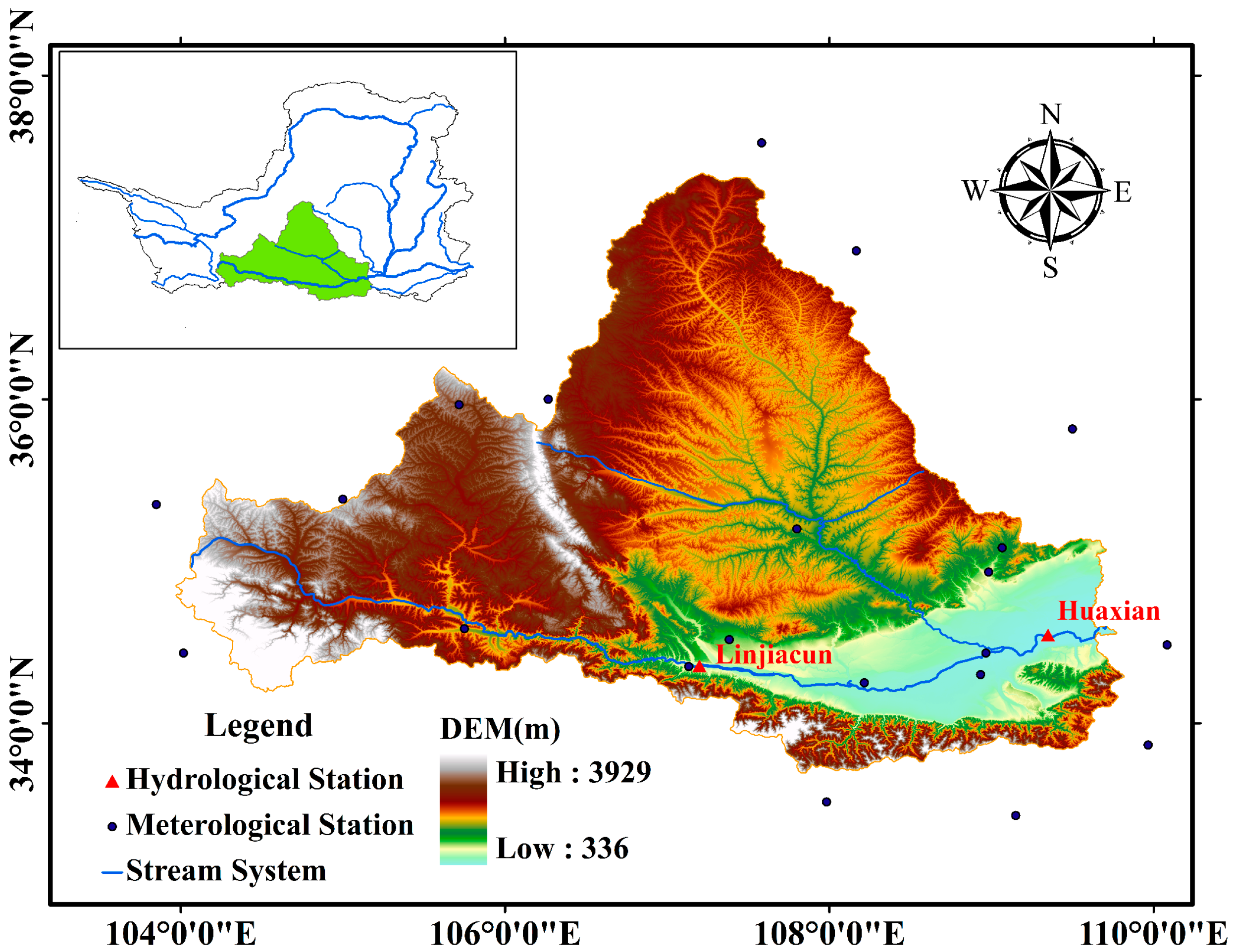
The Weihe River basin (104–107° E and 33–34° N), located in the southern part of the LP, was selected as our study area (Figure 1). The basin has a typical continental climate, and lies in the semi-humid and semi-arid transitional zone [41]. The Weihe River (hereafter WR) provides the water supply for 9300 km2 of fertile fields in the Guanzhong Plain, and more than 61% of the Shaanxi Province’s population [42]. Additionally, the start-point of the well-known Silk Road Economic Belt, Xi’an City, is situated in this basin. Mean annual precipitation varies between 400 and 600 mm, of which approximately 70% falls between June and September. Floods occur frequently after rainstorms. The largest gauged flood event at the Linjiacun station since 1960 occurred in 1966, and was 4200 m3/s.
The Weihe River basin is also one of the most serious soil loss areas on the LP. Areas suffering from severe soil loss cover approximately 65% of the total land area of this basin. It is of note that floods accelerate soil and water loss. Accelerated serious soil loss has caused severe sediment deposition in the lower reach of the WR, which poses great challenges for local flood control.
2.2. Dataset
The Linjiacun (107°03′ E, 34°22′ N) and Huaxian (109°78′ E, 34°51′ N) stations are important control stations upstream and downstream of the Weihe River basin, respectively. The locations of the two stations are displayed in Figure 1. Annual maximum flood records (1960–2012) from the two stations are utilized. The data quality was strictly controlled by the hydrology bureau of the Yellow River Conservancy Commission before the data was released. Data collected from Linjiacun and Huaxian stations can characterize the water hazard control in the Weihe River basin.
Daily precipitation data (1960–2012) are provided by the China Meteorological Data Sharing Service System (http://cdc.cma.gov.cn). The flood discharge is closely linked to the accumulated rainfall amounts before the occurrence of annual peaks [43]. Given this, the extreme precipitation event (Pr) used in present study is defined as:
where Pr denotes the accumulated rainfall from the 1st to i-th day, l is the occurrence time of peak discharge , n indicates lag time (i.e., time from peak discharge to the beginning of rainfall), means the i-th day of rainfall. The Pr1, Pr2, Pr3, Pr4 and Pr5 represent the accumulated 1-, 2-, 3-, 4- and 5-day consecutive rainfall amounts (i.e., n = 0, n = 1, n = 2, n = 3, n = 4). The Thiessen polygon method is applied to compute the areal accumulated rainfall.
To select the extreme precipitation events most closely correlated to AMF, the Kendall’s tau correlation coefficient was computed (Table 1). The Kendall’s tau is a rank-based coefficient that is robust to departures from normality. It can be found from Table 1 that Pr2 and Pr3 were most closely correlated with AMF as gauged at Xianyang and Huaxian stations, respectively.
3. Methodologies
3.1. Methodological Framework
As mentioned above, the aim of this paper is to disclose the bivariate hydrological risk and to reveal the impact of marginal distribution selection uncertainty and sampling uncertainty on hydrological risk analysis. To achieve this goal, this paper presents the following framework, as shown in Figure 2.
First, appropriate marginal distributions for AMF and Pr series were ascertained from the MEP distribution, Pearson type III distribution (P3), lognormal distribution (Logn), normal distribution (Norm) and gamma distribution (Gam). These parametric distributions are popular for characterizing the probability distributions of extreme hydrological events due to their better performance [6,44]. Second, we constructed copula models to depict the dependence structure of AMF and Pr series by joining their marginal distributions. Afterwards, the joint return periods, risk and reliability of AMF and Pr pairs were estimated for hydrological risk analysis. Last, the bivariate hydrological design events of specific joint return period were selected for hydraulic engineering design. To provide robust information for hydraulic structures design, we examined the impact of the marginal distribution selection uncertainty and sampling uncertainty on bivariate hydrological design event estimation. Here, the 6 candidate marginal distributions were combined with each other to form 36 combinations for modeling the AMF and Pr series. These combinations were utilized to explore the impact of marginal distribution uncertainty. Moreover, one Monte Carlo-based algorithm was designed to discover the impact of sampling uncertainty.
3.2. Maximum Entropy Principle Distribution (MEP)
The concept of entropy was first formulated by Shannon (1948) [45]. After that, Jaynes (1957, 1982) developed the maximum entropy principle for deriving a least-biased probability distribution when certain information is given in terms of constraints [25,46]. To date, Shannon entropy has been extensively used in the hydrological field, such as rainfall-runoff modeling, drought analysis, and flow forecasting [29,30,47,48,49].
The Shannon entropy of a probability density function (PDF) for a continuous variable can be defined as
where a and b denote the lower and upper limits of the variable X, respectively.
In order to attain the least biased probability distribution, the maximum entropy principle is performed by maximizing the entropy given by Equation (2) subject to the following constraints
where , , denotes some known functions of x; n represents the number of constraints; means the expectation of . Equation (3) states that the probability density function must satisfy the total probability theorem. Here, the can be expressed as the power of x such that
In general, different numbers of constraints would obtain different performances [50]. In light of this, the present study employs 3 and 4 constraints to build the MEP-based distributions for AMF and Pr series, respectively. The corresponding distributions are denoted as MEP-3 and MEP-4, hereafter. The impact of the number of constraints in terms of MEP distribution on bivariate design event identification will be discussed in Section 4.
To achieve the maximization of entropy, the Lagrange multiplier method is one simple and frequently used method [51]. Subject to the constraints expressed in Equations (3) and (4), the Lagrangian function L can be written as
where denotes the Lagrange multipliers.
can be attained through maximizing the function L, and therefore one differentiates L with respect to being equal to zero:
Hence, the resulting maximum entropy-based PDF of a variable X in terms of the given constraints can be written by
Inserting Equation (8) into Equations (3) and (4), respectively, we can obtain
With the use of Equation (9), the zeroth Lagrange multiplier can be written as
Substituting Equation (11) into Equation (8), can be expressed as
Here, the PDF expressed in Equation (12) can preserve the most important statistical moments. The cumulative distribution function (CDF) can be obtained through integration of Equation (12)
Based on the PDF function, the Lagrange multipliers can be estimated by minimizing the convex function, shown as
In the present study, the conjugate gradient method is employed to determine the Lagrange multipliers in Equation (14). The method is superior for solving large-scale nonlinear optimization problems. Its primary advantages are super-linear convergence, simple recurrence formula, and less calculation. Readers interested in the detailed process of determining the Lagrange multipliers through the conjugate gradient method are referred to the papers of Fan et al. (2016) [6].
3.3. Copula Function
The copula, as introduced by Sklar (1959) is a powerful tool for modeling the dependence structures of individual variables [52]. A d-dimensional copula is defined as a multivariate distribution function F [0, 1]d → [0, 1], linking standard uniform marginal distributions. Formally, the copula can be divided into two components: individual univariate distributions, and a copula function describing dependence structures between variables based on the copula and its parameter(s).
According to Sklar’s theorem, one d-dimensional multivariate distribution function F for random variables X1, X2, …, Xd with marginal distribution of F1, F2, …, Fd can be expressed as
where is the copula parameter vector and is the marginal distribution of .
In the field of hydrology, Archimedean copulas are quite popular due to their explicit functional forms. Moreover, they are superior for characterizing a wide range of dependence structures with several desirable properties. In the present study, the Clayton, Frank, and Gumbel-Hougaard copulas, which belong to the Archimedean class of copulas, were employed to evaluate the bivariate hydrological risk. The specific formula of these copulas was first reported by Nelsen (1999) [18].
3.4. Joint Return Periods, Risk and Reliability
To conduct a bivariate frequency analysis, the joint probability behaviors are defined in terms of variables X and Y, with thresholds x and y, respectively:
(1): {X>x} OR {Y>y}, (2): {X>x} AND {Y>y}
Accordingly, the joint return periods (also called primary return periods) can be written as [53,54,55]:
Here, indicates the average inter-arrival time between two successive events ( for maximum annual events).
In engineering practice, risk (hereafter, ) and reliability (hereafter, ) are another two important indices for hydraulic structure design [56]. To date, they have received widespread attention within the hydrological community [55,56,57,58,59].
Risk is defined as the probability of occurrence of at least one event exceeding the design event for the project life of n years:
where indicates the annual exceedance probability.
It should be noted that the also can be determined from the return period T ( and in this study) by substituting into Equation (18):
Reliability, which signifies the probability that a dangerous event will not occur within a project life of n years, i.e., that a system will remain in a satisfactory state within its lifetime, is defined as:
3.5. Bivariate Design Event Derived from Joint Distribution
Practical engineering design applications desire one appropriate multivariate design event or an appropriate subset of multiplets, instead of a large set of potential multiplets for the specific return period [34,60,61]. However, in a multivariate context, there exists a problem of inherent ambiguity, whereby various combinations of random variables X and Y share the same joint probability, and thus produce the same return period. Therefore, Salvadori et al. (2011) proposed a method for solving the ambiguity problem by identifying the most-likely design event [62]. The essence of the method is to identify one design event lying on critical layers for a critical level t with the largest joint probability density. The most-likely design realization can be written as:
Here, f indicates the density of , which can be expressed as
where and represent the probability density function of and , respectively; indicates the probability density function of .
is defined as:
where .
Then, the design event can be estimated by determining the largest joint probability density in the logarithmic domain on the critical layers , with the corresponding as the design realization with the joint return period T ( and in this study).
3.5.1. Uncertainty Due to the Marginal Distribution Selection
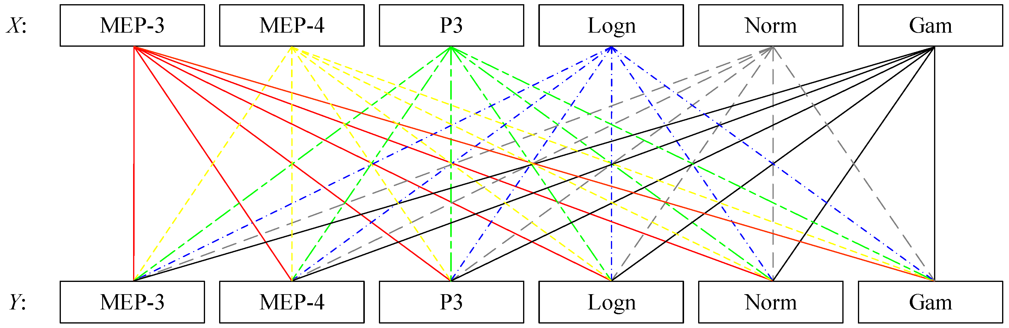
To assess the impact of marginal distribution selection uncertainty on the most-likely design event identification, we designed one experiment project by combining the 6 candidate distributions with each other to model the random variables X and Y. The 36 designed combinations are displayed in Figure 3. Then, the 36 fitted combinations are carried into Equation (21), and thus the most-likely design events for the different combinations are obtained. Through comparison among these bivariate design events, the impact of marginal distribution uncertainty is expected to be discovered.
3.5.2. Sampling Uncertainty
To determine the impact of sampling uncertainty on the most-likely design event estimation, the following Monte Carlo-based procedures were designed:
- Estimate the parameter of the copula for the observations (i.e., X and Y) as well as the parameters and of the marginal distributions for X and Y, respectively;
- Simulate bivariate samples of size on the basis of the copula parameter, and then apply the marginal backward transformations using the estimated parameters and . The simulated bivariate samples are denoted as . n is equal to the length of the observed sample. Here, B is set equal to 10,000;
- Estimate the parameters , and for the simulated sample using the same estimation method used for the observations;
- Identify the most-likely design realization for different pairs.
- Estimate the confidence intervals for at 95% confidence level by the method of highest density regions (denoted as HDR) propose by Hyndman et al. (1996) [63].
4. Results and Discussion
4.1. Marginal Distribution Selection
To construct the copula model for (AMF, Pr) in the study regions, the first step was to select appropriate marginal distributions. Table 2 lists the relevant parameters for different marginal distributions for the AMF and Pr series in the study regions.
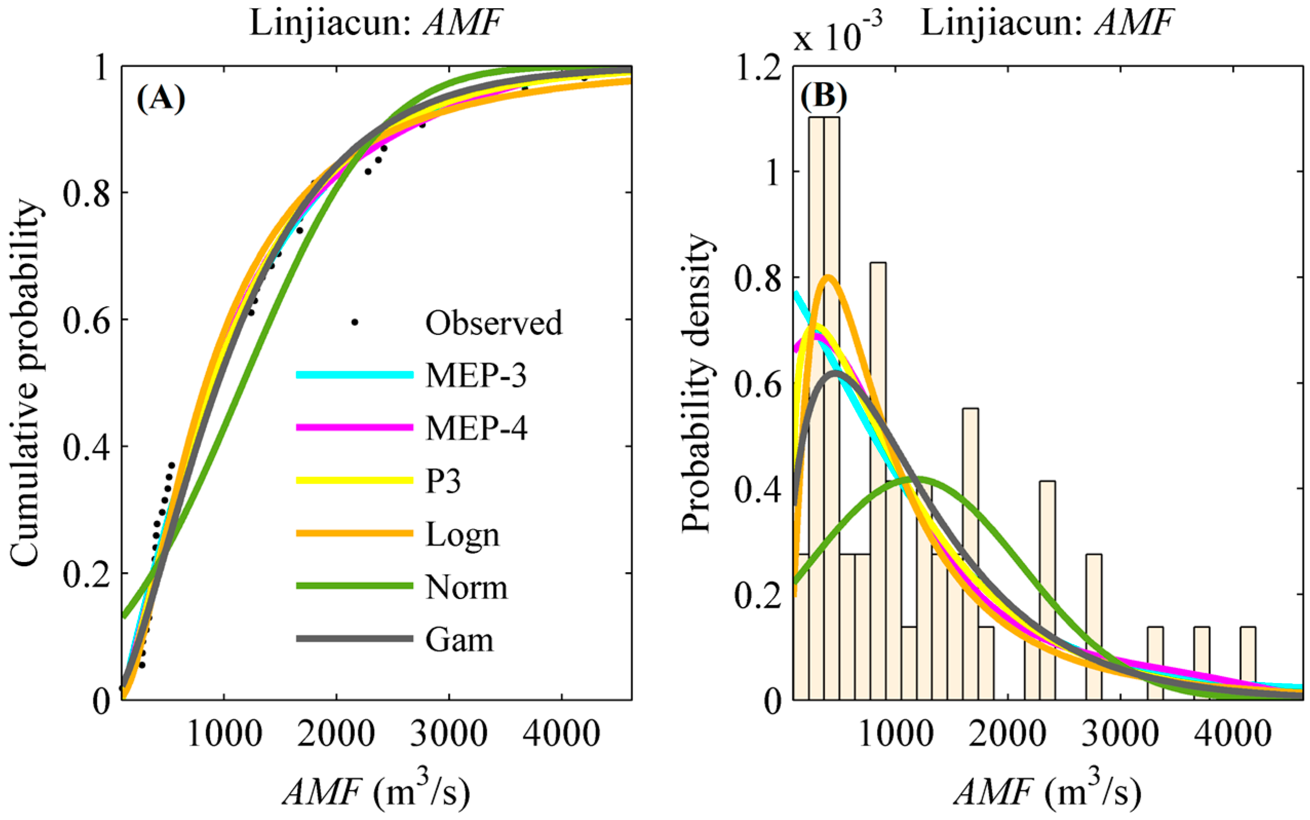
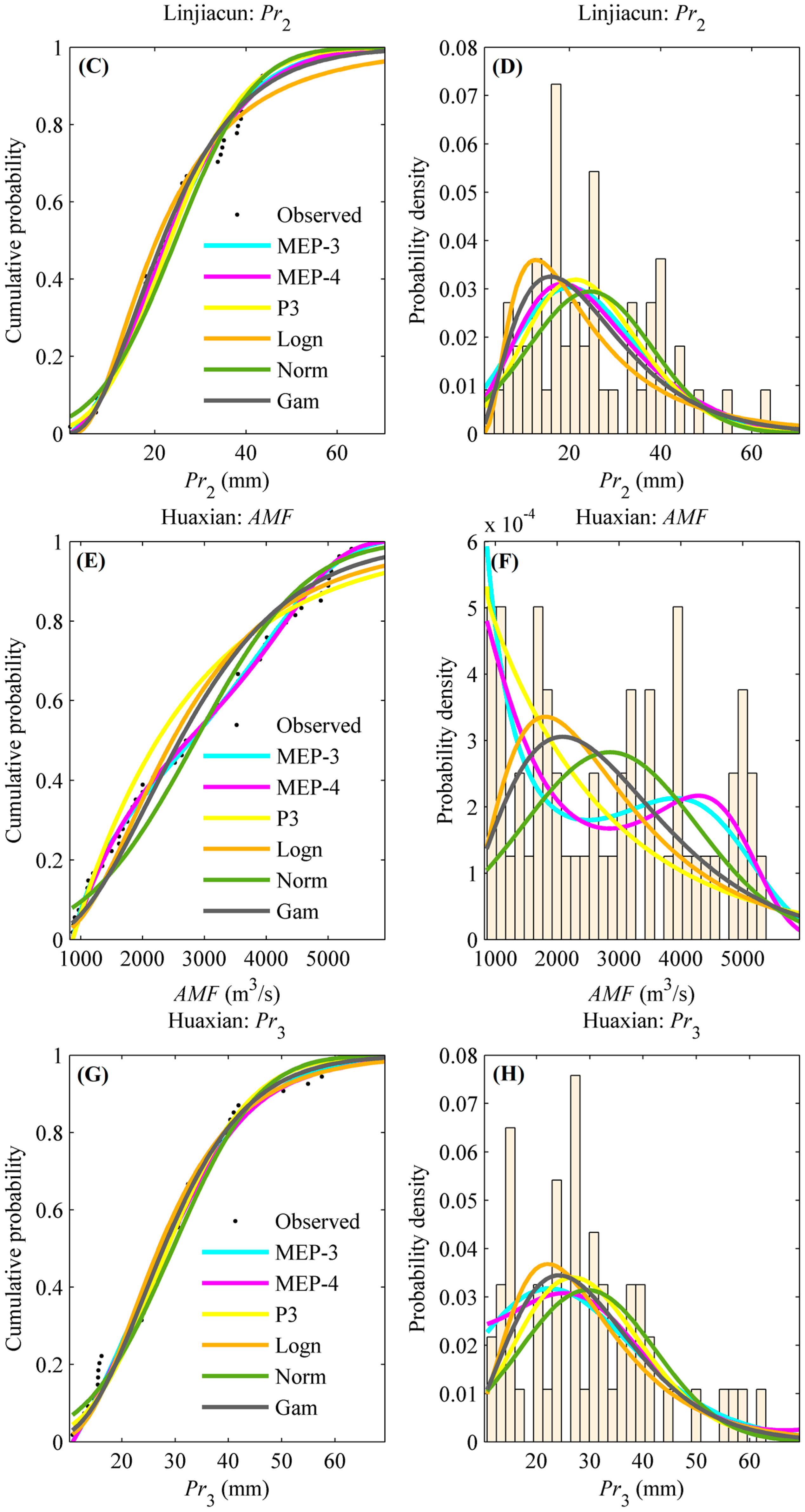
Figure 4 illustrates the distributions of the AMF and Pr series in the upper catchments of Linjiacun and Huaxian stations fitted by the MEP-3, MEP-4, P3, Logn, Norm and Gam distributions. The curves of CDF and PDF are exhibited in this figure.
It can be seen from this figure that the CDFs and PDFs exhibit variations in fitting performance between the theoretical and empirical distributions. In spite of this, it is difficult to select an appropriate fitting distribution by visual assessment. Therefore, the widely used root mean square error (RMSE) was employed to select the most appropriate model from among the candidate distribution models. The marginal distribution characterized by the minimum RMSE value was selected as the preferred model. Moreover, the goodness-of-fit test (the Kolmogorov-Smirnov (K-S) approach) was also performed to provide support in evaluating the validity of these distribution models. The K-S statistic (denoted as S) aims to quantify the largest vertical difference between the empirical and estimated distributions [64]. The p-value of the K-S statistic was obtained by using Miller’s approximation. A value of p bigger than 0.05 indicates that the candidate distribution can appropriately fit random variables at the 5% significance level.
The RMSE values and K-S test results are presented in Table 3. It can be seen from Table 3 that the p values were much higher than the significance level 0.05, signifying that these candidate distributions are suitable for fitting the distributions of the AMF and Pr series. The RMSE values listed in Table 3 indicate that the MEP-4 distribution could be selected as the appropriate distribution for fitting the AMF and Pr series in the upper catchment of Linjiacun station, while MEP-3 and MEP-4 performed best among the candidates for fitting the AMF and Pr series, respectively, in the upper catchment of Huaxian station.
A closer look at the fitting performance of these distributions for the AMF series at Linjiacun station, as presented in Figure 4 and Table 3, indicates that the fitting performance among the different distributions were similar, except for the Norm distribution. The RMSE values were 0.0303, 0.0296, 0.0309, 0.0366 and 0.0405 for the MEP-3, MEP-4, P3, Logn and Gam distributions, respectively, and 0.0823 for the Norm distribution. In terms of the Pr2 series in the upper catchment of Linjiacun station, the Norm distribution had the worst performance of all the candidates.
As for the AMF series at the Huaxian station, the MEP-3 distribution outperformed other candidates (RMSE = 0.0195). The RMSE values for MEP-4, P3, Logn, Norm and Gam distributions ranged from 0.0202 to 0.0686. As shown in Figure 4, the histogram of the AMF series at Huaxian station has two peaks. MEP distribution can deal with multiple modes, while conventional models fail to fit a distribution with more than one mode. This is the reason that the conventional distributions show poor performance when fitting the AMF series at Huaxian station, while for the Pr3 series in the upper catchment of Huaxian station, a comparison of RMSE values among the candidates indicates that the MEP-4 distribution (RMSE = 0.0267) performed better than other candidates (ranging from 0.0299 to 0.0390).
In light of the above findings, it can be concluded that MEP-related functions provide a better alternative than other conventional distributions for modeling the AMF and Pr series. Specifically, due to the PDF of the variables consisting of a single mode, the fitting performances of MEP-related distributions were similar to certain conventional distributions. The fitting performance of distributions for the AMF and Pr2 series at Linjiacun station and the Pr3 series at Huaxian station are able to demonstrate this inference. Moreover, it also can be inferred that the MEP-related distributions outperform the conventional distributions, particularly when modeling the distribution of random variables exhibiting multiple modes in the histogram, such as the AMF series at Huaxian station. These findings are similar to those obtained in Zhou et al. (2010) and Liu and Chang (2011) when fitting the distribution of wind speed data [65,66].
Additionally, we should also note that there exist some disadvantages to the MEP distribution; for example, the CDF of MEP-related distributions cannot be expressed in a closed form, parameter estimation is computationally expensive, and the mathematical expression of MEP-related distributions is more complex to develop as a computer program [6,66].
4.2. Copula Function Construction
Once the marginal distribution is chosen, the next step is to estimate the parameters of the copula and select an appropriate copula function from among the Clayton, Frank and Gumbel copulas. The parameters of the copulas are estimated using the maximum pseudo-likelihood method. The constructed MEP-related distributions are used to quantify the marginal probabilities of the AMF and Pr series. The estimated parameters of these candidate copulas are listed in Table 4.
To select the suitable copulas, the Cramér–von Mises test was used to test goodness-of-fit based on the empirical copula. Table 4 lists the goodness-of-fit statistics Sn corresponding to the Cramér–von Mises criteria, and their associated p-value based on N = 10,000 parametric bootstrap samples. A larger value of Sn indicates greater distance between the estimated and the empirical copulas. p-value > 0.05 means the estimated copula can be accepted at the 5% level. Results displayed in Table 4 illustrate that these candidate copulas are all acceptable for fitting the dependence structures between AMF and Pr in each region at a 5% significance level.
Further, the corrected Akaike information criterion (AICc) indicator is employed to select the copula with the highest fitting performance (shown in Table 4). The AICc indicator is much stricter than classical AIC, particularly when the size of the hydrological observations is limited [67]. The copula distribution characterized by the minimum AICc value was selected as the preferred model. It can be seen from Table 4 that the Gumbel and Frank copulas should be chosen to model the joint distribution of AMF and Pr series in the upper catchments of Linjiacun and Huaxian stations, respectively. For simplicity, the bivariate model constructed by integrating the MEP distributions into the copula is denoted as MEP-copula.
4.3. Bivariate Return Period, Risk and Reliability Analysis Based on the MEP-Copula
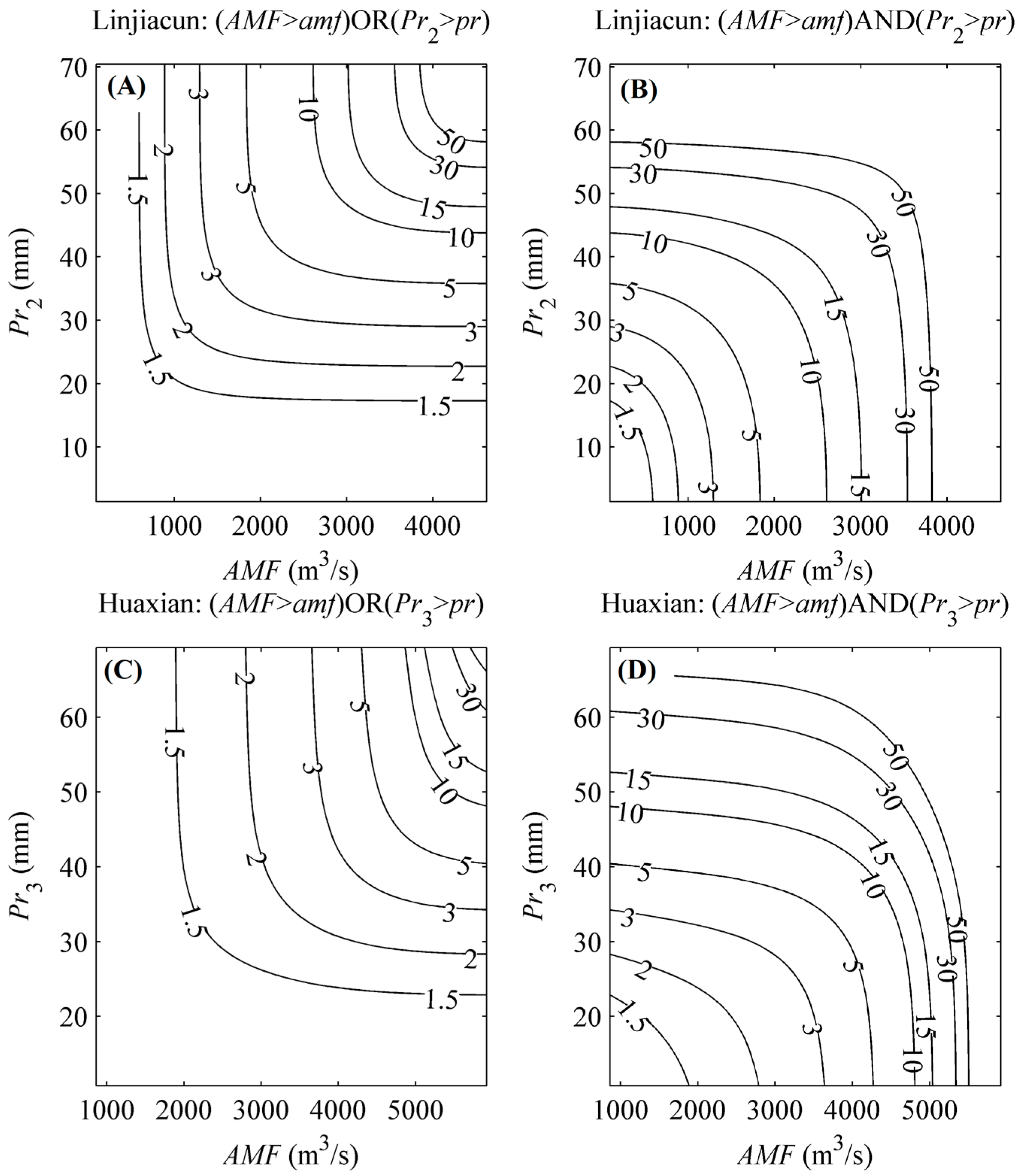
Exploring the concurrence probabilities of various combinations of AMF and Pr is of critical importance for practical flood control and disaster mitigation. As expressed as Equations (16) and (17), the bivariate return periods are estimated based on the constructed MEP-copula models. Figure 5 displays the bivariate joint return periods of “AND” and “OR” cases for various (AMF, Pr) pairs. It can be seen from Figure 5 that the joint return period level of the “AND” case is concave, while that for the “OR” case is convex. Generally, the joint return period of the “AND” case is lower than that of the “OR” case. For instance, if both the AMF and Pr observed in the upper catchment of Linjiacun station are in the 20-year return period, the “AND” joint return period of the (AMF, Pr) pair is 42.23 years, while the “OR” joint return period is 13.10 years. Additionally, in practical terms, water resource managers and policy-makers can identify the return periods for various (AMF, Pr) pairs of observations or forecasts through Figure 5.
In engineering design of hydrological infrastructures, risk can be defined as the likelihood of experiencing at least one event exceeding the design event over the design life (denoted as n) of the hydraulic structure [6]. Furthermore, reliability over the project life is commonly chosen to describe the probability that the hydraulic structure will remain in a satisfactory state within its project life [60]. In the present study, the “AND” joint return period case is applied to define the bivariate risk and reliability through Equations (18)–(20). Here, the service time of a river levee is assumed to be 10 years, i.e., n = 10.
Figure 6 exhibits the bivariate risk and reliability under different designed AMF and Pr combinations in the two regions. It can be found from Figure 6 that the risk value would decrease as the designed AMF or Pr increased, which is contrary to the reliability value. In other words, higher values of the designed AMF or Pr for the hydraulic structure indicate a smaller probability for the occurrence of an undesirable flood event within a project life of n years, and a higher probability that the hydraulic structure will remain in a satisfactory state.
The implication for the bivariate risk and reliability of (AMF, Pr) pairs is to provide decision support for hydraulic structures and practical flood control. Decision-makers can attain the corresponding risk and reliability under various AMF and Pr scenarios as the design events for the hydraulic structure. For example, if the design event for a river levee in the downstream area of Huaxian station is set to (5000 m3/s, 39.02 mm), the corresponding risk (reliability) that that event (AMF > 5000 m3/s) AND (Pr3 > 39.02 mm) will occur (not occur) during the river levee life of 10 years is 0.3331 (0.6669). Clearly, if decision-makers tend to decrease the risk or increase the reliability, the values of (AMF, Pr) pair should be improved.
4.4. Bivariate Design Event Identification
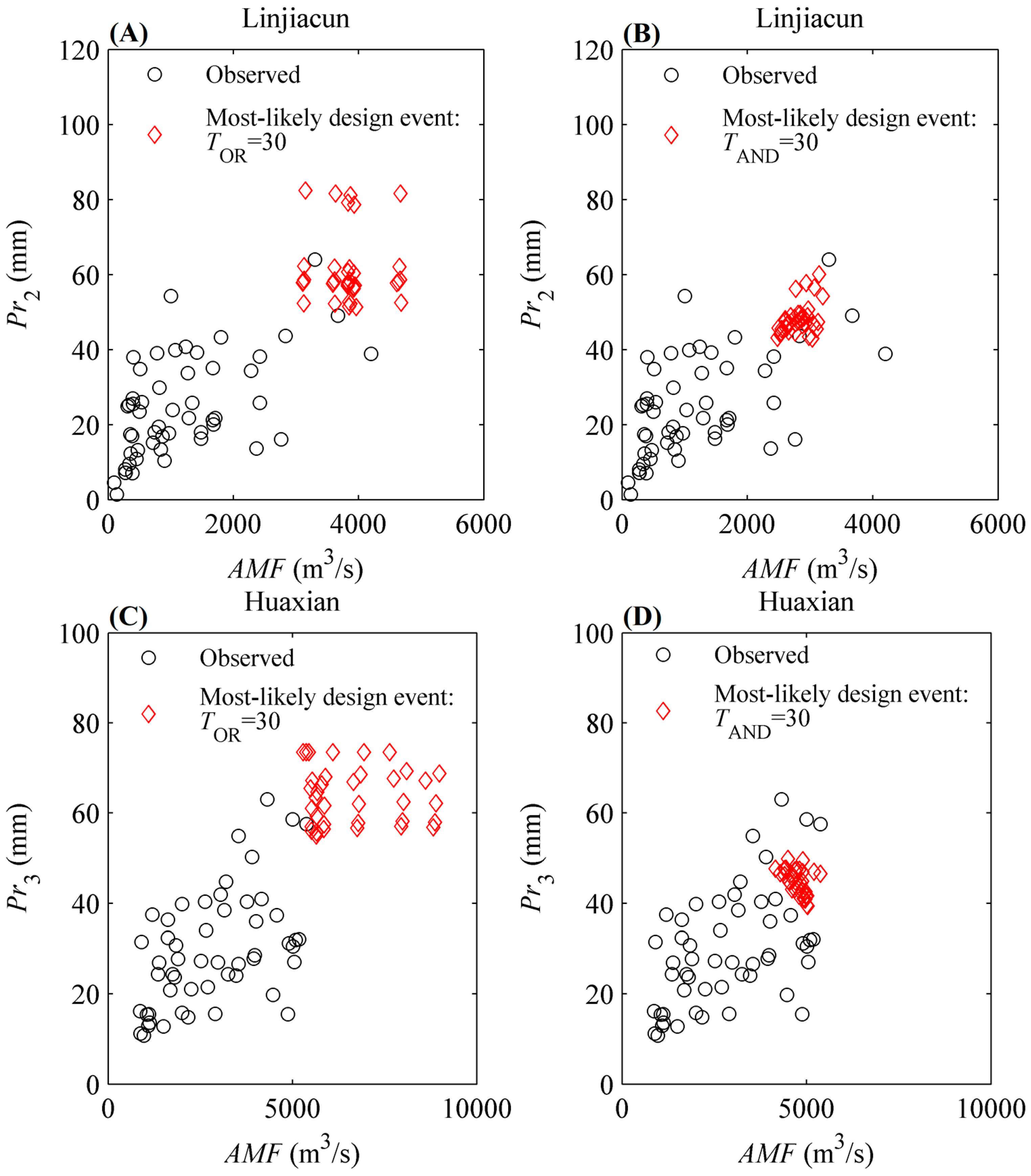
In practical hydrological facility design, unique design realization on the isoline is obligatory and crucial. As is widely known, higher values of design event for hydraulic structures lead to poor economy, while lower values have a negative impact on the safety of flood control. However, as displayed in Section 4.3, for the specified return period, risk or reliability, there is a large set of potential (AMF, Pr) events. Therefore, appropriate methods for identifying the unique design realization from the return level curve is of great necessity. In the present study, the most-likely design event method is utilized, as described previously in the literature [23,60,62]. The constructed MEP-copula is applied to estimate the most-likely design event. Table 5 lists the most-likely design events determined given TOR = TAND = 30 years using Equation (21) in the study regions. It can be seen from Table 5 that the most-likely design events for the upper catchments of Linjiacun and Huaxian stations are (3825.82 m3/s, 56.95 mm) and (5369.10 m3/s, 73.46 mm) given TOR = 30 years, respectively, while given TAND = 30 years, they are (3052.79 m3/s, 46.76 mm) and (5017.84 m3/s, 41.64 mm), respectively.
4.4.1. Uncertainty Due to Marginal Distribution Selection
In order to explore the impact of the uncertainty of marginal distribution selection on design event estimation, an extended experiment combining different marginal distributions was conducted. These selected marginal distributions all passed the goodness-of-fit test at the 5% significance level. The copula functions that modeled the joint distributions of (AMF, Pr) pairs in the upper catchments of the Linjiacun and Huaxian stations were the Gumbel and Frank copulas, respectively. Figure 3 exhibits the analyzed combinations of different marginal distributions. Given TOR = TAND = 30 years, and the estimated most-likely design events under different combinations of marginal distributions are shown in Figure 7 and Table 5.
It can be seen from Figure 7 and Table 5 that there is a remarkable difference among these design events for the “OR” case under different combinations of marginal distributions. Among these estimated (AMF, Pr) pairs, the AMF value ranges from 3108.07 m3/s to 4681.88 m3/s in the upper catchment of Linjiacun station, while the Pr value ranges from 51.29 mm to 82.35 mm. The corresponding cumulative probability for the AMF series varies between 0.97 and 0.98, while that for the Pr series ranges between 0.97 and 0.99.
As for the “AND” case, it can be seen from Figure 7 that the difference among these design events estimated under different combinations of marginal distributions is smaller than that for the “OR” case. Take the upper catchment of Linjiacun station, for example; among these estimated (AMF, Pr) pairs, the AMF value ranges from 2481.91 m3/s to 3204.83 m3/s in the “AND” case, while the Pr value ranges from 42.96 mm to 60.07 mm. The corresponding cumulative probability of AMF values varies between 0.89 and 0.96, while that for the Pr value varies between 0.84 and 0.95.
To further explore the reasons for the difference among design events for the “OR” and “AND” cases, we exemplarily display part of CDF curves for AMF and Pr series for the upper catchment of Linjiacun station in Figure 8. Figure 8 illustrates that the difference of the fitting performance of different marginal distributions increases with the values of the variables. In other words, the smaller the value of AMF/Pr or the cumulative probability of AMF/Pr is, the smaller the difference in fitting performance among these distributions is. When TOR = TAND = 30 years, the corresponding cumulative probability of AMF in the “OR” case ([0.97–0.98]) is larger than that in the “AND” case ([0.89–0.96]), which is the same as that of Pr. Therefore, the difference among design events in the “AND” case is smaller than that in the “OR” case. This finding is consistent with that of Dung et al. (2015) [35].
4.4.2. Uncertainty Due to the Limited Size of Hydrological Records
In order to uncover the impact of sampling uncertainty on the most-likely design event estimation, the designed Monte Carlo algorithm in Section 3.5.2 was utilized. Here, the AMF and Pr series were modeled by the MEP-related distributions. The Gumbel and Frank copulas were applied to describe the joint distribution of (AMF, Pr) pairs in the upper catchments of Linjiacun and Huaxian stations, respectively.
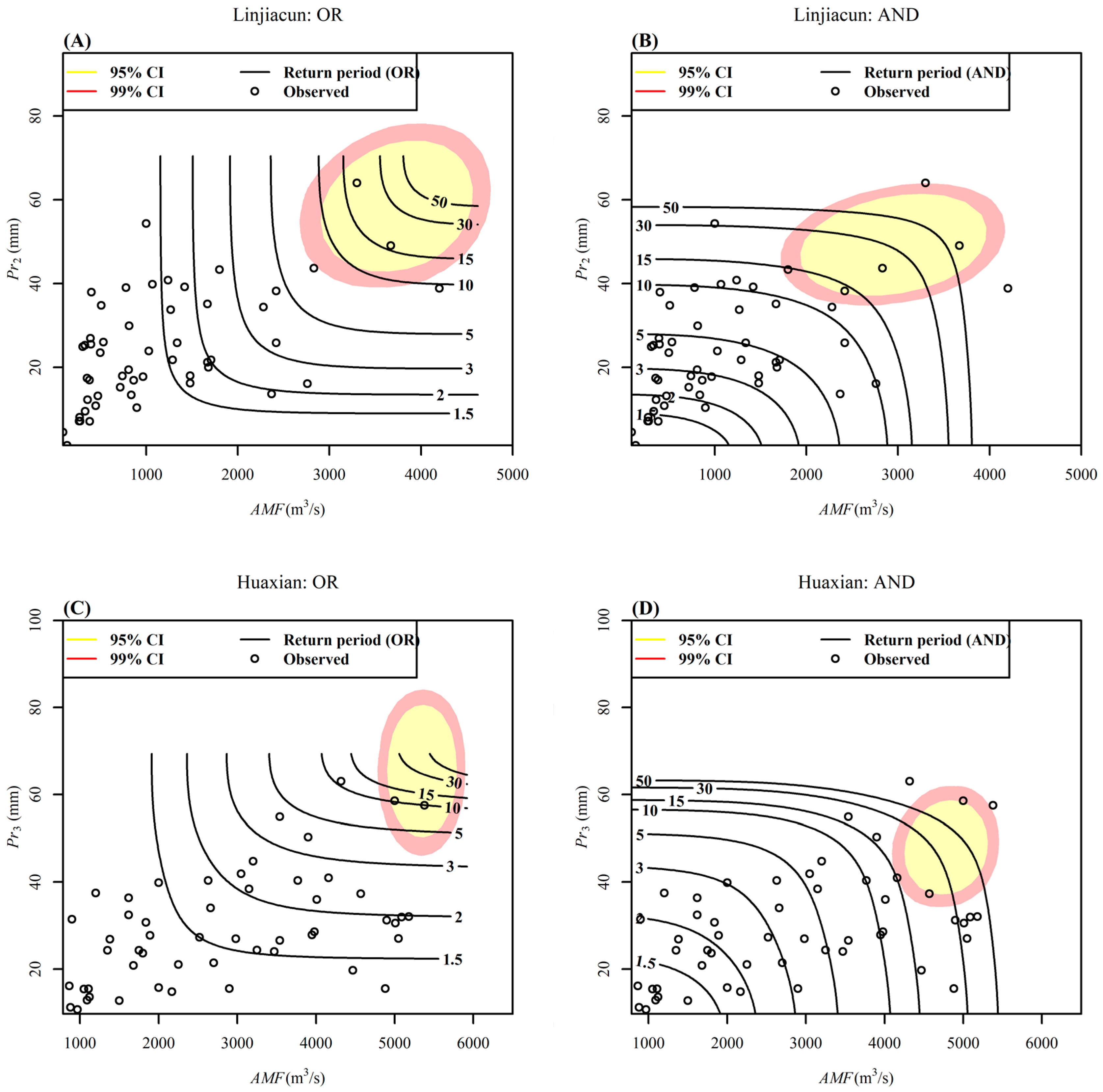
Moreover, Figure 9 clearly shows the confidence regions of the most-likely design events with TOR = TAND = 30 years using the HDR method. The highest density regions (95% and 99%) are exhibited in a two-dimensional plane (AMF-Pr) that correspond to a return period of 30 years. It can be seen from Figure 9 that the confidence regions of the most-likely design events for TOR = TAND = 30 years are very large in the study regions. The 95% confidence region for the most-likely design events in terms of AMF and Pr with a return period of 30 years could range between values for AMF and Pr with return periods of 10 and 50 years, at least. Take the upper catchment of Linjiacun station, for example; in the 95% region for TOR = 30 years, the AMF could assume values with a univariate return period from 10 to 50 years. Large uncertainties due to sampling uncertainty can also be found in the works of [34,35,68,69], i.e., the return periods of the most-likely design events overlap. These large uncertainties present a significant challenge for reservoir design, flood risk, etc., particularly for Guanzhong plain, as one of the most important Chinese agricultural production regions, and Xi’an city, as one of the four major ancient capitals of civilization, which lie in the floodplain between Linjiacun and Huaxian stations. Uncertainty of copula-based frequency analysis for the study regions should arouse critical concern, particularly when constituting policy for flood control and hazard reduction.
5. Summary and Conclusions
In this study, one general framework, aiming to analyze bivariate hydrological risk through a coupled maximum entropy-copula method and to reveal the impact of marginal distribution selection uncertainty and sampling uncertainty on hydrological risk analysis, is proposed.
The framework excels previous studies in applying the maximum entropy principle-based marginal distribution for modeling random variables and accounting for the impact of different uncertainty sources on hydrological risk analysis. The joint return periods, risk reliability, and bivariate design events are derived based on the coupled maximum entropy-copula method. For the purpose of practical engineering design applications, the so-called most-likely design event is identified to characterize the bivariate design event. To reveal the impact of marginal distribution selection uncertainty and sampling uncertainty on the bivariate design event identification, we designed a corresponding experiment project and specific Monte Carlo-based algorithm to achieve the two goals, respectively. Here, to elucidate the impact of marginal distribution uncertainty on the bivariate design event identification, 6 candidate distributions were combined with each other to produce 36 combinations for fitting univariate flood and extreme precipitation series. Then, these combinations concerning the marginal distributions of flood and extreme precipitation events were utilized to derive the bivariate design event. For the second goal, the Monte Carlo-based algorithm was designed to disclose the impact of sampling uncertainty on the bivariate design event identification.
Two sub-catchments of Loess Plateau, which were typical eco-environmentally vulnerable regions, were selected as the study regions. The primary conclusions are drawn as follows:
- (1)
- The maximum entropy principle (MEP)-based distributions outperform the conventional distributions (i.e., P3, Logn, Norm and Gam at least in this study) in quantifying the probability of flood and extreme precipitation events. Results of this study indicate the better performance of MEP distribution, suggesting that it could be an attractive alternative for quantifying the marginal probability of random variables.
- (2)
- The Gumbel and Frank copulas were suitable dependence models for quantifying the joint probabilities of flood and extreme precipitation events in the upper catchments of Linjiacun and Huaxian stations, respectively.
- (3)
- The bivariate return periods, risk and reliability of flood and extreme precipitation events for the two study regions were calculated based on the coupled maximum entropy-copula models, which were expected to provide practical support for the local flood control and disaster mitigation.
- (4)
- The bivariate design realizations were estimated for the study regions. Comprehensive uncertainty analysis revealed that the fitting performance of univariate distribution is closely related to the bivariate design event identification. If the difference of the fitting performance between two marginal distributions is small, values of the bivariate design events are similar, and vice versa. Therefore, advanced univariate distribution is critical for the bivariate design event selection.
Most importantly, the uncertainty related to the limited sample size is considerable, and should arouse critical attention. The bivariate design events of a specific return period exhibit significant variation. In other words, the return periods of the most-likely design events overlap. The 95% confidence regions of bivariate design events for flood and extreme precipitation with a return period of 30 years could reach between the values for flood and extreme precipitation with return periods of 10 and 50 years. The overlap phenomenon poses great challenges for practical engineering design applications, flood control, and so on. To enable a more reliable estimation of the design realization, increasing the information content by expanding the temporal, spatial or causal data is desirable, as proposed by Merz and Blöschl (2008) [70].
Acknowledgments
This work was supported by the National Key Research and Development Program of China (2016YFC0400906), National Natural Science Foundation of China (51679187, 51679189), National Key R & D Program of China (2017YFC0405900), Innovation Fund for doctoral dissertation of Xi’an University of Technology (310-252071606, 310-252071605), and the China Scholarship Council (CSC). Sincere gratitude is extended to the editor and the anonymous reviewers for their professional comments and corrections.
Author Contributions
Jianxia Chang and Aijun Guo designed the experiment; Aijun Guo performed the experiment and wrote the draft of the paper; Jianxia Chang, Yimin Wang and Qiang Huang revised the paper; Zhihui Guo drew figures. All authors have read and approved the final manuscript.
Conflicts of Interest
The authors declare no conflict of interest.
References
- Nie, C.; Li, H.; Yang, L.; Wu, S.; Liu, Y.; Liao, Y. Spatial and temporal changes in flooding and the affecting factors in China. Nat. Hazards 2012, 61, 425–439. [Google Scholar] [CrossRef]
- Merz, B.; Nguyen, V.D.; Vorogushyn, S. Temporal clustering of floods in Germany: Do flood-rich and flood-poor periods exist? J. Hydrol. 2016, 541B, 824–883. [Google Scholar] [CrossRef]
- Swierczynski, T.; Ionita, M.; Pino González, D. Using archives of past floods to estimate future flood hazards. EOS Trans. 2017, 98. [Google Scholar] [CrossRef]
- UNISDR. The Human Cost of Weather-Related Disasters 1995–2015. 2015. Available online: http://www.unisdr.org/archive/46793 (accessed on 11 November 2017).
- Svetlana, D.; Radovan, D.; Ján, D. The economic impact of floods and their importance in different regions of the world with emphasis on Europe. Procedia Econ. Financ. 2015, 34, 649–655. [Google Scholar] [CrossRef]
- Fan, Y.R.; Huang, W.W.; Huang, G.H.; Huang, K.; Li, Y.P.; Kong, X.M. Bivariate hydrologic risk analysis based on a coupled entropy-copula method for the Xiangxi river in the three Gorges Reservoir area, China. Theor. Appl. Climatol. 2016, 125, 381–397. [Google Scholar] [CrossRef]
- Li, F.; Zheng, Q. Probabilistic modelling of flood events using the entropy copula. Adv. Water Res. 2016, 97, 233–240. [Google Scholar] [CrossRef]
- Blöschl, G.; Gaál, L.; Hall, J.; Kiss, A.; Komma, J.; Nester, T.; Parajka, J.; Perdigão, R.A.P.; Plavcová, L.; Rogger, M.; et al. Increasing river floods: Fiction or reality? WIREs Water 2015, 2, 329–344. [Google Scholar] [CrossRef] [PubMed]
- Machado, M.J.; Botero, B.A.; López, J.; Francés, F.; Díez-Herrero, A.; Benito, G. Flood frequency analysis of historical flood data under stationary and non-stationary modelling. Hydrol. Earth Syst. Sci. Discuss. 2015, 12, 525–568. [Google Scholar] [CrossRef]
- Kiem, A.S.; Verdon-Kidd, D.C. The importance of understanding drivers of hydroclimatic variability for robust flood risk planning in the coastal zone. Australas. J. Water Res. 2013, 17, 126–134. [Google Scholar] [CrossRef]
- Madsen, H.; Lawrence, D.; Lang, M.; Martinkova, M.; Kjeldsen, T.R. Review of trend analysis and climate change projections of extreme precipitation and floods in Europe. J. Hydrol. 2014, 519, 3634–3650. [Google Scholar] [CrossRef] [Green Version]
- Liu, D.; Wang, D.; Singh, V.P.; Wang, Y.; Wu, J.; Wang, L.; Zou, X.; Chen, Y.; Chen, X. Optimal moment determination in POME-copula based hydrometeorological dependence modelling. Adv. Water Res. 2017, 105, 39–50. [Google Scholar] [CrossRef]
- Zhang, L.; Singh, V.P. Bivariate flood frequency analysis using the copula method. J. Hydrol. Eng. 2006, 11, 150–164. [Google Scholar] [CrossRef]
- Karmakar, S.; Simonovic, S.P. Bivariate flood frequency analysis. Part 2: A copula-based approach with mixed marginal distributions. J. Flood Risk Manag. 2009, 2, 32–44. [Google Scholar] [CrossRef]
- Ozga-Zielinski, B.; Ciupak, M.; Adamowski, J.; Khalil, B.; Malard, J. Snow-melt flood frequency analysis by means of copula based 2D probability distributions for the Narew river in Poland. J. Hydrol. Reg. Stud. 2016, 6, 26–51. [Google Scholar] [CrossRef]
- Chen, L.; Singh, V.P.; Guo, S.; Mishra, A.K.; Guo, J. Drought analysis using copulas. J. Hydrol. Eng. 2013, 18, 797–808. [Google Scholar] [CrossRef]
- She, D.; Mishra, A.K.; Xia, J.; Zhang, L.; Zhang, X. Wet and dry spell analysis using copulas. Int. J. Climatol. 2016, 36, 476–491. [Google Scholar] [CrossRef]
- Nelsen, R.B. An Introduction to Copulas, 2nd ed.; Springer: Berlin, Germany, 2006. [Google Scholar]
- Khedun, C.P.; Mishra, A.K.; Singh, V.P.; Giardino, J.R. A copula-based precipitation forecasting model: Investigating the interdecadal modulation of ENSO’s impacts on monthly precipitation. Water Resour. Res. 2014, 50, 580–600. [Google Scholar] [CrossRef]
- Fan, Y.R.; Huang, G.H.; Baetz, B.W.; Li, Y.P.; Huang, K. Development of copula-based particle filter (CopPF) approach for hydrologic data assimilation under consideration of parameter interdependence. Water Resour. Res. 2017, 53, 4850–4875. [Google Scholar] [CrossRef]
- Laux, P.; Vogl, S.; Qiu, W.; Knoche, H.R.; Kunstmann, H. Copula-based statistical refinement of precipitation in RCM simulations over complex terrain. Hydrol. Earth Syst. Sci. 2011, 15, 2401–2419. [Google Scholar] [CrossRef] [Green Version]
- Bobee, B.; Cavidas, G.; Ashkar, F.; Bernier, J.; Rasmussen, P. Towards a systematic approach to comparing distributions used in flood frequency analysis. J. Hydrol. 1993, 142, 121–136. [Google Scholar] [CrossRef]
- Volpi, E.; Fiori, A. Design event selection in bivariate hydrological frequency analysis. Hydrol. Sci. J. 2012, 57, 1506–1515. [Google Scholar] [CrossRef]
- Zhang, L.; Singh, V.P. Bivariate rainfall and runoff analysis using entropy and copula theories. Entropy 2012, 14, 1784–1812. [Google Scholar] [CrossRef]
- Jaynes, E.T. Information theory and statistical mechanics. Phys. Rev. 1957, 106, 620. [Google Scholar] [CrossRef]
- AghaKouchak, A. Entropy—Copula in hydrology and climatology. J. Hydrometeorol. 2014, 15, 2176–2189. [Google Scholar] [CrossRef]
- Zhao, N.; Lin, W.T. A copula entropy approach to correlation measurement at the country level. Appl. Math. Comput. 2011, 218, 628–642. [Google Scholar] [CrossRef]
- Dong, S.; Wang, N.; Liu, W.; Soares, C.G. Bivariate maximum entropy distribution of significant wave height and peak period. Ocean Eng. 2013, 59, 86–99. [Google Scholar] [CrossRef]
- Chen, L.; Singh, V.P.; Xiong, F. An Entropy-based generalized gamma distribution for flood frequency analysis. Entropy 2017, 19, 239. [Google Scholar] [CrossRef]
- Hao, Z.; Singh, V.P. Integrating entropy and copula theories for hydrologic modeling and analysis. Entropy 2015, 17, 2253–2280. [Google Scholar] [CrossRef]
- Mishra, A.K.; Özger, M.; Singh, V.P. An entropy-based investigation into the variability of precipitation. J. Hydrol. 2009, 370, 139–154. [Google Scholar] [CrossRef]
- Rajsekhar, D.; Mishra, A.K.; Singh, V.P. Regionalization of drought characteristics using an entropy approach. J. Hydrol. Eng. 2013, 18, 870–887. [Google Scholar] [CrossRef]
- Michailidi, E.M.; Bacchi, B. Dealing with uncertainty in the probability of overtopping of a flood mitigation dam. Hydrol. Earth Syst. Sci. 2017, 21, 2497–2507. [Google Scholar] [CrossRef]
- Serinaldi, F. An uncertain journey around the tails of multivariate hydrological distributions. Water Resour. Res. 2013, 49, 6527–6547. [Google Scholar] [CrossRef]
- Dung, N.V.; Merz, B.; Bardossy, A.; Apel, H. Handling uncertainty in bivariate quantile estimation—An application to flood hazard analysis in the Mekong Delta. J. Hydrol. 2015, 527, 704–717. [Google Scholar] [CrossRef]
- Serinaldi, F.; Kilsby, C.G. Stationarity is undead: Uncertainty dominates the distribution of extremes. Adv. Water Resour. 2015, 77, 17–36. [Google Scholar] [CrossRef]
- Zhang, X.; Zhang, L.; Zhao, J.; Rustomji, P.; Hairsine, P. Responses of streamflow to changes in climate and land use/cover in the Loess Plateau, China. Water Resour. Res. 2008, 44. [Google Scholar] [CrossRef]
- Shi, H.; Shao, M. Soil and water loss from the Loess Plateau in China. J. Arid Environ. 2000, 45, 9–20. [Google Scholar] [CrossRef]
- Du, T.; Xiong, L.; Xu, C.Y.; Gippel, C.J.; Guo, S.; Liu, P. Return period and risk analysis of nonstationary low-flow series under climate change. J. Hydrol. 2015, 527, 234–250. [Google Scholar] [CrossRef]
- Ma, M.; Song, S.; Ren, L.; Jiang, S.; Song, J. Multivariate drought characteristics using trivariate Gaussian and student copula. Hydrol. Process. 2013, 27, 1175–1190. [Google Scholar] [CrossRef]
- Peng, H.; Jia, Y.W.; Tague, C.; Slaughter, P. An eco-hydrological model-based assessment of the impacts of soil and water conservation management in the Jinghe river basin, China. Water 2015, 7, 6301–6320. [Google Scholar] [CrossRef]
- Guo, A.; Chang, J.; Huang, Q.; Wang, Y.; Liu, D.; Li, Y.; Tian, T. Hybrid method for assessing the multi-scale periodic characteristics of the precipitation—Runoff relationship: A case study in the Weihe river basin, China. J. Water Clim. Chang. 2017, 8, 62–77. [Google Scholar] [CrossRef]
- Teegavarapu, R.S.V. Floods in Changing Climate; Cambridge University Press: New York, NY, USA, 2012. [Google Scholar]
- Kamal, V.; Mukherjee, S.; Singh, P.; Sen, R.; Vishwakarma, C.A.; Sajadi, P.; Asthana, H.; Rena, V. Flood frequency analysis of Ganga river at Haridwar and Garhmukteshwar. Appl. Water Sci. 2017, 7, 1979–1986. [Google Scholar] [CrossRef]
- Shannon, C.E. A mathematical theory of communications. Bell Syst. Tech. J. 1948, 27, 379–423. [Google Scholar] [CrossRef]
- Jaynes, E.T. On the rationale of maximum-entropy methods. Proc. IEEE 1982, 70, 939–952. [Google Scholar] [CrossRef]
- Cui, H.; Singh, V.P. Maximum entropy spectral analysis for streamflow forecasting. Phys. A Stat. Mech. Appl. 2016, 442, 91–99. [Google Scholar] [CrossRef]
- Li, C.; Singh, V.P.; Mishra, A.K. Entropy theory-based criterion for hydrometric network evaluation and design: Maximum information minimum redundancy. Water Resour. Res. 2012, 48. [Google Scholar] [CrossRef]
- Mishra, A.K.; Ines, A.V.M.; Singh, V.P.; Hansen, J.W. Extraction of information content from stochastic disaggregation and bias corrected downscaled precipitation variables for crop simulation. Stoch. Environ. Res. Risk Access. 2013, 27, 449–457. [Google Scholar] [CrossRef]
- Singh, V.P. Hydrologic synthesis using entropy theory. J. Hydrol. Eng. 2011, 16, 421–433. [Google Scholar] [CrossRef]
- Singh, V.P.; Rajagopal, A.K. A new method of parameter estimation for hydrologic frequency analysis. Hydrol. Sci. Technol. 1987, 2, 33–40. [Google Scholar]
- Sklar, A. Functions de Repartition à n Dimensions et Luers Marges. Publ. Inst. Stat. Univ. Paris 1959, 8, 229–231. [Google Scholar]
- Salvadori, G.; De Michele, C.; Kottegoda, N.T.; Rosso, R. Extremes in Nature: An Approach Using Copulas; Springer: New York, NY, USA, 2007. [Google Scholar]
- Vandenberghe, S.; Verhoest, N.E.C.; Onof, C.; De Baets, B. A comparative copula-based bivariate frequency analysis of observed and simulated storm events: A case study on Bartlett-Lewis modeled rainfall. Water Resour. Res. 2011, 47. [Google Scholar] [CrossRef]
- Fan, Y.R.; Huang, W.; Huang, G.H.; Li, Y.P.; Huang, K. Hydrologic risk analysis in the Yangtze river basin through coupling Gaussian mixtures into copulas. Adv. Water Resour. 2016, 88, 170–185. [Google Scholar] [CrossRef]
- Salas, J.D.; Obeysekera, J. Revisiting the concepts of return period and risk for nonstationary hydrologic extreme events. J. Hydrol. Eng. 2013, 19, 554–568. [Google Scholar] [CrossRef]
- Mood, A.; Graybill, F.; Boes, D.C. Introduction to the Theory of Statistics, 3rd ed.; McGraw-Hill: New York, NY, USA, 1974. [Google Scholar]
- Tung, Y.K. Risk/Reliability-Based Hydraulic Engineering Design in Hydraulic Design Handbook; Mays, L., Ed.; McGraw-Hill: New York, NY, USA, 1999. [Google Scholar]
- Read, L.K.; Vogel, R.M. Reliability, return periods, and risk under nonstationarity. Water Resour. Res. 2015, 51, 6381–6398. [Google Scholar] [CrossRef]
- Corbella, S.; Stretch, D.D. Predicting coastal erosion trends using non-stationary statistics and process-based models. Coast. Eng. 2012, 70, 40–49. [Google Scholar] [CrossRef]
- Brunner, M.I.; Seibert, J.; Favre, A.C. Bivariate return periods and their importance for flood peak and volume estimation. WIRs Water 2016, 3, 819–833. [Google Scholar] [CrossRef]
- Salvadori, G.; De Michele, C.; Durante, F. On the return period and design in a multivariate framework. Hydrol. Earth Syst. Sci. 2011, 15, 3293–3305. [Google Scholar] [CrossRef] [Green Version]
- Hyndman, R.J.; Bashtannyk, D.M.; Grunwald, G.K. Estimating and visualizing conditional densities. J. Comput. Graph. Stat. 1996, 5, 315–336. [Google Scholar]
- Massey, J.F. The Kolmogorov-Smirnov test for goodness of fit. J. Am. Stat. Assoc. 1951, 46, 68–78. [Google Scholar] [CrossRef]
- Zhou, J.; Erdem, E.; Li, G.; Shi, J. Comprehensive evaluation of wind speed distribution models: A case study for North Dakota sites. Energy Convers. Manag. 2010, 51, 1449–1458. [Google Scholar] [CrossRef]
- Liu, F.J.; Chang, T.P. Validity analysis of maximum entropy distribution based on different moment constraints for wind energy assessment. Energy 2011, 36, 1820–1826. [Google Scholar] [CrossRef]
- Burnham, K.P.; Anderson, D.R. Multimodel inference: Understanding AIC and BIC in model selection. Sociol. Methods Res. 2004, 33, 261–304. [Google Scholar] [CrossRef]
- Serinaldi, F. Can we tell more than we can know? The limits of bivariate drought analyses in the United States. Stoch. Environ. Res. Risk A 2016, 30, 1691–1704. [Google Scholar] [CrossRef]
- Zhang, Q.; Xiao, M.; Singh, V.P. Uncertainty evaluation of copula analysis of hydrological droughts in the East River basin, China. Glob. Planet Chang. 2015, 129, 1–9. [Google Scholar] [CrossRef]
- Merz, R.; Blöschl, G. Flood frequency hydrology: 1. Temporal, spatial, and causal expansion of information. Water Resour. Res. 2008, 44. [Google Scholar] [CrossRef]
Figure 1.
Location of the studied watershed.

Figure 2.
Flow chart of hydrological risk analysis under uncertainty.
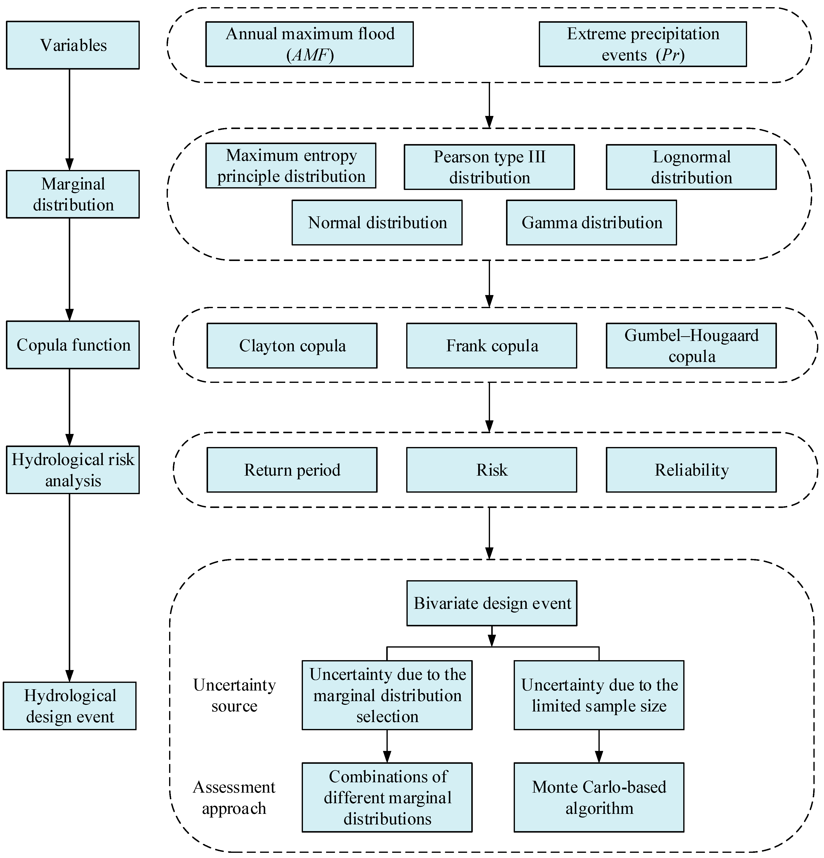
Figure 3.
Experimental design for assessing the uncertainty of marginal distribution in bivariate design event estimation.
Figure 3.
Experimental design for assessing the uncertainty of marginal distribution in bivariate design event estimation.

Figure 4.
Frequency distributions of the AMF and Pr series in the upper catchments of Linjiacun and Huaxian stations. (A,C,E,G) denote the cumulative probabilities of the AMF and Pr series, while (B,D,F,H) denote the probability density of the AMF and Pr series.
Figure 4.
Frequency distributions of the AMF and Pr series in the upper catchments of Linjiacun and Huaxian stations. (A,C,E,G) denote the cumulative probabilities of the AMF and Pr series, while (B,D,F,H) denote the probability density of the AMF and Pr series.


Figure 5.
Bivariate return periods for (AMF, Pr) pairs in the upper catchments of Linjiacun and Huaxian stations. (A,C) denote the joint return period for the “OR” case, while (B,D) denote the joint return period for the “AND” case.
Figure 5.
Bivariate return periods for (AMF, Pr) pairs in the upper catchments of Linjiacun and Huaxian stations. (A,C) denote the joint return period for the “OR” case, while (B,D) denote the joint return period for the “AND” case.

Figure 6.
Bivariate risk and reliability under different designed (AMF, Pr) pairs when the hydraulic project life is given as 10 years. (A,C) denote the bivariate risk under different (AMF, Pr) pairs in the upper catchments of Linjiacun and Huaxian stations, respectively, while (B,D) denote the bivariate reliability under different (AMF, Pr) pairs for the two regions, respectively.
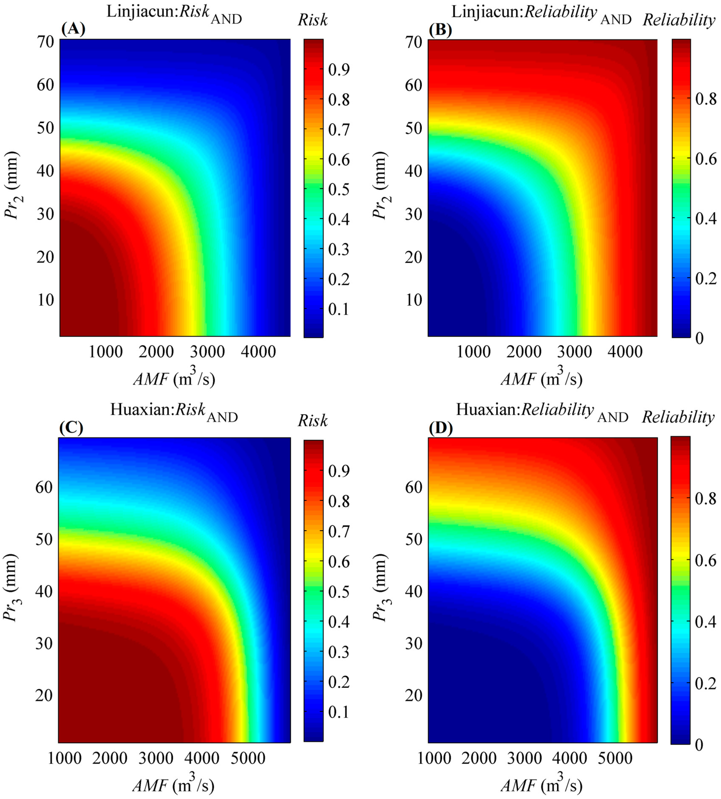
Figure 7.
Most-likely design events under different combinations of marginal distributions. (A,C) denote the most likely design events under different combinations of marginal distributions when TOR = 30 years in the upper catchments of Linjiacun and Huaxian stations, respectively, while (B,D) denote the most likely design events when TAND = 30 years in the two regions, respectively.

Figure 8.
Part of CDF curves for AMF (A) and Pr (B) series in the upper catchment of Linjiacun station.
Figure 8.
Part of CDF curves for AMF (A) and Pr (B) series in the upper catchment of Linjiacun station.
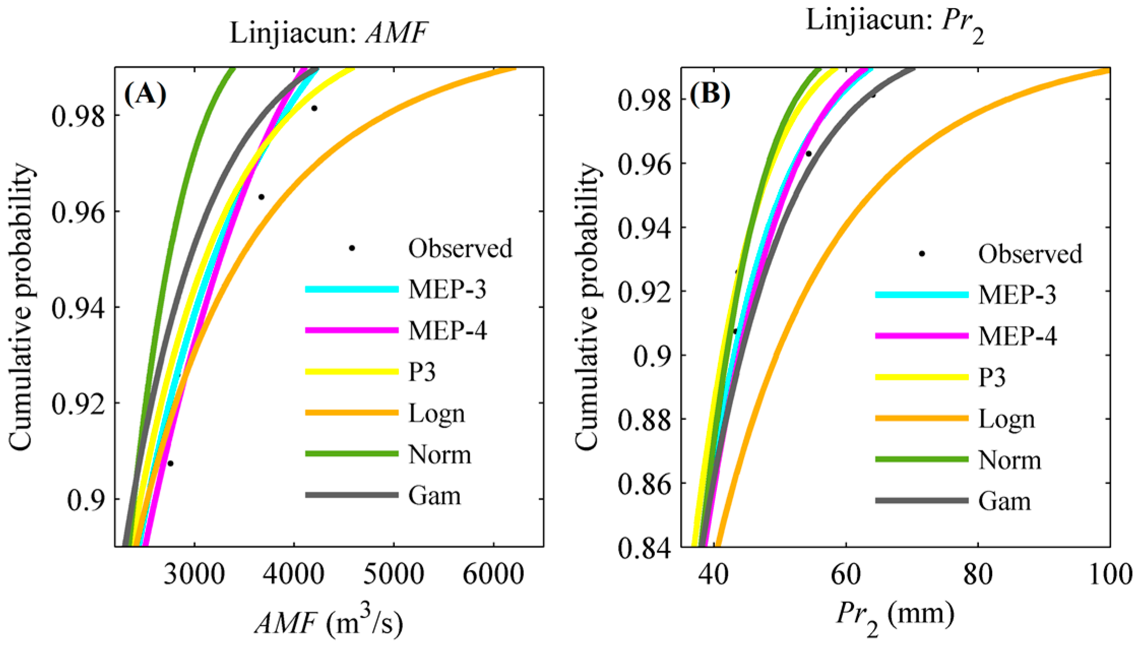
Figure 9.
The most-likely design events with the “OR” (A,C) and “AND” (B,D) joint period of 30 years. Black lines denote the “OR” and “AND” joint periods estimated with the original data series. The shaded area denotes the confidence regions of the most-likely design events with TOR = TAND = 30 years at 95% and 99% confidence interval.

Table 1.
Correlation coefficients between AMF and Pr. Bold numbers denote the extreme precipitation events most correlated with AMF.
Table 1.
Correlation coefficients between AMF and Pr. Bold numbers denote the extreme precipitation events most correlated with AMF.
| Station | Correlation Coefficient | ||||
|---|---|---|---|---|---|
| (AMF, Pr1) | (AMF, Pr2) | (AMF, Pr3) | (AMF, Pr4) | (AMF, Pr5) | |
| Linjiacun | 0.1420 | 0.4192 ** | 0.3654 ** | 0.3582 ** | 0.3320 ** |
| Huaxian | 0.1586 | 0.2369 * | 0.3756 ** | 0.3175 ** | 0.3320 ** |
Note: * and ** indicate that correlation coefficients are significant at the 95% and 99% confidence level, respectively.
Table 2.
Parameters of the fitted distribution for the AMF and Pr series in the catchments of Linjiacun and Huaxian stations.
Table 2.
Parameters of the fitted distribution for the AMF and Pr series in the catchments of Linjiacun and Huaxian stations.
| Distribution | Parameter | Linjiacun | Huaxian | |||
|---|---|---|---|---|---|---|
| AMF | Pr2 | AMF | Pr3 | |||
| MEP-3 | f (x|λ1, λ2, λ3) | λ1 | 4.04 × 10⁻⁴ | −0.15 | 3.50 × 10⁻³ | −0.15 |
| λ2 | 2.64 × 10⁻⁷ | 4.65 × 10⁻³ | −1.14 × 10⁻⁶ | 4.01 × 10⁻³ | ||
| λ3 | −4.02 × 10⁻¹¹ | −2.93 × 10⁻⁵ | 1.19 × 10⁻¹⁰ | −2.25 × 10⁻⁸ | ||
| MEP-4 | f (x|λ1, λ2, λ3, λ4) | λ1 | 7.63 × 10⁻⁴ | −0.23 | −3.20 × 10⁻⁴ | 0.07 |
| λ2 | 1.57 × 10⁻⁶ | 9.65 × 10⁻³ | 1.03 × 10⁻⁶ | −6.73 × 10⁻³ | ||
| λ3 | −5.40 × 10⁻¹⁰ | −1.48 × 10⁻⁴ | −3.73 × 10⁻¹⁰ | −1.87 × 10⁻⁴ | ||
| λ4 | 6.01 × 10⁻¹⁴ | 9.13 × 10⁻⁷ | 3.83 × 10⁻¹⁴ | −1.41 × 10⁻⁶ | ||
| P3 | f (x|a, b, α) | a | 1.23 | 13.19 | 0.99 | 21.65 |
| b | 88.08 | −22.69 | 866 | −26.25 | ||
| α | 880.82 | 3.56 | 1999.35 | 2.57 | ||
| Logn | f (x|μ, σ) | μ | 6.73 | 3.01 | 7.82 | 3.29 |
| σ | 0.86 | 0.69 | 0.56 | 0.44 | ||
| Norm | f (x|μ, σ) | μ | 1170.32 | 24.52 | 2853.66 | 29.54 |
| σ | 954.42 | 13.55 | 1413.64 | 12.7 | ||
| Gam | f (x|μ, σ) | μ | 1.65 | 2.82 | 3.71 | 5.53 |
| σ | 707.28 | 8.68 | 770.06 | 5.34 | ||
Note: PDF of P3: ; PDF of Logn: ; PDF of Norm: ; PDF of Gam: , where is a complete gamma function.
Table 3.
The goodness-of-fit and RMSE values of the candidate distributions for the AMF and Pr series in the study regions.
Table 3.
The goodness-of-fit and RMSE values of the candidate distributions for the AMF and Pr series in the study regions.
| Station | Series | Functions | K-S Test | RMSE | Series | Functions | K-S Test | RMSE | ||
|---|---|---|---|---|---|---|---|---|---|---|
| S | p | S | p | |||||||
| Linjiacun | AMF | MEP-3 | 0.09 | 0.72 | 0.0303 | Pr2 | MEP-3 | 0.08 | 0.89 | 0.0293 |
| MEP-4 | 0.07 | 0.85 | 0.0296 | MEP-4 | 0.07 | 0.95 | 0.0248 | |||
| P3 | 0.08 | 0.85 | 0.0309 | P3 | 0.09 | 0.80 | 0.0373 | |||
| Logn | 0.09 | 0.80 | 0.0366 | Logn | 0.10 | 0.58 | 0.0450 | |||
| Norm | 0.15 | 0.19 | 0.0823 | Norm | 0.12 | 0.43 | 0.0473 | |||
| Gam | 0.11 | 0.53 | 0.0405 | Gam | 0.08 | 0.87 | 0.0275 | |||
| Huaxian | AMF | MEP-3 | 0.06 | 0.98 | 0.0195 | Pr3 | MEP-3 | 0.09 | 0.73 | 0.0306 |
| MEP-4 | 0.06 | 0.97 | 0.0202 | MEP-4 | 0.08 | 0.78 | 0.0267 | |||
| P3 | 0.14 | 0.25 | 0.0686 | P3 | 0.10 | 0.65 | 0.0299 | |||
| Logn | 0.10 | 0.59 | 0.0553 | Logn | 0.10 | 0.62 | 0.0390 | |||
| Norm | 0.12 | 0.37 | 0.0534 | Norm | 0.09 | 0.76 | 0.0382 | |||
| Gam | 0.09 | 0.74 | 0.0513 | Gam | 0.10 | 0.63 | 0.0300 | |||
Table 4.
Parameters and goodness-of-fit test values for the candidate copulas.
| Station | Copula | Parameter | Cramér–von Mises Test | AICc | |
|---|---|---|---|---|---|
| Sn | p-Value | ||||
| Linjiacun | Clayton | 0.31 | 0.03 | 0.23 | −10.83 |
| Frank | 4.09 | 0.04 | 0.10 | −19.54 | |
| Gumbel | 1.59 | 0.03 | 0.15 | −22.38 | |
| Huaxian | Clayton | 0.42 | 0.03 | 0.45 | −11.67 |
| Frank | 3.72 | 0.02 | 0.59 | −17.03 | |
| Gumbel | 1.50 | 0.03 | 0.36 | −16.22 | |
Table 5.
Most-likely design events under different combinations of marginal distributions.
| Distribution | Most-Likely Design Event (AMF, Pr) | ||||
|---|---|---|---|---|---|
| TOR = 30 | TAND = 30 | ||||
| AMF | Pr | Linjiacun | Huaxian | Linjiacun | Huaxian |
| MEP-3 | MEP-3 | (3921.34, 56.26) | (5626.03, 63.42) | (2877.37, 46.53) | (4976.51, 42.52) |
| MEP-4 | (3920.99, 56.72) | (5369.10, 73.46) | (2864.31, 48.00) | (5017.84, 41.64) | |
| P3 | (3937.32, 57.06) | (5653.22, 55.68) | (2921.17, 46.92) | (4924.88, 41.07) | |
| Logn | (3930.55, 78.62) | (5678.83, 64.63) | (3065.06, 56.57) | (5028.83, 39.38) | |
| Norm | (3961.55, 51.29) | (5642.49, 54.98) | (2760.59, 44.54) | (4882.04, 42.83) | |
| Gam | (3925.95, 60.35) | (5660.16, 59.29) | (2960.32, 48.86) | (4966.30, 40.87) | |
| MEP-4 | MEP-3 | (3833.86, 57.87) | (5492.61, 65.46) | (3105.70, 45.48) | (4969.43, 42.53) |
| MEP-4 | (3825.82, 56.95) | (5290.03, 73.46) | (3052.79, 46.76) | (4991.76, 41.49) | |
| P3 | (3849.07, 52.66) | (5521.30, 56.98) | (3034.24, 42.96) | (4928.09, 40.94) | |
| Logn | (3834.21, 79.18) | (5539.27, 67.13) | (3204.83, 54.23) | (5010.76, 39.49) | |
| Norm | (3849.58, 51.53) | (5513.93, 56.04) | (2980.19, 43.39) | (4894.56, 42.64) | |
| Gam | (3830.33, 60.66) | (5526.09, 60.98) | (3126.29, 47.38) | (4960.69, 40.82) | |
| P3 | MEP-3 | (3828.15, 57.44) | (8613.13, 67.16) | (2772.63, 47.11) | (4897.99, 49.50) |
| MEP-4 | (3842.96, 57.74) | (7635.10, 73.46) | (2750.37, 48.44) | (5372.34, 46.50) | |
| P3 | (3860.18, 58.30) | (8866.89, 57.89) | (2802.71, 47.44) | (4591.65, 46.52) | |
| Logn | (3867.76, 81.16) | (8984.54, 68.75) | (2936.73, 57.73) | (5204.69, 46.98) | |
| Norm | (3868.93, 52.20) | (8820.36, 56.80) | (2654.70, 44.82) | (4400.06, 47.56) | |
| Gam | (3853.61, 61.71) | (8897.28, 62.14) | (2839.67, 49.46) | (4809.40, 47.38) | |
| Logn | MEP-3 | (4609.04, 57.71) | (7749.23, 67.64) | (2843.58, 48.19) | (4499.62, 49.81) |
| MEP-4 | (4636.79, 57.96) | (6941.66, 73.46) | (2807.61, 49.49) | (4890.92, 46.87) | |
| P3 | (4665.66, 58.58) | (7989.66, 58.14) | (2898.54, 48.52) | (4289.21, 46.69) | |
| Logn | (4670.78, 81.59) | (8094.99, 69.23) | (3141.70, 60.07) | (4729.38, 47.43) | |
| Norm | (4681.88, 52.44) | (7948.81, 57.00) | (2618.77, 45.66) | (4155.63, 47.64) | |
| Gam | (4653.58, 61.99) | (8017.00, 62.46) | (2969.72, 50.66) | (4437.30, 47.64) | |
| Norm | MEP-3 | (3108.07, 57.79) | (5793.91, 66.33) | (2524.13, 44.13) | (4699.00, 44.79) |
| MEP-4 | (3119.85, 58.02) | (5446.16, 73.46) | (2497.94, 45.68) | (4782.48, 43.07) | |
| P3 | (3130.51, 58.61) | (5861.15, 57.45) | (2534.21, 44.25) | (4606.08, 43.07) | |
| Logn | (3152.78, 82.35) | (5898.04, 67.97) | (2603.77, 47.62) | (4797.38, 41.64) | |
| Norm | (3124.46, 52.27) | (5846.46, 56.43) | (2481.91, 43.14) | (4535.18, 44.65) | |
| Gam | (3132.06, 62.18) | (5870.99, 61.58) | (2542.46, 45.41) | (4676.33, 43.10) | |
| Gam | MEP-3 | (3586.49, 57.56) | (6654.48, 66.89) | (2633.78, 46.68) | (4677.02, 47.24) |
| MEP-4 | (3601.58, 57.84) | (6096.07, 73.46) | (2604.74, 48.09) | (4883.48, 44.83) | |
| P3 | (3617.00, 58.41) | (6785.93, 57.75) | (2660.38, 46.99) | (4515.48, 44.90) | |
| Logn | (3632.96, 81.57) | (6850.96, 68.51) | (2769.53, 56.15) | (4846.30, 44.36) | |
| Norm | (3620.10, 52.24) | (6760.41, 56.68) | (2540.92, 44.61) | (4401.43, 46.19) | |
| Gam | (3613.57, 61.86) | (6803.04, 61.96) | (2687.53, 48.87) | (4631.91, 45.35) | |
© 2017 by the authors. Licensee MDPI, Basel, Switzerland. This article is an open access article distributed under the terms and conditions of the Creative Commons Attribution (CC BY) license (http://creativecommons.org/licenses/by/4.0/).
Share and Cite
MDPI and ACS Style
Guo, A.; Chang, J.; Wang, Y.; Huang, Q.; Guo, Z. Maximum Entropy-Copula Method for Hydrological Risk Analysis under Uncertainty: A Case Study on the Loess Plateau, China. Entropy 2017, 19, 609. https://doi.org/10.3390/e19110609
AMA Style
Guo A, Chang J, Wang Y, Huang Q, Guo Z. Maximum Entropy-Copula Method for Hydrological Risk Analysis under Uncertainty: A Case Study on the Loess Plateau, China. Entropy. 2017; 19(11):609. https://doi.org/10.3390/e19110609
Chicago/Turabian StyleGuo, Aijun, Jianxia Chang, Yimin Wang, Qiang Huang, and Zhihui Guo. 2017. "Maximum Entropy-Copula Method for Hydrological Risk Analysis under Uncertainty: A Case Study on the Loess Plateau, China" Entropy 19, no. 11: 609. https://doi.org/10.3390/e19110609
Note that from the first issue of 2016, this journal uses article numbers instead of page numbers. See further details here.