Modal Strain Energy-Based Debonding Assessment of Sandwich Panels Using a Linear Approximation with Maximum Entropy


Department of Mechanical Engineering, Universidad de Chile, Beauchef 851, Santiago 7591538, Chile
*
Author to whom correspondence should be addressed.
Entropy 2017, 19(11), 619; https://doi.org/10.3390/e19110619
Submission received: 21 September 2017
/
Revised: 5 November 2017
/
Accepted: 14 November 2017
/
Published: 17 November 2017
(This article belongs to the Special Issue Entropy for Characterization of Uncertainty in Risk and Reliability)
Abstract
:Sandwich structures are very attractive due to their high strength at a minimum weight, and, therefore, there has been a rapid increase in their applications. Nevertheless, these structures may present imperfect bonding or debonding between the skins and core as a result of manufacturing defects or impact loads, degrading their mechanical properties. To improve both the safety and functionality of these systems, structural damage assessment methodologies can be implemented. This article presents a damage assessment algorithm to localize and quantify debonds in sandwich panels. The proposed algorithm uses damage indices derived from the modal strain energy method and a linear approximation with a maximum entropy algorithm. Full-field vibration measurements of the panels were acquired using a high-speed 3D digital image correlation (DIC) system. Since the number of damage indices per panel is too large to be used directly in a regression algorithm, reprocessing of the data using principal component analysis (PCA) and kernel PCA has been performed. The results demonstrate that the proposed methodology accurately identifies debonding in composite panels.
1. Introduction
Sandwich structures typically consist of thin face sheets or skins and a lightweight thicker core, which is sandwiched between the skins to obtain a structure of superior bending stiffness. The concept of sandwich is a common principle in nature. For example, the branches of trees or the bones in skeletons are examples of sandwich structures with foam-like core materials. The high stiffness and low weight of sandwich structures make them attractive in applications where weight reduction is critical. Consequently, the applications of sandwich structures have grown rapidly in recent years, for example in satellites, spacecraft, aircraft, ships, automobiles, rail cars, wind energy systems, and bridge construction [1].
Notwithstanding, these structures may present imperfect bonding or debonding between the skins and core as a result of manufacturing defects or impact loads. Debonding in a sandwich structure may severely degrade its mechanical properties, which can produce a catastrophic failure of the structure. Therefore, although in aircraft design it is fundamental to make a structure as light as possible without sacrificing strength, sandwich structures remain limited to secondary (non-critical) components [2].
Structural damage assessment methodologies can be implemented to increase both the safety and functionality of these systems. The objective of damage assessment is to detect and characterize damage as early as possible, and to estimate the time required for the structure to fail. This entails life safety and economic benefits by increasing the safety and reliability of the structure and reducing maintenance costs.
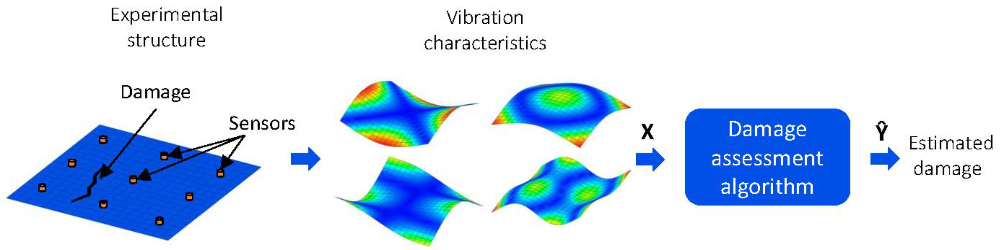
There has been an increase in the number of vibration-based damage assessment methods in recent years [3]. The fundamental principle of these assessment methods is that vibration characteristics, such as natural frequencies, mode shapes, and modal damping, depend on the physical properties of the structure. Therefore, any change to the physical properties due to damage will produce measurable changes in the vibration characteristics. The principle of a vibration-based damage assessment algorithm is illustrated in Figure 1; the inputs are the vibration characteristics of the structure, and the output is the estimated damage.
Different studies have confirmed that vibration characteristics are sensitive to debonding in sandwich structures. The first numerical investigation was performed by Jiang et al. [4] who modelled debonded honeycomb structures with commercial finite element software. Their results showed that natural frequencies are good indicators of the presence of debonding. The finite element method was also used by Burlayenko et al. [5,6] to study the influence of skin/core debonding on the vibrations of honeycomb panels, concluding that the size of the debonded zone reduces the natural frequencies and creates a discontinuity in the mode shapes. Similar conclusions have been found in the experimental and theoretical/numerical investigations of Kim and Hwang [7] and Lou et al. [8], where it was concluded that natural frequencies decrease due to loss of stiffness caused by local damage and that vibration modes show local deformation in the damaged region. On the other hand, the experimental study performed by Shahdin et al. [9] showed that the damping ratio is a more sensitive parameter for damage detection than the natural frequencies, although it is much harder to estimate.
Vibration-based damage assessment methods are categorized as model-based or non-model-based. Non-model-based methods compare the undamaged and damaged measurements to detect damage, whereas model-based methods combine an analytical model with experimental measurements to locate and quantify damage. In addition, model-based methods are useful for predicting the structure’s response to new loading conditions and/or new system configurations (damage states), which allows for damage prognosis [10]. Model-based damage assessment requires the solution of a nonlinear inverse problem, which can be accomplished by model updating algorithms based on global optimization [11]. However, these algorithms can become very slow, hindering applications in real time.
Supervised learning algorithms are an alternative to model updating. They have the objective of estimating the structure’s damage state based on current and past measurements. Supervised learning is classified into two classes: parametric supervised learning, that assumes a statistical model for the data samples, and non-parametric supervised learning, that does not assume a structure for the data. The most frequently used nonparametric algorithms are artificial neural networks (ANNs). Islam and Craig [12] used the natural frequencies of a composite beam to train a neural network that determines the location and size of the delamination. The natural frequencies were identified using modal analysis and piezoceramic patches acting as both sensors and actuators. Okafor et al. [13] presumed that the delamination of a composite beam was located at its middle and predicted the delamination size using a neural network trained with the natural frequencies. The prediction was accurate for dimensionless delamination sizes between 0.22 and 0.82. Similarly, Valoor and Chandrashekhara [14] identified delamination locations and sizes in a thick composite beam using neural network and natural frequencies. They found that the larger errors are obtained with delaminations near the beam ends, and that in symmetrical structures the network can only predict the probable location in each symmetrical section. Therefore, to localize delamination in symmetrical structures, more information, such as mode shape, is required. Ishak et al. [15] trained a neural network with displacements of a laminated composite beam measured by a scanning laser vibrometer to predict location, depth and length of delamination. Chakraborty [16] predicted the size and location of delamination in composite panels using natural frequencies and neural networks. The method was verified with simulated data showing that the network performs satisfactorily. Nevertheless, according to the authors it is necessary to test the actual efficacy of the algorithm with experimental data. Su et al. [17] evaluated the performance of neural networks and genetic algorithms (GAs) in assessing delamination in composite beams using natural frequencies. The authors concluded that both algorithms were able to correctly identify the delamination, but neural networks are more stable. Zhang et al. [18,19] compared three inverse algorithms to predict the location and size of delamination in a composite beam, namely, a graphical technique, neural networks, and surrogate-assisted optimization. The three algorithms could predict the delamination parameters, but neural networks were found to be less reliable in the presence of experimental noise.
Once a neural network is already trained, it can quickly process new data, making it useful for real-time damage assessment. Nevertheless, the slow learning speed and the large number of parameters that need to be selected during the training phase have been an obstacle to their application [20]. A new supervised learning algorithm, denoted LME (linear approximation with maximum entropy), which uses a linear approximation based on the maximum-entropy principle, was developed by Meruane and Ortiz-Bernardin [21]. The advantages of LME over current methods are multiple: it requires the selection of only one parameter; it has a unique solution; and can process the data with a similar speed to ANNs. Furthermore, the LME performs linear interpolation using the training data to estimate the damage, which does not require classical training. The principal advantage is that new data can be easily incorporated into the training database with no need to re-train the algorithm as in the case of ANNs. The LME algorithm was first developed for damage assessment [21,22], and Sanchez et al. [23] and Meruane et al. [24] employed it in impact identification.
There are many response parameters that have been used in damage assessment, including natural frequencies [25], the modal assurance criterion (MAC) [11], the spatial correlation of mode shapes (COMAC) [26], mode shape curvatures [27], modal flexibility and its derivatives [28,29], and modal strain energy (MSE) [30] among others. Most of them have been developed for one-dimensional structures, such as beams, frames and truss structures. Comparatively, there are only few studies on damage assessment of two-dimensional (plate-like) structures. Cornwell et al. [31] were the first to use the strain energy in a damage localization method for plate-like structures. The damage index was computed using the strain energy of a plate in the undamaged and damaged states. The method was validated using numerical simulations with experimental data of an aluminum plate with saw cuts. Lin et al. [32] investigated the identification of damage in plate-like structures using a strain mode technique derived from a Rayleigh–Ritz approach. The authors proposed two damage indices: the bending moment index, and the residual strain mode shape index. Their results show that the bending moment is more sensitive than the strain mode shape, but the detection depends on the damage location, whereas the residual strain mode shape detects damage accurately independent of the location. Wu and Law [33] developed a damage localization method for plate structures based on changes in the uniform load-surface (ULS) curvature. ULS is defined as the deflection vector of a structure under a uniform load. The method was validated with numerical data of different plates, and damage was introduced as a localized stiffness reduction. In a later work, Wu and Law [34] proposed a model-based damage assessment algorithm that also used changes in the ULS curvature. The inverse problem was modelled as a linear equation system based on a first-order Taylor series approximation and was solved iteratively. Yoon et al. [35] presented a baseline-free damage localization algorithm for plate-like structures. The algorithm used vibration mode curvatures and a 2D gapped smoothing (GS) method to locate changes in structural stiffness. The condition for damage location without baseline data was that the structure was homogeneous with respect to stiffness in the undamaged case. Qiao et al. [36] studied the experimental identification of delamination in a composite laminate plate using three different methodologies: GS, generalized fractal dimension, and modal strain energy (MSE). Experimental data were measured using two approaches: the scanning laser vibrometer (SLV) and the polyvinylidene fluoride (PVDF) sensor. The results show that an SLV provides better results than a PVDF sensor because of its refined scanning mesh. However, although all the three methods can detect the actual location of damage, they also show extra peaks at other locations (false damage). The authors concluded that the GS method identifies the delamination of composite plates better than other algorithms. Moreno-García et al. [37] investigated the use of higher-order mode shape derivatives to locate damage in plate-like structures. The authors concluded that a damage indicator based on the fourth-order spatial derivative allows better damage localization. In addition, as the number of measured degrees of freedom (DOFs) increases, the success in damage localization also increases. Chang and Chen [38] developed an algorithm that uses the spatial wavelet analysis for damage detection in a two-dimensional structure. They use the wavelet coefficients of the mode shapes, computed by a 1D continuous wavelet transform (CWT), to detect local perturbations caused by damage. The proposed algorithm was validated with simulated data of a rectangular plate, showing that the wavelet analysis of the mode shapes is sensitive to the damage size. The 1D CWT with different wavelets was applied by Douka et al. [39] to detect cracks in plates. The method was validated with numerically simulated data of a plate with a crack. The 2D CWT has been implemented in different investigations to identify damage in two-dimensional experimental and numerical structures [40,41,42,43]. Katunin [44] introduced the discrete wavelet transform (DWT) together with B-splines wavelets for damage identification in composite plates. The author proved that DWT with B-splines provides comparable results at lower processing times than CWT approaches. Further studies were carried out on composite plates with artificial damage to determine the optimal selection of wavelet parameters [45] and in the implementation of fractional discrete wavelet transform (FrDWT) to identify damage in honeycomb-core sandwich composite structures [46]. Seguel [47] investigated the application of full-field vibration measurements in the debonding assessment of an aluminum honeycomb sandwich panel. Experimental data was acquired by a high-speed 3D DIC system, and four methodologies to compute damage indices were evaluated: mode shape curvatures, uniform load surface, modal strain energy, and gapped smoothing. The results demonstrated that a high-speed 3D system can be used to successfully identify debonding in composite panels. Among the four methodologies evaluated by Seguel, the best results were obtained with the MSE method.
The damage assessment algorithms for two-dimensional structures presented above provide a qualitative estimate of the damage given by maps of the distribution of damage indices over the structure. The present article investigates the application of the modal strain energy method in conjunction with the LME algorithm to deliver a quantitative estimation of the debonding of honeycomb sandwich panels. This is achieved by training the LME algorithm to estimate the location and size of the damage using as input the map of damage indices. Full-field vibration measurements of the panels are acquired by a high-speed 3D digital image correlation (DIC) system. The principal advantages of DIC over conventional vibration measurements are: (1) the high spatial resolution; (2) there is no contact and no mass loading; and (3) the low sensitivity to rigid body motion [48]. Since the number of damage indices per panel was too large to be used directly in a regression algorithm, reprocessing of the data using principal component analysis (PCA) and kernel PCA was performed.
Supervised learning algorithms require large data training sets. Nevertheless, it is very difficult and time-consuming to produce enough data sets from experiments. Alternatively, the data sets can be generated using a numerical model of the structure. It has been demonstrated by diverse studies that it is possible to produce correct damage predictions in an experimental structure using supervised learning algorithms trained with data obtained from a numerical model [20,21,22,49]. Here, a finite element model of the panel was used to generate the data to train the damage assessment algorithm.
The rest of this work is structured as follows: Section 2 presents the proposed damage assessment algorithm; Section 3 describes the methodology followed during the implementation of the algorithm; Section 4 describes the application case under investigation; Section 5 presents the damage assessment results; and finally, the conclusions and forthcoming work are presented in Section 6.
2. Damage Assessment Algorithm
2.1. Damage Parameterization
Damage is modeled by circular-shaped debonded regions represented by the vector , where are the x and y coordinates of the center of the debonded region and is the radius of the debonded region, as illustrated in Figure 2.
2.2. Damage Indices
The modal strain energy has shown to be a sensitive indicator of damage and it has been frequently used to locate damage in one-dimensional structures such as beams, frames and truss structures [30]. Cornwell et al. [31] introduced the strain energy damage detection method for plate-like structures. The damage indices are computed using the modal strain energy of a plate in the undamaged and damaged states. In the case of a plate-like structure, for a particular mode shape, , the strain energy associated with that mode shape is
where a and b are the plate dimensions, and is the bending stiffness of the plate. By dividing the plate in sub-regions, it is possible to locate damage by comparing the normalized strain energy of each sub-region in the undamaged and damaged conditions. The energy associated with sub-region jk for the r-th mode shape is given by
Therefore
where Nx and Ny are the number of divisions of the x and y directions, respectively. The fractional energy at location jk is
The same procedure can be used to compute the fractional energy at location jk for the r-th mode of the damaged structure, . To account for all measured modes, the damage index for sub-region jk is defined as
where m is the number of measured modes. Assuming that the collection of damage indices represents a population of normally distributed random variables, a normalized damage index is obtained using
where and represent the mean and standard deviation of the damage indices, respectively.
The damage indices of the i-th panel are arranged in the vector as follows:
where and is the damage index at the position jk of the i-th panel.
The proposed methodology uses three databases: one for training, one to set up the parameters of the damage assessment algorithm, and one to evaluate the algorithm. The damage indices of the panels are arranged as the columns of the matrices , and , representing the panels in the training, setting-up and testing databases, respectively.
2.3. Principal Component Analysis
The objective of PCA is to reduce the dimensionality of a data set while retaining the variation present in the data set as much as possible. This is achieved by transforming it to a new set of uncorrelated variables known as the principal components (PCs).
PCA is defined as an orthogonal linear transformation that transforms the data to a new coordinate system such that the greatest variance by any projection lies on the first PC, the second greatest variance on the second PC, and so on.
Let be a data matrix with the damage indices of the training database. In general, it is recommended to normalize the data before performing PCA. This is because some of the variables might have a large variance while others might have a small variance, and the variables with a large variance will dominate the first PCs. Nevertheless, in this case the input data has already been normalized, as presented in Equation (6).
The goal of PCA is to find a matrix , such that a linear mapping from the original dimension p to a lower dimension n is provided. A new matrix , called the score matrix, is obtained from
P can be calculated by extracting the main n eigenvectors of the covariance matrix of , C, which is given by
The j-th column of corresponds to the PCs associated with the j-th panel in the training database. The PCs of the panels in the setting-up and testing databases are computed using the same transformation matrix P:
2.4. Kernel PCA
Standard PCA only allows linear dimensionality reduction. However, if the data cannot be represented well in a linear subspace, standard PCA will not be effective. Kernel PCA generalizes PCA to nonlinear dimensionality reduction [50,51].
Let us define a nonlinear transformation, from the original p-dimensional space to an m-dimensional space. corresponds to the i-th columns of the matrix . The covariance matrix of the projected features is
We have to find the eigenvalues and eigenvector V satisfying . The solutions for V lie in the span . Therefore, the following equivalent system can be formulated:
and there exist coefficients such that
Substituting Equations (14) and (12) into Equation (13) we have,
where denotes the column vector with entries , and the matrix kernel is defined as
The vector can be solved by
To extract the principal components, the test points are projected onto the matrix that contains the main n eigenvectors according to
If the projected data set does not have zero mean, the kernel matrix is substituted with the Gram matrix
where is the matrix with all elements equal to 1/p.
2.5. Linear Approximation with Maximum Entropy (LME)
The observation vector, , contains information related to the damage location and magnitude for the j-th scenario in the training database, as described in Section 2.1. The feature vector , which is obtained from the j-th column of in Equation (8) or (18), represents the set of PCs associated to the j-th observation vector . Assuming that a training database with a set of N panels is constructed, each panel is characterized by an observation vector and a feature vector. Therefore, the database is formed by N pairs of observation and feature vectors as: . The central calculation in damage assessment is that given a certain feature , the corresponding observation should be estimated. The nearest-neighbor regression estimate of is given by
where are the observation vectors associated with the k-closest neighbors to the test vector , and are weighting functions. The k-nearest-neighbor (k-NN) algorithm weights each neighbor equally, thus , for i = 1 to k. In contrast, a kernel nearest-neighbor algorithm bases weightings on the distance from the test vector to each vector in the database [52].
On the other hand, linear approximation takes the N feature vectors in the database and uses a linear combination of them to represent as
where are the feature vectors in the training database. Once the weighting functions are determined, is estimated from Equation (23) with k = N. Typically Equation (24) is undetermined and its solution can be tackled via an unconstrained optimization technique of the family of least-squares. However, these methods produce some negative weights, which lack physical meaning. An alternative that produces positive weights is obtained via the maximum-entropy (max-ent) variational principle. In that case, the optimization problem that builds the damage assessment algorithms reads as follows:
subject to the constraints
where has been introduced as a shifted measure for stability purposes. Although different prior distributions can be used, in damage assessment the best performance was obtained with a smooth Gaussian [21],
where ; is a parameter that controls the support of the Gaussian prior at and therefore its associated weight function; and is a characteristic n−dimensional Euclidean distance between neighbors that can be distinct for each . In view of the optimization problem posed in Equation (24) for supervised learning, maximizing the entropy requires a weight solution that commits the least to all of the database samples [53].
The solution of the max-ent optimization problem is handled by using the procedure of Lagrange multipliers, which yields [54]:
where , , and are the converged Lagrange multipliers.
In Equation (28), the Lagrange multiplier vector is the minimizer of the dual optimization problem posed in Equation (29) [54]:
which gives rise to the following system of nonlinear equations:
where stands for the gradient with respect to . Once the converged is found, the weight functions are computed from Equation (28), and the damage is estimated from Equation (23) with k = N.
3. Methodology
The damage assessment methodology consists of four main parts: (1) building of the databases; (2) selection of parameters; (3) evaluation of the algorithm; and (4) experimental validation.
3.1. Building of the Databases
Three databases are constructed: the training database, the setting-up database and the testing database. The damage is modelled with circular-shaped debonded regions. The location and size of the debonded regions are defined randomly with dimensions between 0.001 and 0.1 m. The training, setting-up and testing databases consist of 3600, 30 and 200 individuals, respectively.
The PCs (computed either with PCA or kernel PCA) for the three databases are stored in the matrices , , and , respectively. The number of principal components are defined after a sentivity analysis to maximize the performance of the damage assessment algorithm as described in the next section.
3.2. Selection of Parameters
The parameters that need to be selected are: the number of neighbors that contribute to the solution, k; the number of principal components, n; and the parameter σ of the Gaussian kernel in kernel PCA. These parameters are selected to optimize the performance of the damage assessment algorithm. To quantify the performance, the following error functions are defined:
where is the number of elements in the database; and are the length of the panel in the x and y directions; and are the mean errors in the estimation of the debonding location in the x and y coordinates (localization errors); and is the percentage error in the estimation of the damage magnitude (quantification error).
3.3. Evaluation of the Algorithm
The next step is to evaluate the performance of the algorithm using the testing database. The procedure to assess damage consists of the following steps:
- (1)
- Extraction of a feature vector from the testing database.
- (2)
- Selection of the parameter in Equation (27), so that k neighbors contribute to the solution.
- (3)
- Solving of the system of nonlinear equations presented in Equation (30).
- (4)
- Computation of the weight functions using Equation (28).
- (5)
- Localization and quantification of the damage using Equation (23).
- (6)
- Computation of the localization and quantification errors using Equations (31)–(33).
- (7)
- Repetition of Steps 1–6 for all the feature vectors in the testing database.
3.4. Experimental Validation
The last step is experimental validation. The damage indices for the damaged panel are computed using the information of the undamaged and damaged panels as described in Section 2.2. Then, the PCs are computed using either PCA or kernel PCA and Steps (2) to (5) of Section 3.3 are followed to estimate the experimental damage.
4. Application Case
4.1. Experimental Measurements
The experimental structure consists of a sandwich panel measuring 0.25 × 0.35 × 0.021 m made of an aluminum honeycomb core bonded to two aluminum skins. The skins are bonded to the honeycomb core using an epoxy adhesive. Debonding is introduced as a circular region of radius 0.035 m without adhesive. To ensure perfect bonding, the panel is cured using a vacuum bagging system.
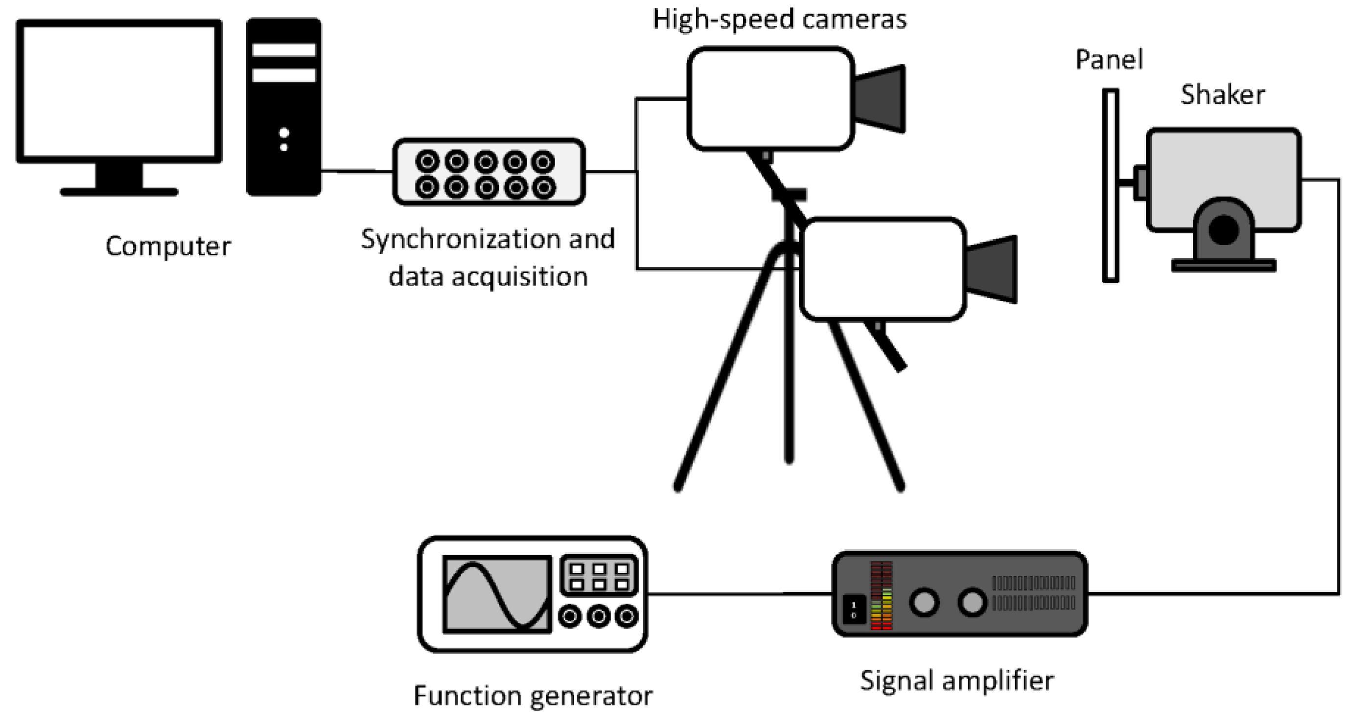
Figure 3 presents a scheme of the experimental setup; the panel is attached to an electrodynamic shaker, which is driven by a function generator and signal amplifier. The panel displacements are captured by two high-speed cameras, which are synchronized and connected to the digital image correlation software. The cameras, data acquisition, and digital image correlation software correspond to the Q450 high-speed DIC system from Dantec Dynamics.
To identify the experimental vibration mode shapes, the steps below are followed:
- First, the panel is excited in different points by an impact hammer and the response is captured by a miniature accelerometer. The experimental data are processed to obtain the frequency response functions (FRFs) from which the natural frequencies are identified by peak-picking.
- A speckle pattern is added to the panel by means of an adhesive sheet. This pattern provided by Dantec Dynamics has been optimized for DIC measurements. The cameras are calibrated and the image correlation parameters are selected to minimize the experimental error, following the recommendations given by Siebert et al. [55].
- In the case of high-speed DIC measurements, single-frequency excitation has shown to be the best method to identify experimental mode shapes [48,56]. Therefore, to identify mode shapes the shaker excites the panel with a sinusoidal vibration tuned at a natural frequency, causing the panel to vibrate in resonance. Images are captured at a rate of 5 kHz with a resolution of 1024 × 1024 pixels. Figure 4 show the vibration measurements with the high-speed DIC system and a vibration mode shape at 444 Hz.
- The experimental displacements are exported in hdf5 files, which are imported into Matlab. The Fourier transform of the displacements is computed and then the amplitude at the resonance frequency is recorded at each point. With this information, the operational mode shape at the resonant frequency is reconstructed.
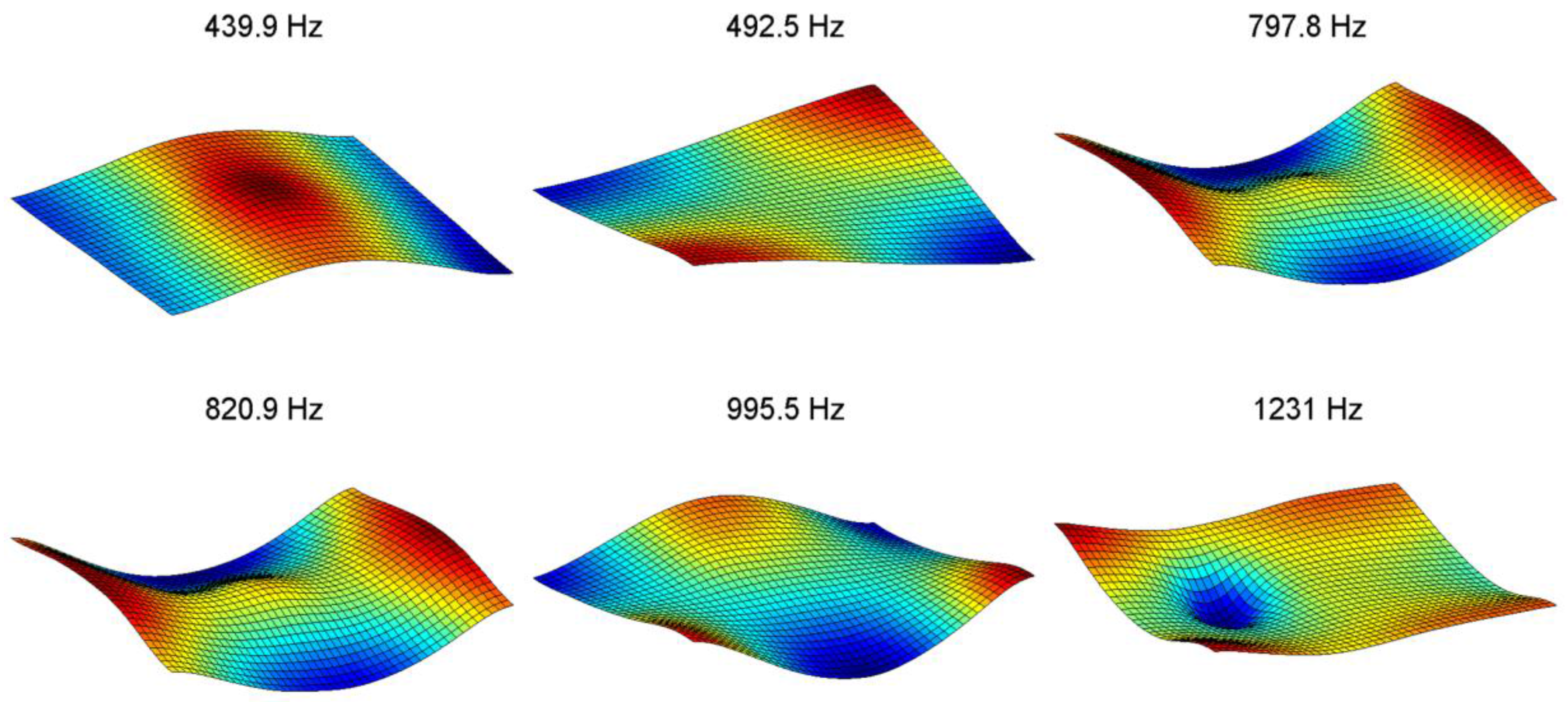
- Finally, the smoothing technique proposed by Garcia [21] is applied to reduce the experimental noise and to complete missing information in the mode shapes. Figure 5 and Figure 6 present the first six experimental model shapes for the undamaged and damaged panels. In both cases it is possible to see the effect of the shaker attachment in the middle of the panel. As expected, most of the natural frequencies of the damaged case are lower than the undamaged case. Regarding the mode shapes, the largest differences are found in the modes with higher frequencies.
4.2. Numerical Model
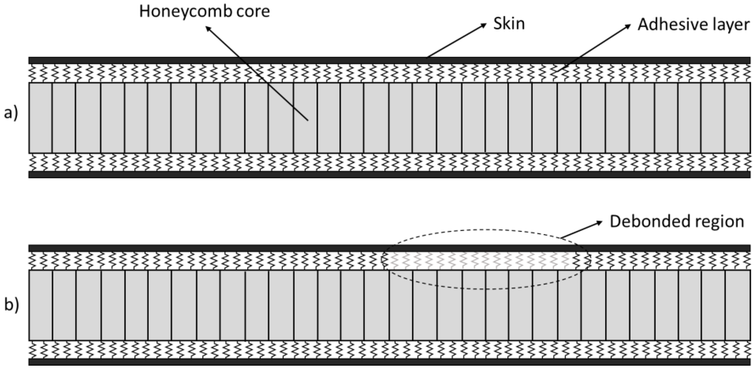
The training, setting-up and testing databases were built using a numerical model of the honeycomb panel, which was validated in [22]. The honeycomb panel is modelled with finite elements using a simplified three-layer shell model. The adhesive layer between the skin and core was modelled using linear springs, with reduced rigidity in debonded sectors, as shown in Figure 7.
The numerical model was built in Matlab® using the Structural Dynamics Toolbox (SDT) (Version 6.3) [57]; the skins and honeycomb panel were modelled with standard isotropic 4-node shell elements. The final model has 10,742 shell and 7242 spring elements.
The mechanical properties of the sandwich construction depend upon the adhesives, temperature and pressure used during curing. In addition, the anisotropic nature of the honeycomb core makes testing the sandwich specimens mandatory to determine their properties with accuracy. Here, the mechanical properties of the adhesive layer and the honeycomb core are determined by updating the finite element model with the experimental mode shapes and natural frequencies for both undamaged and damaged cases.
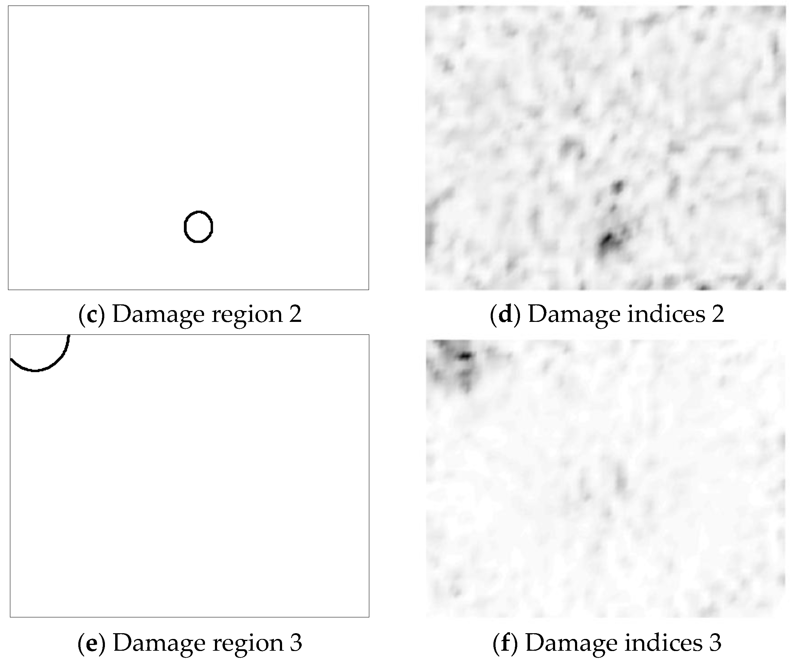
For each panel in the database, the first six mode shapes are identified and Equation (6) is used to obtain the distribution of damage indices through the panels. To simulate experimental measurements, the numerical modes are contaminated with random noise. The level of experimental noise expected in mode shapes identified by high-speed DIC measurements depends on the correlation error, the reconstruction error, and the numerical errors associated with the experimental modal analysis. From the results presented in [55,56], an estimation of 5% random noise seems reasonable. Figure 8 illustrates the damage indices obtained for three different scenarios. The pictures on the left show the damaged regions, whereas the pictures on the right show the distribution of damage indices through the panel.
5. Results
5.1. PCA + LME
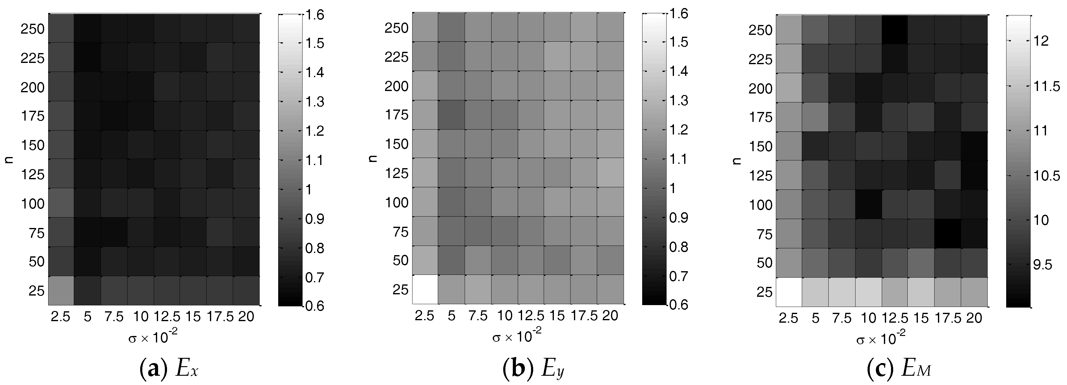
When applying PCA + LME there are two parameters that need to be defined: the number of PCs, n, and the number of neighbors contributing to the solution in the LME algorithm, k. To select those parameters, the damage assessment algorithm was evaluated using the setting-up database with different combinations of n and k. Figure 9 presents the localization errors, Ex and Ey, and the quantification error, EM, obtained.
It is possible to see that the localization error in the y-direction is not very sensitive to variations of the parameters n and k. On the other hand, the localization error in the x-direction and the quantification error have a minimum close to n = 75 and k = 35. Therefore, that combination of parameters was selected.
5.2. Kernel-PCA + LME
In kernel-PCA, there are two parameters that need to be defined: the number of PCs, n, and the parameter σ of the Gaussian kernel. To select those parameters, the damage assessment algorithm was evaluated using the setting-up database with different combinations of n and σ. It was decided that the same number of neighbors contributing to the solution in the LME algorithm be used rather than PCA + LME, and thus k was set equal to 35. Figure 12 presents the localization errors, Ex and Ey, and the quantification error, EM, obtained.
As with PCA + LME, the localization error in the y-direction is not very sensitive to variations of the parameters n and σ. A combination of n and σ that provides a low localization error in the x-direction and a low quantification error is n = 200 and σ = 1000. Therefore, that combination of parameters was selected.
5.3. Damage Size
To verify the sensitivity of the algorithms, the panels in the testing database were classified into 11 groups according to their size, and the performance indicators were computed for each group. Figure 15 presents the damage quantification error as a function of the normalized damage size. The normalized damage size is represented by the diameter of the debonded region (D) divided by the panel length (L). For normalized damage sizes smaller than 0.1, with both algorithms the localization error decreases with increasing damage size, whereas for normalized damage sizes larger than 0.1 the localization error remains low and approximately constant.
Figure 16 illustrates the damage quantification error as a function of damage size. The quantification error is large for normalized damage sizes smaller than 0.025, and it decreases considerably when the size of the damage increases. For normalized damage sizes between 0.025 and 0.15, the quantification error is about 20%, whereas for normalized damage sizes larger than 0.175, it is about 10%.
5.4. Experimental Results
The experimental damage consists of a circular debonded region with radius 3.5 cm as shown in Figure 17. To assess damage, debonding is restricted to the skin that is measured during experiments.
To compute the damage indices, it is necessary to define pairs of undamaged and damaged mode shapes. The modal assurance criterion (MAC) can be used and is defined as,
where r-th damaged mode shape and is the i-th undamaged mode shape. MAC is a factor that expresses the correlation between two modes. A value of 0 indicates no correlation, whereas a value of 1 indicates two completely correlated modes.
Table 1 presents the pairs of undamaged and damaged mode shapes. The variables and represent the natural frequencies of the undamaged and damaged panels and their perceptual difference. The criteria for defining a pair of modes are a MAC value higher than 0.6 and a frequency difference lower than 30%.
To construct the damage indices, it is important that the mode shape pairs have the same normalization. Nevertheless, operational mode shapes have arbitrary normalization, and thus the scaling of the mode shape pairs will be inconsistent. To handle this, the damaged mode shape may be scaled to the undamaged mode shape by multiplying it by the modal scale factor (MSF),
where is the scaled damaged mode shape and is the modal scale factor for the r-th mode shape pair. Multiplying the experimental mode shape by the corresponding MSF also solves the problem that both mode shapes could be 180° out of phase.
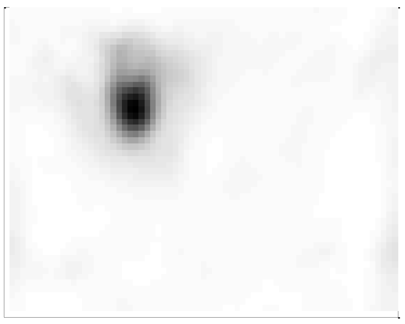
After pairing and scaling the mode shapes, the damage indices are computed following the procedure described in Section 2.2. The results are presented in Figure 18.
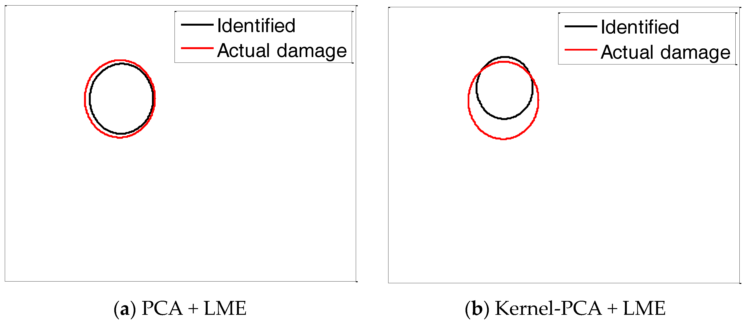
Figure 19 presents the damage assessment results obtained using PCA + LME and kernel-PCA + LME. Even though kernel-PCA + LME provided better results for the evaluation database, when working with experimental data PCA + LME outperformed it.
The localization and quantification errors are summarized in Table 2. The experimental errors for the PCA + LME are lower than the evaluation errors obtained in Section 5.1. This demonstrates that the proposed approach, trained with simulated numerical data, can be successfully used to assess experimental damage.
6. Concluding Remarks
A damage assessment algorithm that uses damage indices derived from the modal strain energy method and a linear approximation with maximum entropy algorithm has been implemented to assess debonding damage in honeycomb sandwich panels. Full-field vibration measurements of the panels have been acquired by a high-speed 3D digital image correlation (DIC) system. Two data reduction schemes have been implemented: PCA and kernel PCA.
The numerical results show that both algorithms have similar results, with kernel-PCA + LME performing slightly better for small damage. In addition, it can be concluded that, for the panel under investigation, when the normalized damage size is larger than 0.1, both algorithms locate and quantify the damage with precision. For normalized damage sizes between 0.025 and 0.1, it is possible to correctly quantify the damage and to provide an estimation of its location, and for normalized damage sizes smaller than 0.025, quantification is not possible.
The best experimental damage assessment results are obtained with the combination of PCA and LME algorithms. The experimental damaged region has been precisely localized and quantified. Therefore, the proposed methodology can be used successfully to identify debonding in composite panels.
It should be noted that the proposed methodology can be implemented with damage indices derived from any methodology. Therefore, a topic of further research is to evaluate if the performance of the proposed approach can be improved by using damage indices computed from other methodologies available in literature such as mode shape curvatures, uniform load surface, gapped smoothing method, wavelet-based and others. In addition, further research is needed to adapt this algorithm to cases with multiple debonded regions and to test its performance in more realistic configurations than a free plate.
Acknowledgments
The authors acknowledge the partial financial support of the Chilean National Fund for Scientific and Technological Development (FONDECYT) under Grant No. 1170535 and the FONDEQUIP Program under grant EQM130026.
Author Contributions
Viviana Meruane designed the experiment, processed and analyzed the experimental data, and implemented the damage assessment algorithm. Matias Lasen investigated the application of different data reduction schemes and optimized algorithm performance. Alejandro Ortiz-Bernardin programmed the max-ent linear approximation algorithm and adapted it to the application case. Enrique López Droguett helped with the implementation of the principal component analysis. The article was written by Viviana Meruane, Matian Lasen, Alejandro Ortiz-Bernardin and Enrique López Droguett.
Conflicts of Interest
The authors declare no conflict of interest.
References
- Vinson, J.R. Sandwich structures: Past, present, and future. In Sandwich Structures 7: Advancing with Sandwich Structures and Materials; Springer: Dordrecht, The Netherlands, 2005; pp. 3–12. [Google Scholar]
- Herrmann, A.S.; Zahlen, P.C.; Zuardy, I. Sandwich Structures Technology in Commercail Aviation: Present Applications and Future Trends. In Sandwich Structures 7: Advancing with Sandwich Structures and Materials; Springer: Dordrecht, The Netherlands, 2005. [Google Scholar]
- Carden, E.; Fanning, P. Vibration based condition monitoring: A review. Struct. Health Monit. 2004, 3, 355–377. [Google Scholar] [CrossRef]
- Jiang, L.; Liew, K.; Lim, M.; Low, S. Vibratory behaviour of delaminated honeycomb structures: A 3-D finite element modelling. Comput. Struct. 1995, 55, 773–788. [Google Scholar] [CrossRef]
- Burlayenko, V.; Sadowski, T. Dynamic behaviour of sandwich plates containing single/multiple debonding. Comput. Mater. Sci. 2011, 50, 1263–1268. [Google Scholar] [CrossRef]
- Burlayenko, V.N.; Sadowski, T. Influence of skin/core debonding on free vibration behavior of foam and honeycomb cored sandwich plates. Int. J. Non-Linear Mech. 2010, 45, 959–968. [Google Scholar] [CrossRef]
- Kim, H.-Y.; Hwang, W. Effect of debonding on natural frequencies and frequency response functions of honeycomb sandwich beams. Compos. Struct. 2002, 55, 51–62. [Google Scholar] [CrossRef]
- Lou, J.; Wu, L.; Ma, L.; Xiong, J.; Wang, B. Effects of local damage on vibration characteristics of composite pyramidal truss core sandwich structure. Compos. Part B Eng. 2014, 62, 73–87. [Google Scholar] [CrossRef]
- Shahdin, A.; Morlier, J.; Gourinat, Y. Damage monitoring in sandwich beams by modal parameter shifts: A comparative study of burst random and sine dwell vibration testing. J. Sound Vib. 2010, 329, 566–584. [Google Scholar] [CrossRef] [Green Version]
- Farrar, C.R.; Lieven, N.A. Damage prognosis: The future of structural health monitoring. Philos. Trans. R. Soc. Lond. A Math. Phys. Eng. Sci. 2007, 365, 623–632. [Google Scholar] [CrossRef] [PubMed]
- Meruane, V.; del Fierro, V. An inverse parallel genetic algorithm for the identification of skin/core debonding in honeycomb aluminium panels. Struct. Control Health Monit. 2015, 22, 1426–1439. [Google Scholar] [CrossRef]
- Islam, A.S.; Craig, K.C. Damage detection in composite structures using piezoelectric materials (and neural net). Smart Mater. Struct. 1994, 3, 318–328. [Google Scholar] [CrossRef]
- Okafor, A.C.; Chandrashekhara, K.; Jiang, Y. Delamination prediction in composite beams with built-in piezoelectric devices using modal analysis and neural network. Smart Mater. Struct. 1996, 5, 338–347. [Google Scholar] [CrossRef]
- Valoor, M.T.; Chandrashekhara, K. A thick composite-beam model for delamination prediction by the use of neural networks. Compos. Sci. Technol. 2000, 60, 1773–1779. [Google Scholar] [CrossRef]
- Ishak, S.; Liu, G.; Shang, H.; Lim, S. Locating and sizing of delamination in composite laminates using computational and experimental methods. Compos. Part B Eng. 2001, 32, 287–298. [Google Scholar] [CrossRef]
- Chakraborty, D. Artificial neural network based delamination prediction in laminated composites. Mater. Des. 2005, 26, 1–7. [Google Scholar] [CrossRef]
- Su, Z.; Ling, H.-Y.; Zhou, L.-M.; Lau, K.-T.; Ye, L. Efficiency of genetic algorithms and artificial neural networks for evaluating delamination in composite structures using fibre Bragg grating sensors. Smart Mater. Struct. 2005, 14, 1541–1553. [Google Scholar] [CrossRef]
- Zhang, Z.; Zhan, C.; Shankar, K.; Morozov, E.V.; Singh, H.K.; Ray, T. Sensitivity analysis of inverse algorithms for damage detection in composites. Compos. Struct. 2017, 176, 844–859. [Google Scholar] [CrossRef]
- Zhang, Z.; Shankar, K.; Ray, T.; Morozov, E.V.; Tahtali, M. Vibration-based inverse algorithms for detection of delamination in composites. Compos. Struct. 2013, 102, 226–236. [Google Scholar] [CrossRef]
- Meruane, V.; Mahu, J. Real-time structural damage assessment using artificial neural networks and anti-resonant frequencies. Shock Vib. 2014, 2014, 653279. [Google Scholar]
- Meruane, V.; Ortiz-Bernardin, A. Structural damage assessment using linear approximation with maximum entropy and transmissibility dat. Mech. Syst. Signal Process. 2015, 54, 210–223. [Google Scholar] [CrossRef]
- Meruane, V.; del Fierro, V.; Ortiz-Bernardin, A. A Maximum Entropy Approach to Assess Debonding in Honeycomb Aluminum Plates. Entropy 2014, 16, 2869–2889. [Google Scholar] [CrossRef]
- Sanchez, N.; Meruane, V.; Ortiz-Bernardin, A. A novel impact identification algorithm based on a linear approximation with maximum entropy. Smart Mater. Struct. 2016, 25, 095050. [Google Scholar] [CrossRef]
- Meruane, V.; Véliz, P.; Droguett, E.L.; Ortiz-Bernardin, A. Impact Location and Quantification on an Aluminum Sandwich Panel Using Principal Component Analysis and Linear Approximation with Maximum Entropy. Entropy 2017, 19, 137. [Google Scholar] [CrossRef]
- Cawley, P.; Adams, R.D. The location of defects in structures from measurements of natural frequencies. J. Strain Anal. Eng. Des. 1979, 14, 49–57. [Google Scholar] [CrossRef]
- Lieven, N.A.J.; Ewins, D.J. Spatial correlation of mode shapes, the coordinate modal assurance criterion (COMAC). In Proceedings of the Sixth International Modal Analysis Conference, Orlando, FL, USA, 1–4 February 1988. [Google Scholar]
- Pandey, A.K.; Biswas, M.; Samman, M.M. Damage detection from changes in curvature mode shapes. J. Sound Vib. 1991, 145, 321–332. [Google Scholar] [CrossRef]
- Pandey, A.K.; Biswas, M. Damage detection in structures using changes in flexibility. J. Sound Vib. 1994, 169, 3–17. [Google Scholar] [CrossRef]
- Zhang, Z.; Aktan, A.E. Application of modal flexibility and its derivatives in structural identification. J. Res. Nondestruct. Eval. 1998, 10, 43–61. [Google Scholar] [CrossRef]
- Shi, Z.Y.; Law, S.S.; Zhang, L.M. Structural damage localization from modal strain energy change. J. Sound Vib. 1998, 218, 825–844. [Google Scholar] [CrossRef]
- Cornwell, P.; Doebling, S.W.; Farrar, C.R. Application of the strain energy damage detection method to plate-like structures. J. Sound Vib. 1999, 224, 359–374. [Google Scholar] [CrossRef]
- Li, Y.Y.; Cheng, L.; Yam, L.H.; Wong, W.O. Identification of damage locations for plate-like structures using damage sensitive indices: Strain modal approach. Comput. Struct. 2002, 80, 1881–1894. [Google Scholar] [CrossRef]
- Wu, D.; Law, S.S. Damage localization in plate structures from uniform load surface curvature. J. Sound Vib. 2004, 276, 227–244. [Google Scholar] [CrossRef]
- Wu, D.; Law, S.S. Sensitivity of uniform load surface curvature for damage identification in plate structures. Trans. ASME-J. Vib. Acoust. 2005, 127, 84–92. [Google Scholar] [CrossRef]
- Yoon, M.K.; Heider, D.; Gillespie, J.W.; Ratcliffe, C.P.; Crane, R.M. Local damage detection using the two-dimensional gapped smoothing method. J. Sound Vib. 2005, 279, 119–139. [Google Scholar] [CrossRef]
- Qiao, P.; Lu, K.; Lestari, W.; Wang, J. Curvature mode shape-based damage detection in composite laminated plates. Compos. Struct. 2007, 80, 409–428. [Google Scholar] [CrossRef]
- Moreno-García, P.; Lopes, H.; Santos, J.V.A.D.; Maia, N.M.M. Damage localisation in composite laminated plates using higher order spatial derivatives. In Proceedings of the Eleventh International Conference on Computational Structures Technology, Dubrovnik, Croatia, 4–7 September 2012. [Google Scholar]
- Chang, C.C.; Chen, L.W. Damage detection of a rectangular plate by spatial wavelet based approach. Appl. Acoust. 2004, 65, 819–832. [Google Scholar] [CrossRef]
- Douka, E.; Loutridis, S.; Trochidis, A. Crack identification in plates using wavelet analysis. J. Sound Vib. 2004, 270, 279–295. [Google Scholar] [CrossRef]
- Rucka, M.A.; Wilde, K.R. Application of continuous wavelet transform in vibration based damage detection method for beams and plates. J. Sound Vib. 2006, 297, 536–550. [Google Scholar] [CrossRef]
- Huang, Y.; Meyer, D.; Nemat-Nasser, S. Nemat-Nasser, Damage detection with spatially distributed 2D continuous wavelet transform. Mech. Mater. 2009, 41, 1096–1107. [Google Scholar] [CrossRef]
- Fan, W.; Qiao, P. A 2-D continuous wavelet transform of mode shape data for damage detection of plate structures. Int. J. Solids Struct. 2009, 46, 4379–4395. [Google Scholar] [CrossRef]
- Yang, C.; Oyadiji, S.O. Delamination detection in composite laminate plates using 2D wavelet analysis of modal frequency surface. Comput. Struct. 2017, 179, 109–126. [Google Scholar] [CrossRef]
- Katunin, A. Damage identification in composite plates using two-dimensional B-spline wavelets. Mech. Syst. Signal Process. 2011, 25, 3153–3167. [Google Scholar] [CrossRef]
- Katunin, A. Stone impact damage identification in composite plates using modal data and quincunx wavelet analysis. Arch. Civ. Mech. Eng. 2015, 15, 251–261. [Google Scholar] [CrossRef]
- Katunin, A. Vibration-based spatial damage identification in honeycomb-core sandwich composite structures using wavelet analysis. Compos. Struct. 2014, 118, 385–391. [Google Scholar] [CrossRef]
- Seguel, F. Identificación de daño en Placas tipo Sándwich Usando un Sistema de Correlación de Imágenes Digital y la Curvatura de los Modos de Vibración. Master’s Thesis, Universidad de Chile, Santiago, Chile, 2016. (In Spanish). [Google Scholar]
- Helfrick, M.N.; Niezrecki, C.; Avitabile, P.; Schmidt, T. 3D digital image correlation methods for full-field vibration measurement. Mech. Syst. Signal Process. 2011, 25, 917–927. [Google Scholar] [CrossRef]
- Castellini, P.; Revel, G. An experimental technique for structural diagnostic based on laser vibrometry and neural networks. Shock Vib. 2000, 7, 381–397. [Google Scholar] [CrossRef]
- Schölkopf, B.; Smola, A.; Müller, K.R. Kernel principal component analysis. In International Conference on Artificial Neural Networks; Springer: Berlin/Heidelberg, Germany, 1997. [Google Scholar]
- Wang, Q. Kernel principal component analysis and its applications in face recognition and active shape model. arXiv, 2012; arXiv:1207.3538. [Google Scholar]
- Devroye, L.; Gyorfi, L.; Krzyzak, A.; Lugosi, G. On the strong universal consistency of nearest neighbor regression function estimates. Ann. Stat. 1994, 1994, 1371–1385. [Google Scholar] [CrossRef]
- Gupta, M.R.; Gray, R.M.; Olshen, R.A. Nonparametric supervised learning by linear. IEEE Trans. Pattern Anal. Mach. 2006, 28, 766–781. [Google Scholar] [CrossRef] [PubMed]
- Sukumar, N.; Wright, R. Overview and construction of meshfree basis functions: From moving least squares to entropy approximants. Int. J. Numer. Methods Eng. 2007, 70, 181–205. [Google Scholar] [CrossRef]
- Siebert, T.; Becker, T.; Spiltthof, K.; Neumann, I.; Krupka, R. High-speed digital image correlation: Error estimations and applications. Opt. Eng. 2007, 46, 051004. [Google Scholar] [CrossRef]
- Siebert, T.; Wood, R.; Splitthof, K. High speed image correlation for vibration analysis. J. Phys. Conf. Ser. 2009, 181, 012064. [Google Scholar] [CrossRef]
- Balmes, E.; Bianchi, J.P.; Leclère, J.M. Structural Dynamics Toolbox Users Guide; Version 6.1; Scientific Software Group: Paris, France, 2009. [Google Scholar]
Figure 1.
Principle of a vibration-based damage assessment algorithm.

Figure 2.
Damage parameterization.
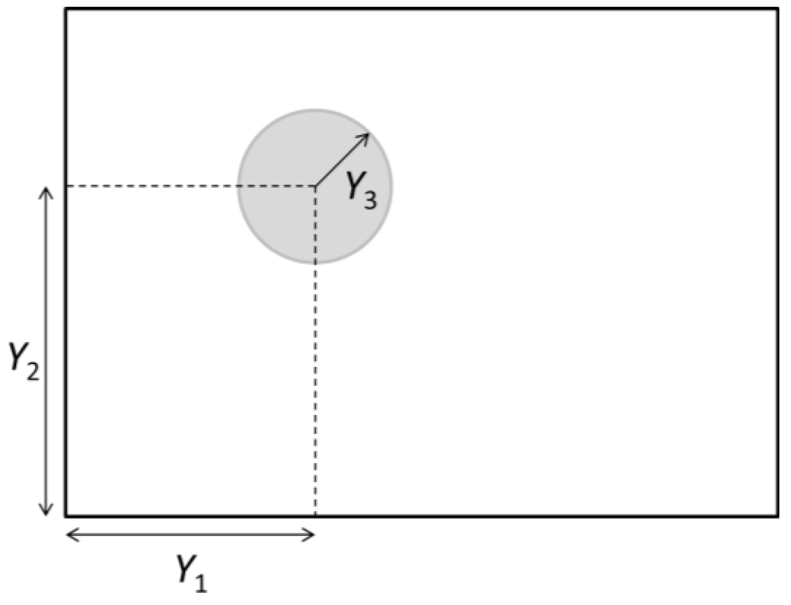
Figure 3.
Scheme of the experimental setup.

Figure 4.
Vibration measurements acquired with the high-speed 3D digital image correlation (DIC) system: (a) High-speed cameras aimed at the panel; (b) Vibration mode shape at 444 Hz.
Figure 4.
Vibration measurements acquired with the high-speed 3D digital image correlation (DIC) system: (a) High-speed cameras aimed at the panel; (b) Vibration mode shape at 444 Hz.
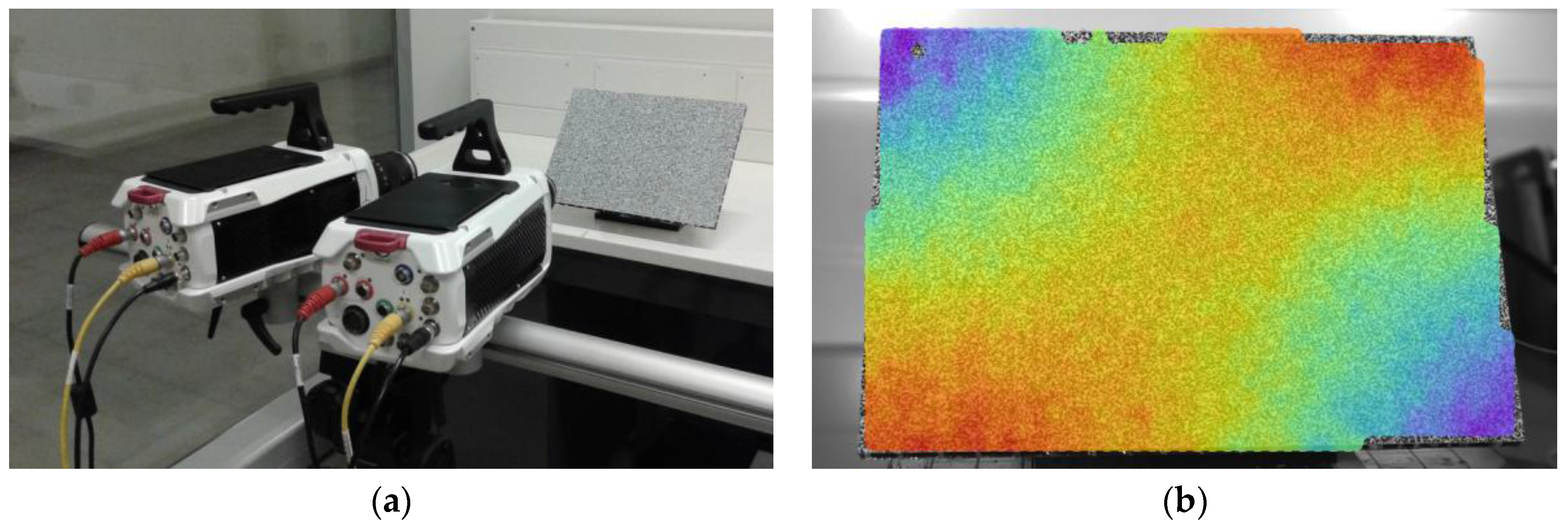
Figure 5.
Identified mode shapes for the undamaged case.
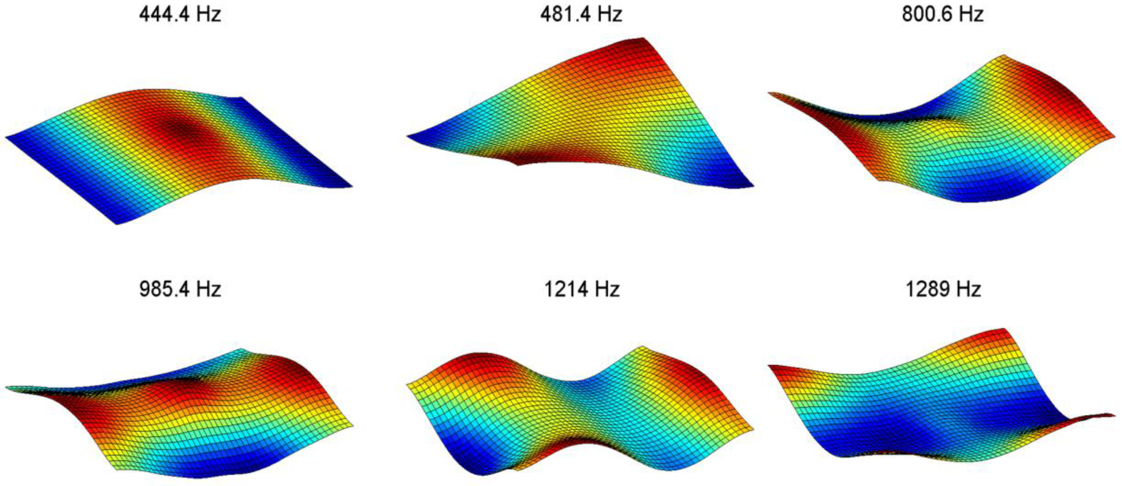
Figure 6.
Identified mode shapes for a debonded case.

Figure 7.
Lateral view of the numerical model: (a) undamaged panel; (b) panel with a debonded region.
Figure 7.
Lateral view of the numerical model: (a) undamaged panel; (b) panel with a debonded region.

Figure 8.
Distribution of damage indices obtained for three different damage scenarios.
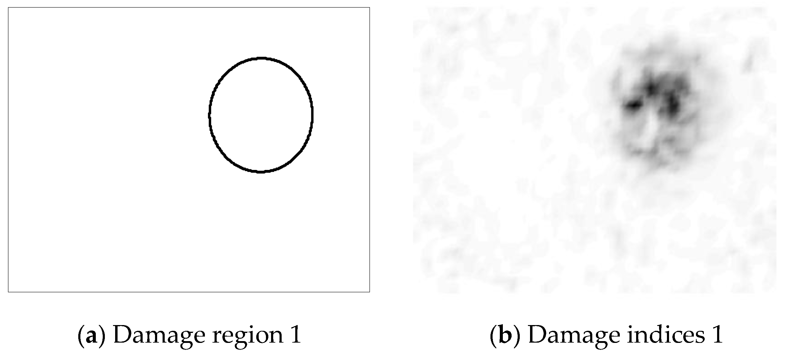

Figure 9.
Localization and quantification errors obtained for different combinations of the parameters n and k.
Figure 9.
Localization and quantification errors obtained for different combinations of the parameters n and k.
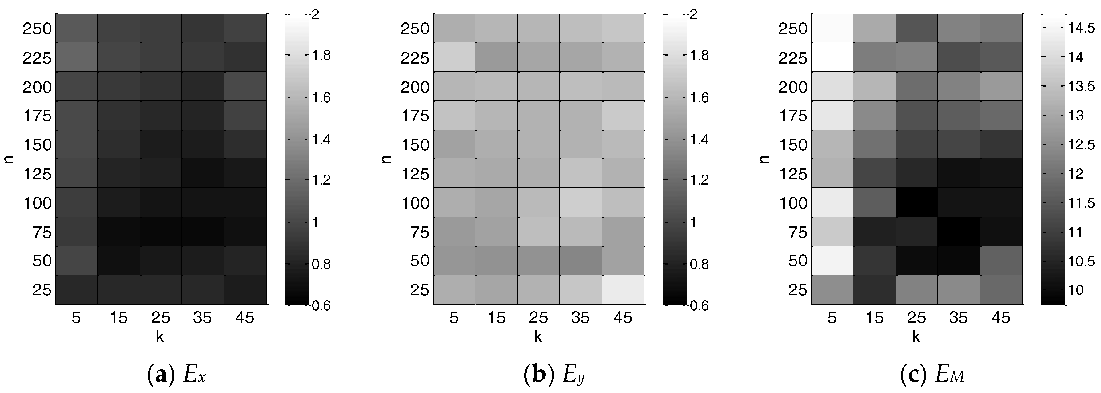
Figure 10.
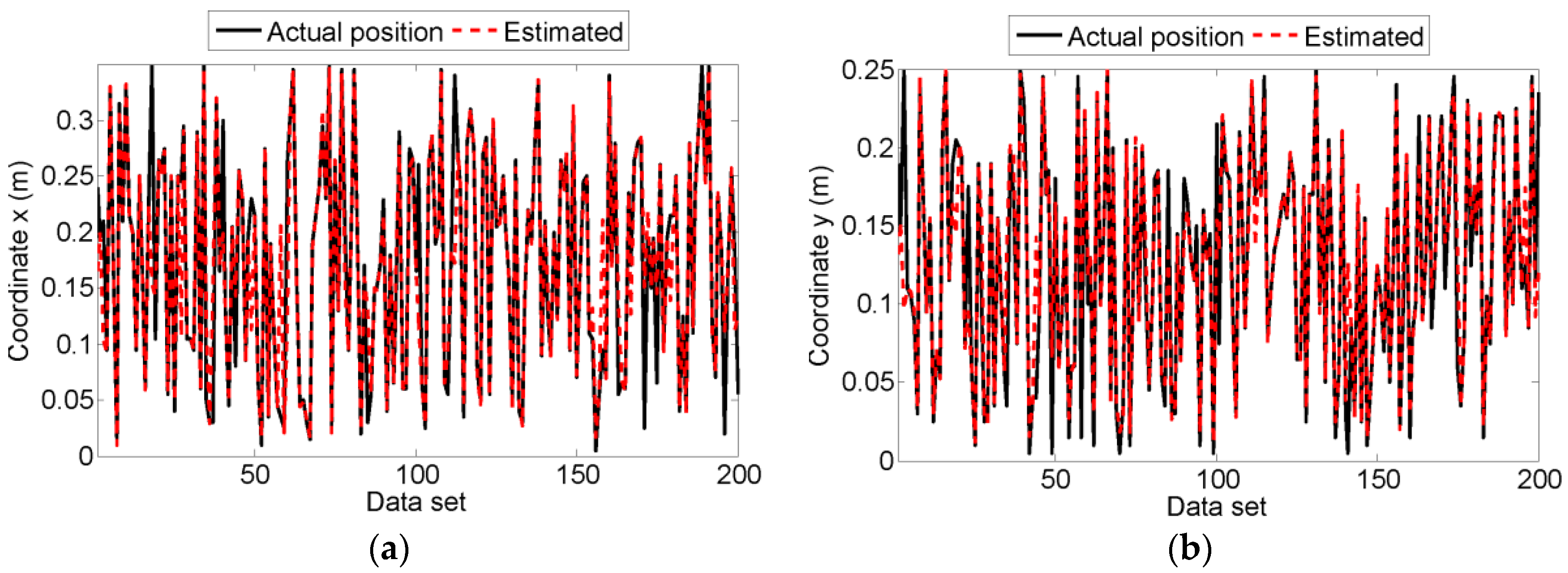
Damage localization results using principal component analysis (PCA) + linear approximation with maximum entropy (LME) and the evaluation database.
Figure 10.
Damage localization results using principal component analysis (PCA) + linear approximation with maximum entropy (LME) and the evaluation database.
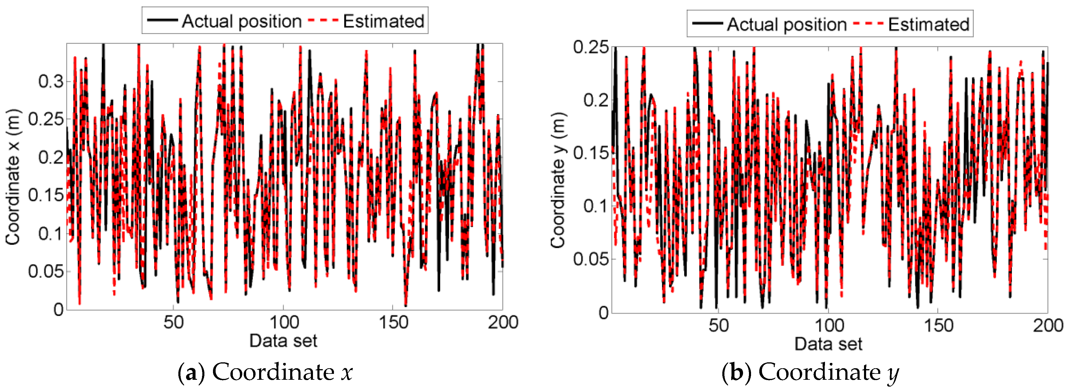
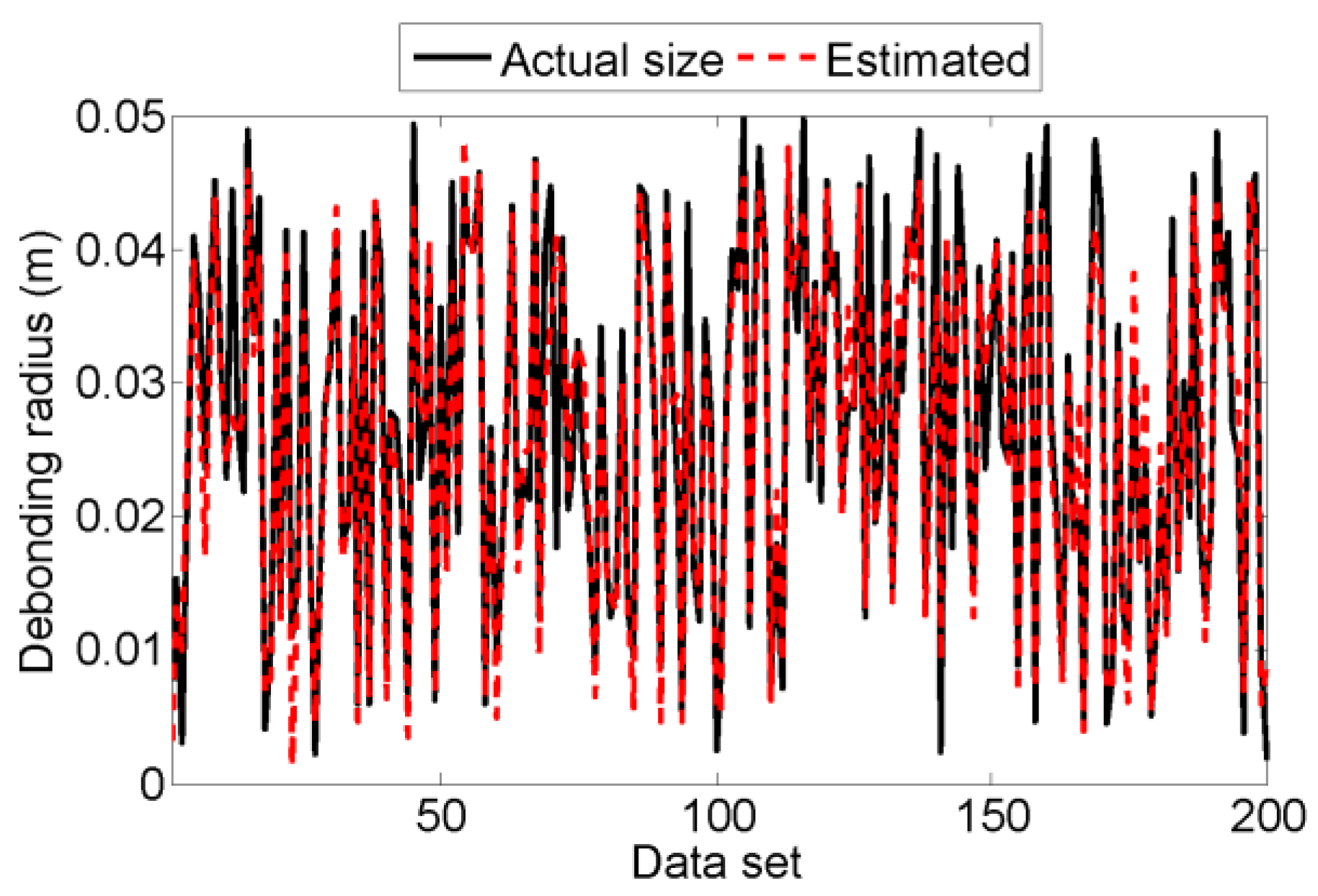
Figure 11.
Damage quantification results using PCA + LME and the evaluation database.

Figure 12.
Localization and quantification errors obtained for different combinations of the parameters n and σ.
Figure 12.
Localization and quantification errors obtained for different combinations of the parameters n and σ.

Figure 13.
Damage localization results using kernel-PCA + LME and the evaluation database.

Figure 14.
Damage quantification results using kernel-PCA + LME and the evaluation database.
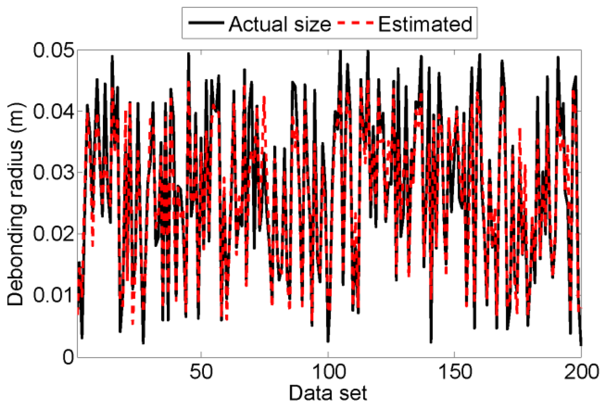
Figure 15.
Damage localization error as a function of the normalized damage size.
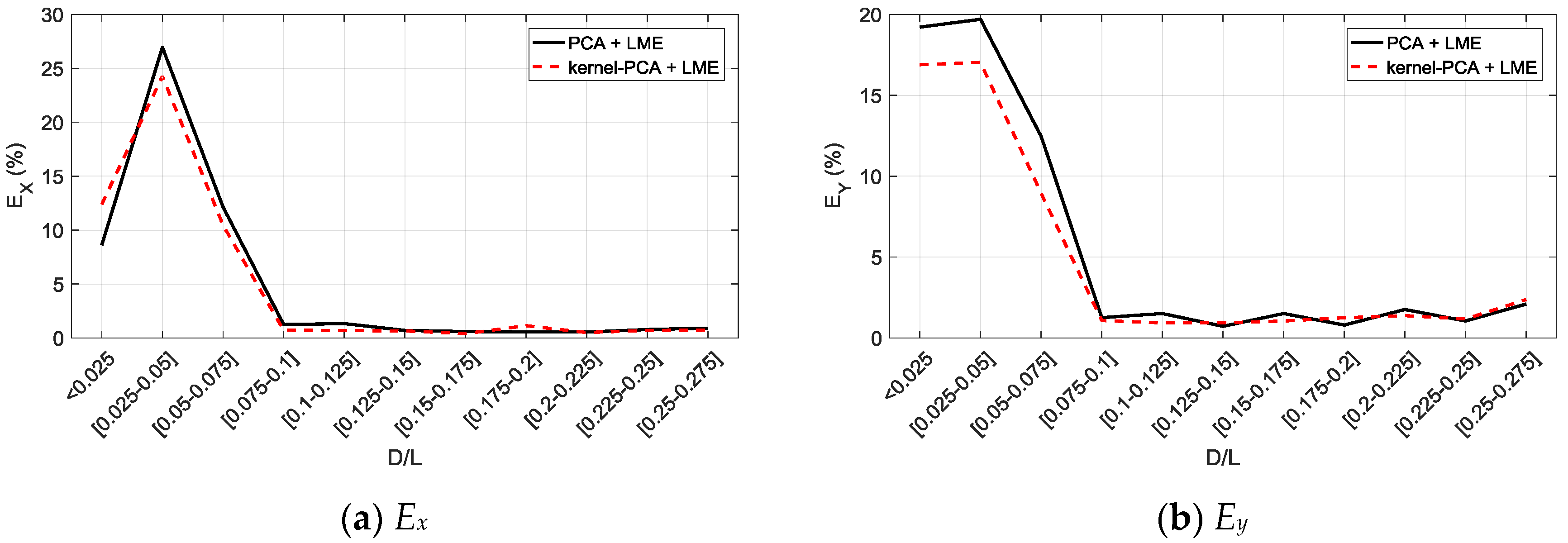
Figure 16.
Damage quantification error as a function of the normalized damage size.
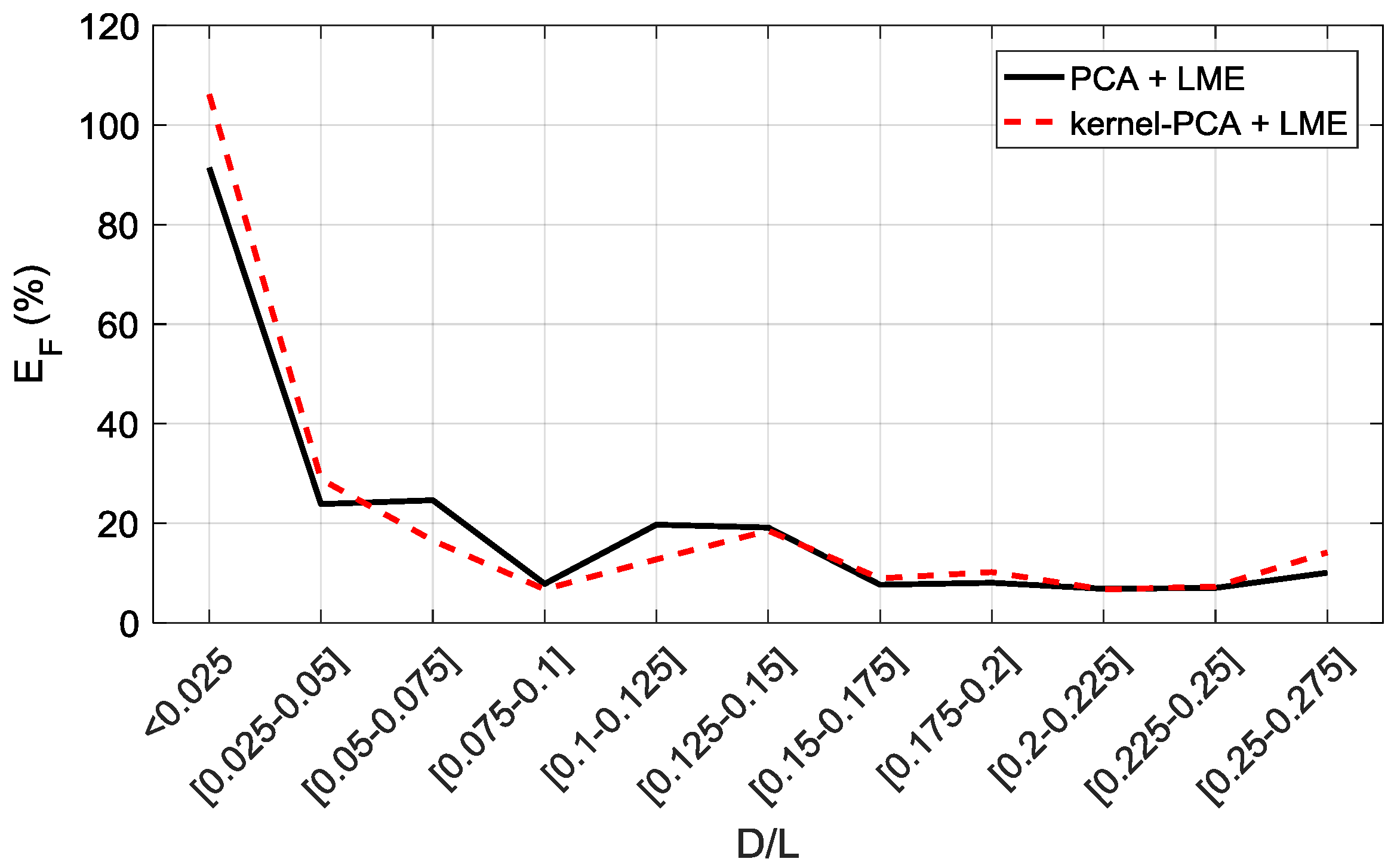
Figure 17.
Experimental damage introduced to the panel; the red line indicates the debonded region.
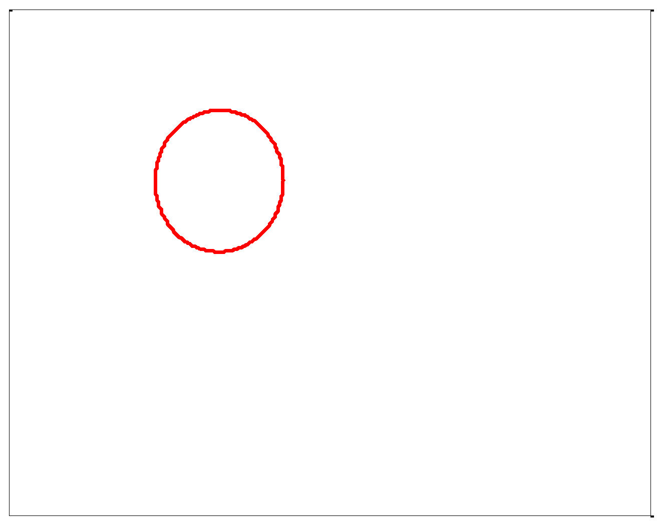
Figure 18.
Distribution of experimental damage indices.

Figure 19.
Experimental damage assessment results.

Table 1.
Pairs of undamaged and damaged mode shapes. MAC: modal assurance criterion.
| Mode Shape Pair | (Hz) | (Hz) | (%) | MAC |
|---|---|---|---|---|
| 1 | 444 | 440 | –0.9 | 0.97 |
| 2 | 481 | 493 | 2.5 | 0.90 |
| 3 | 801 | 798 | –0.4 | 0.98 |
| 4 | 985 | 820 | –16.8 | 0.68 |
| 5 | 1290 | 1230 | –4.7 | 0.67 |
Table 2.
Damage localization and quantification errors.
| PCA + LME | Kernel PCA + LME | |
|---|---|---|
| (%) | 0.46 | 0.36 |
| (%) | 0.03 | 4.43 |
| (%) | 9.59 | 19.90 |
© 2017 by the authors. Licensee MDPI, Basel, Switzerland. This article is an open access article distributed under the terms and conditions of the Creative Commons Attribution (CC BY) license (http://creativecommons.org/licenses/by/4.0/).
Share and Cite
MDPI and ACS Style
Meruane, V.; Lasen, M.; López Droguett, E.; Ortiz-Bernardin, A. Modal Strain Energy-Based Debonding Assessment of Sandwich Panels Using a Linear Approximation with Maximum Entropy. Entropy 2017, 19, 619. https://doi.org/10.3390/e19110619
AMA Style
Meruane V, Lasen M, López Droguett E, Ortiz-Bernardin A. Modal Strain Energy-Based Debonding Assessment of Sandwich Panels Using a Linear Approximation with Maximum Entropy. Entropy. 2017; 19(11):619. https://doi.org/10.3390/e19110619
Chicago/Turabian StyleMeruane, Viviana, Matias Lasen, Enrique López Droguett, and Alejandro Ortiz-Bernardin. 2017. "Modal Strain Energy-Based Debonding Assessment of Sandwich Panels Using a Linear Approximation with Maximum Entropy" Entropy 19, no. 11: 619. https://doi.org/10.3390/e19110619
Note that from the first issue of 2016, this journal uses article numbers instead of page numbers. See further details here.