Dynamic and Thermodynamic Properties of a CA Engine with Non-Instantaneous Adiabats
by
Ricardo T. Paéz-Hernández
1, 
Norma Sánchez-Salas
2,*,
Juan C. Chimal-Eguía
3 and
Delfino Ladino-Luna
1 1
Área de Física de Procesos Irreversibles, Departamento de Ciencias Básicas, Universidad Autónoma Metropolitana, U-Azcapotzalco, Av. San Pablo 180, col. Reynosa, CP 02200 Ciudad de México, Mexico
2
Departamento de Física, Escuela Superior de Física y Matemáticas, Instituto Politécnico Nacional, UP Zacatenco, CP 07738 Ciudad de México, Mexico
3
Laboratorio de Simulación y Modelado, Centro de Investigación en Computación, Instituto Politécnico Nacional, Av. Juan de Dios Batiz s/n UP Zacatenco, CP 07738 Ciudad de México, Mexico
*
Author to whom correspondence should be addressed.
Entropy 2017, 19(11), 632; https://doi.org/10.3390/e19110632
Submission received: 24 October 2017
/
Revised: 15 November 2017
/
Accepted: 17 November 2017
/
Published: 22 November 2017
(This article belongs to the Section Thermodynamics)
Abstract
:This paper presents an analysis of a Curzon and Alhborn thermal engine model where both internal irreversibilities and non-instantaneous adiabatic branches are considered, operating with maximum ecological function and maximum power output regimes. Its thermodynamic properties are shown, and an analysis of its local dynamic stability is performed. The results derived are compared throughout the work with the results obtained previously for a case in which the adiabatic branches were assumed as instantaneous. The results indicate a better performance for thermodynamic properties in the model with instantaneous adiabatic branches, whereas there is an improvement in robustness in the case where non-instantaneous adiabatic branches are considered.
1. Introduction
In the past 40 years, a branch of thermodynamics called finite-time thermodynamics (FTT) has been developed, based mainly on the pioneering work of Curzon and Ahlborn (CA) [1], although Novikov and Chambadal [2,3] had previously reported an equivalent analysis. CA formulated an engine with a modified Carnot cycle and proposed the so-called endoreversible hypothesis [4]. Its assignment has been applied for the analysis of several thermal heat engine models [5,6]. This hypothesis assumes that all irreversibilities in a thermal engine can be described only by the couplings between the working fluid and its environment, allowing the working substance to carry out reversible inner cycles. A more realistic case, which is therefore important to consider, is to include in the model both external and internal dissipations, since the internal dissipations also influence the performance of a thermal engine. Such irreversibilities are of major importance and some authors [7,8,9] have made contributions to the thermodynamic analysis of the CA engine. They proposed equivalent approaches for irreversible finite time thermodynamics, avoiding the endoreversible hypothesis defining a parameter R; all internal irreversibilities are included and when , the endoreversible model is recovered. In the context of FTT, several objective functions have been proposed. CA performed the analysis considering the maximum power output, and subsequently other criteria were presented. One of the criteria is the function known as ecological, introduced by Angulo–Brown [10]. For this criterion the value to maximize is a function that represents a trade-off between high power output and low entropy production defined as , where P represents the power output, the entropy production, and the cold thermal reservoir.
As is usual in FTT models the adiabatic branches are taken as instantaneous processes, i.e., the internal relaxation times in these branches are considered to be extremely short compared to the duration of the process [4]. Therefore, the cycle period is dominated by the isothermal branch times.
However, some other authors [11] have considered it important to take into account the time for all the cycle branches. For instance, Gutkowics–Krusin et al. [12] have shown that the CA efficiency is an upper bound for the efficiency as a function of both the ratio and the ratio of the maximum and the minimum volume spanned by the cycle, through the quantity with a maximum power regime using an ideal gas as a working substance. Later, Ladino–Luna et al. [13] also showed similar results for the model operating under an ecological criterion. Additionally, the authors studied the thermodynamical properties of a Curzon and Ahlborn engine when it takes into account the time for all the cycle branches and the Van der Waals gas as the working substance [14]. On the other hand, the effect of considering instantaneous and non-instantaneous adiabatic transitions has been analyzed for systems with micro- and nanometer-length scales [15,16,17].
While the vision of FTT was based on the study of optimal thermodynamic properties, Santillán et al. [18] changed the way of analysis for thermodynamic properties and introduced a novel manner to contextualize a heat engine based only on its thermodynamic properties, instead of its dynamic properties, in order to achieve a good engine design. Therefore, there arose two principles of robust design for heat engines, namely: (1) optimal thermodynamic properties; and (2) dynamical robustness of the system.
The second principle showed the important fact that the system stability should be allowed to maintain all of its operation in an internal or external regime despite the perturbations that may occur. On the other hand, the optimal thermodynamic properties, namely, high power output, high efficiency, low entropy production, etc., guarantee the convenience of the energy converting system.
Moreover, it has been shown [18,19,20,21,22,23] that these two physical properties inherently contain a certain kind of trade-off due to the fact that both are governed by the same parameters. The former reflects a certainty that while the stability becomes stronger the thermodynamic properties become weaker, and thus, it is clear that both properties must be adjusted in order to have the best possible system design. In this paper, the influence of considering non-instantaneous adiabatic branches in a CA engine with internal irreversibilities is presented. A comparison with the instantaneous adiabats case is made when the engine operates in two regimes: maximum power, and maximum ecological function. Section 2 presents the model and its thermodynamic performance for different cases. Section 3 gives the elements to perform a local stability analysis of the model and the details are provided for the ecological regime. In Section 4, the relaxation times for each of the cases of interest in this work are provided. Finally, in Section 5 some conclusions are given.
2. Thermal Properties of CA Engine with Internal Irreversibilities
In this section we summarize some features of a CA engine model with internal irreversibilities, considering two cases: with instantaneous adiabatic branches (IA), and with non-instantaneous adiabatic branches (NIA) in the cycle. A diagram of the engine is shown in Figure 1a, indicating external irreversibilities arising via the heat exchange between the thermal reservoirs and the effective temperature for working fluid, as well as internal irreversibilities, included by the irreversibility parameter R, with and where corresponds to the endoreversible CA engine [4]. Figure 1b is its corresponding T-S diagram.
It is possible to consider different types of heat transfer laws [24] with respect to the thermal reservoirs and the working fluid. In this work, only a linear heat transfer law is considered. The more extensively analyzed case is where instant adiabatic branches are assumed. Now, the thermodynamic properties for the model in the two optimal regimes of maximum power and ecological function are shown.
2.1. Maximum Power Output (MP)
In this regime, thermodynamic functions of the CA engine model with internal irreversibilities and instantaneous adiabatic branches [8,25] are given by
and
which are the power and the efficiency, respectively.
While non-instantaneous adiabatic branches are considered using an ideal gas as the working substance, in the linear approximation [26] it is possible to find the thermal properties
and
for the power and efficiency, respectively. These expressions are in accordance with the results reported in [27] when , and also with NIA conditions at maximum power output.
Figure 2a shows the behavior of the power output (Equations (1) and (3)), for two values of the parameter of irreversibility R. It can be observed that while R decreases, that is, internal irreversibilities increase, the power decreases. An equivalent performance can be seen for the efficiency in Equations (2) and (4), and Figure 2b displays the behavior. It is worth mentioning some characteristics of the optimal behavior of the thermodynamic properties. The values of both power and efficiency in the maximum power regime have higher values for the case in which instantaneous adiabats are considered than for non-instantaneous adiabats. Also, thermodynamic functions are constrained by the value of R. Both the power and the efficiency become zero at , and when the efficiency becomes negative in both IA [25] and NIA circumstances .
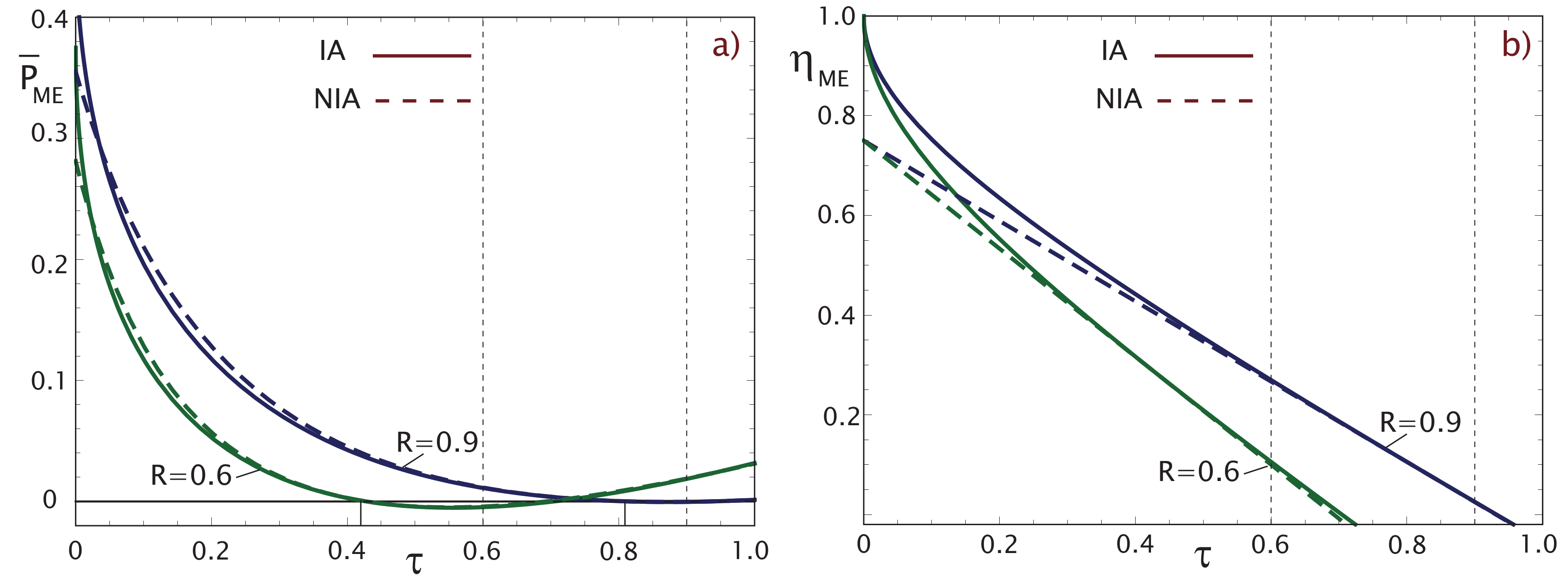
2.2. Maximum Ecological Criterion (ME)
As mentioned in the introduction, the ecological function proposed by Angulo–Brown [10] defined as , represents a trade-off between high power output and low entropy production. When the CA thermal engine operates under conditions of maximum ecological function considering internal irreversibilities and instantaneous adiabats, its power and efficiency are given by
and
When non-instantaneous adiabats are considered, in the linear approximation [26] in this regime, the following expressions are found,
which correspond to the power and efficiency, respectively. From Equation (8), when it follows that , as was previously reported [28].
The behavior of the optimized thermodynamic functions in this regime is shown in Figure 3. The power, as shown through Equations (5) and (7), is plotted for and in Figure 3a. As can be seen, the values for the power are practically the same in both the cases with IA and with NIA. This is a consequence of the fact that expression (7) with NIA has been obtained under an approximation. It can also be observed that a decrease of the parameter R, that is, an increase of the internal irreversibilities, causes a decrease of the power, as expected. A difference with the maximum power regime is that, in this case, the values of are more restricted, as , otherwise the power is negative. Figure 3b shows the behavior of optimal efficiency; it is greater when no instantaneous adiabats are considered. In the same way for greater internal irreversibilities, when R is lower, the efficiencies decrease. In summary, the CA engine with internal irreversibilities has a better thermodynamical performance when considering instantaneous adiabatic branches.
3. Steady-State Properties and Stability Analysis of the CA Engine
In this section the elements of the model in the steady state are presented in order to later perform a local stability analysis. The thermal engine operates between two thermal reservoirs at hot and cold temperatures, and , respectively, along a Carnot-like cycle composed of an irreversible internal part while also making irreversible heat exchanges with the temperature reservoirs. Figure 4 shows a diagram of the model. In the steady state the cycle temperatures in the isothermal branches are and , where (overbars indicate the corresponding steady-state variables). The heat flowing from the hot and to the cold thermal reservoirs in the steady state is denoted by and , respectively,
The inner part of the engine works in irreversible cycles, and from the Clausius theorem it follows that
The expression could be re-written as
where is the parameter of internal irreversibility.
The power output in the steady state can be expressed as
and the efficiency as,
In order to continue with the stability analysis, different scenarios for the operation of the engine are possible depending on the characteristics of the CA engine model and on the operating regime. In the previous section the thermodynamic performance of four cases was presented. The first was a model with internal irreversibilities operating at maximum power (Equations (1) and (2)). Paez et al. [25] presented the stability analysis of this case, so the details are not presented here, and the results will be given for comparison purposes. The second case was a model with internal irreversibilities and non-instantaneous adiabatic branches, using an ideal gas as a working substance in the regime of maximum power as shown in Equations (3) and (4). In this scenario, a stability study for a particular case when was presented in [27]. The third case [23] presented the stability analysis for an engine with internal irreversibilities operating at maximum ecological function (Equations (5) and (6)). The last case was a stability analysis where internal irreversibilities and non-instantaneous adiabats were included in the regime of the ecological function as detailed below.
The efficiency for the CA engine with internal irreversibilities in NIA conditions working in an ME regime using a linear approximation has been deduced from [26]
Finally, substituting (20) and (21) into (22) we get in terms of and . Notice and are not independent variables. Instead, their values are determined by the temperatures and and by the choice of the performance regime. Then
This expression corresponds to the power output in the ecological regime with both internal irreversibilities and non-instantaneous adiabats.
Dynamic Equations and Local Stability Analysis
Now, consider the CA engine of Figure 4, but out of the steady state, since x and y are not real heat reservoirs but macroscopic objects with heat capacity C. Their temperatures change following these differential equations:
Equation (13) represents the first law of thermodynamics and (14) is the definition of efficiency, so that they can be assumed to be valid even out of the steady state. Meanwhile in (12), the parameter R includes internal irreversibilities. It will be considered that it is also valid in the first approach outside the steady state. By making these considerations it is possible to write the following expressions for and :
Similarly, we consider that the power P obtained out of the steady state, but not so far away, depends on x and y in the same way that depends on and in the steady state, namely, ,18] so that
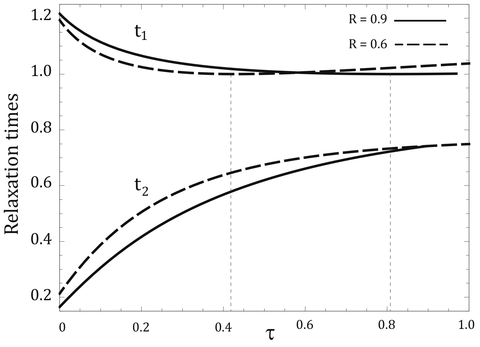
From the dynamic non-linear Equations (24) and (25), we followed a well-known procedure to analyze the local stability of a system using the linearization technique [29]. The above provides us with information about the qualitative behavior of the phase portrait for the system near the fixed point. The Jacobian matrix J is determined and its eigenvalues, and , are found. Since both are negative real numbers this implies that the system steady state is a stable node and allows us to define the relaxation times as , . Figure 5 shows the behavior of relaxation times as functions of for two values of parameter R in the ME regime with NIA branches.
From this figure it is possible to conclude that the increase of and decline of R improves the system stability within the range of validity of for each corresponding value of R. We remember in this regime that its values are more restricted than in the maximum power case.
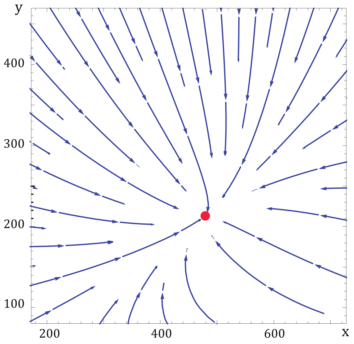
In order to acquire more information about system stability, in Figure 6 a plot of the velocity vector field is presented which is consistent with the relaxation times (Figure 5) obtained with the approximate analysis using the linearization technique. Although parameter values would be changed, the qualitative features are maintained.
4. Relaxation Times for NI and NIA Adiabats: A Comparative Analysis
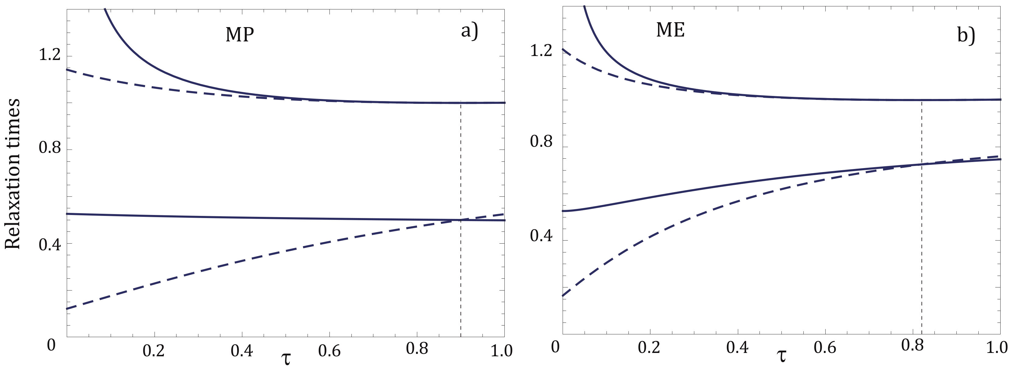
In this section we present a comparative analysis of the local dynamic stability for the CA engine model where internal irreversibilities are considered for both the instantaneous and non-instantaneous adiabatic branches case, operating with two regimes: maximum power, and maximum ecological function. Specifically, the relaxation time evolution derived from the linearization of the dynamic equations [23,25,27,29] are shown. Figure 7 shows the behavior of the relaxation times for the CA engine operating at maximum power (a) and maximum ecological function (b). Internal irreversibilities are considered since . The solid lines correspond to the case in which the instantaneous adiabats are taken and the dashed lines correspond to the case with non-instantaneous adiabats. From the plot it is observed that considering non-instantaneous adiabats reduces the relaxation times and therefore it can be considered that this increases the CA engine robustness.
5. Concluding Remarks
In this work the performance of the CA engine with internal irreversibilities considering instantaneous and non-instantaneous adiabatic branches is shown, operating with two regimes: MP and ME. Section 2 presented the behavior of its thermodynamic properties and it was found that the engine has better properties when the adiabatic branches are instantaneous for the MP case, and for ME the improvement is not noticeable. As has been mentioned in previous works, the optimum efficiency of the ME regime is greater than of the MP regime. In both MP and ME, the range is restricted by the value of R, and R decreases, reducing the performance of the thermodynamic functions engine. The analysis of the local stability for the engine was detailed considering non-instantaneous adiabats in the ME regime that had not been previously presented, with the following results. The model is stable with a fixed point, and remains so when the irreversibilities increase. That is, R decreases the CA engine, reducing its relaxation times and therefore increasing its stability. Finally, we show the relaxation times for the model considering internal irreversibilities with instantaneous and non-instantaneous adiabatic branches operating at MP and ME. It is possible to observe the effect on the model when comparing the IA and the NIA case. The analysis shows that consideration of NIA branches gives the system more robustness.
Acknowledgments
This research was partially supported by the Consejo Nacional de Ciencia y Tecnología (CONACyT, Mexico). NSS and JCCE also give thanks to COFAA-IPN and EDI-IPN.
Author Contributions
All authors made substantial contributions to the analysis and conclusions presented in this work. All authors have read and approved the final manuscript.
Conflicts of Interest
The authors declare no conflict of interest.
References
- Curzon, F.L.; Ahlborn, B. Efficiency of a Carnot Engine at Maximum Power Output. Am. J. Phys. 1975, 43, 22–24. [Google Scholar] [CrossRef]
- Novikov, I.I. The efficiency of atomic power stations (a review). J. Nucl. Energy 1958, 7, 125–128. [Google Scholar] [CrossRef]
- Chambadal, P. Les Centrales Nuclaires; Armand Colin: Paris, France, 1957. (In French) [Google Scholar]
- Rubin, M.H. Optimal configuration of a class of irreversible heat engines. I. Phys. Rev. A 1979, 19, 1272–1276. [Google Scholar] [CrossRef]
- Berry, R.S.; Kazakov, V.A.; Sieniutycz, S.; Szwast, Z.; Tsirlin, A.M. Thermodynamics Optimization of Finite-Time Processes; John Wiley and Sons: New York, NY, USA, 2000. [Google Scholar]
- Chen, L.; Sun, F. Advances in Finite Time Thermodynamics: Analysis and Optimization; Nova Science Publisher: New York, NY, USA, 2004. [Google Scholar]
- Ozkaynak, S.; Gokun, S.; Yavuz, H. Finite-time thermodynamic analysis of a radiative heat engine with internal irreversibility. J. Phys. D Appl. Phys. 1994, 27, 1139–1143. [Google Scholar] [CrossRef]
- Chen, J. The maximum power output and maximum efficiency of an irreversible Carnot heat engine. J. Phys. D Appl. Phys. 1994, 27, 1144–1149. [Google Scholar]
- Feidt, M.; Costea, M.; Petrescu, S.; Stanciu, C. Nonlinear Thermodynamic Analysis and Optimization of a Carnot Engine Cycle. Entropy 2016, 18, 243. [Google Scholar] [CrossRef]
- Angulo-Brown, F. An ecological optimization criterion for finite-time heat engines. J. Appl. Phys. 1991, 69, 7465–7469. [Google Scholar] [CrossRef]
- Agrawal, D.C.; Gordon, J.M.; Huleihil, M. Endoreversible engines with finite-time adiabats. Indian J. Eng. Mater. Sci. 1994, 1, 195–198. [Google Scholar]
- Gutkowicz-Krusin, D.; Procaccia, I.; Ross, J. On the efficiency of rate processes. Power and efficiency of heat engines. J. Chem. Phys. 1978, 69, 3898–3906. [Google Scholar] [CrossRef]
- Ladino-Luna, D.; de la Selva, S.T. The ecological efficiency of a thermal finite time engine. Rev. Mex. Fís. 2000, 46, 52–56. [Google Scholar]
- Ladino-Luna, D. Van der Waals gas as working substance in a Curzon and Ahlborn-Novikov engine. Entropy 2005, 7, 108–121. [Google Scholar] [CrossRef]
- Martínez, I.A.; Roldán, E.; Dinis, L.; Petrov, D.; Rica, R.A. Adiabatic Processes Realized with a Trapped Brownian Particle. Phys. Rev. Lett. 2015, 114, 120601. [Google Scholar] [CrossRef] [PubMed]
- Martínez, I.A.; Roldán, E.; Dinis, L.; Rica, R.A. Colloidal heat engines: A review. Soft Matter 2017, 13, 22–36. [Google Scholar] [CrossRef] [PubMed]
- Blickle, V.; Bechinger, C. Realization of a micrometre-sized stochastic heat engine. Nat. Phys. 2012, 8, 143–146. [Google Scholar] [CrossRef]
- Santillán, M.; Maya, G.; Angulo-Brown, F. Local stability analysis of an endoreversible Curzon-Ahborn-Novikov engine working in a maximum-power-like regime. J. Phys. D Appl. Phys. 2001, 34, 2068–2072. [Google Scholar] [CrossRef]
- Guzmán-Vargas, L.; Reyes-Ramírez, I.; Sánchez, N. The effect of heat transfer laws and thermal conductances on the local stability of an endoreversible heat engine. J. Phys. D Appl. Phys. 2005, 38, 1282–1291. [Google Scholar] [CrossRef]
- Chimal-Eguía, J.C.; Barranco-Jiménez, M.A.; Angulo-Brown, F. Stability Analysis of an Endoreversible Heat Engine with Stefan-Boltzmann Heat Transfer Law Working in Maximum-Power-Like Regime. Open Syst. Inf. Dyn. 2006, 13, 43–53. [Google Scholar] [CrossRef]
- Nie, W.; He, J.; Deng, X. Local stability analysis of an irreversible Carnot heat engine. Int. J. Therm. Sci. 2008, 47, 633–640. [Google Scholar] [CrossRef]
- Huang, Y.; Sun, D.; Kang, Y. Local stability characteristics of a non-endoreversible heat engine working in the optimum region. Appl. Therm. Eng. 2009, 29, 358–363. [Google Scholar] [CrossRef]
- Sanchez-Salas, N.; Chimal-Eguia, J.C.; Guzman-Aguilar, F. On the Dynamic Robustness of a Non-Endoreversible Engine Working in Different Operation Regimes. Entropy 2011, 13, 422–436. [Google Scholar] [CrossRef]
- Chen, L.; Yan, Z. The effect of heat-transfer law on performance of a two-heat-source endoreversible cycle. J. Chem. Phys. 1989, 90, 3740–3743. [Google Scholar] [CrossRef]
- Páez-Hernández, R.; Angulo-Brown, F.; Santillán, M. Dynamic Robustness and Thermodynamic Optimization in a Non-Endoreversible Curzon-Ahlborn Engine. J. Non-Equilib. Thermodyn. 2006, 31, 173–188. [Google Scholar]
- Ladino-Luna, D. Linear approximation of efficiency for a non-endoreversible cycle. J. Energy Inst. 2011, 84, 61–65. [Google Scholar] [CrossRef]
- Páez-Hernández, R.; Ladino-Luna, D.; Portillo-Díaz, P. Dynamic properties in an endoreversible Curzon-Ahlborn engine using a van der Waals gas as working substance. Phys. A Stat. Mech. Appl. 2011, 390, 3275–3282. [Google Scholar] [CrossRef]
- Páez-Hernández, R.; Ladino-Luna, D.; Portillo-Díaz, P.; Barranco-Jiménez, M. Local Stability Analysis of a Curzon-Ahlborn Engine without Ideal Gas Working at the Maximum Ecological Regime. J. Energy Power Eng. 2013, 7, 928–936. [Google Scholar]
- Strogatz, S.H. Nonlinear Dynamics and Chaos: With Applications to Physics, Biology, Chemistry, and Engineering; Westview Press: Boulder, CO, USA, 2001. [Google Scholar]
Figure 1.
(a) Diagram of Curzon and Ahlborn engine where both internal and external irreversibilities are considered; and (b) the corresponding T-S diagram of the cycle.
Figure 1.
(a) Diagram of Curzon and Ahlborn engine where both internal and external irreversibilities are considered; and (b) the corresponding T-S diagram of the cycle.
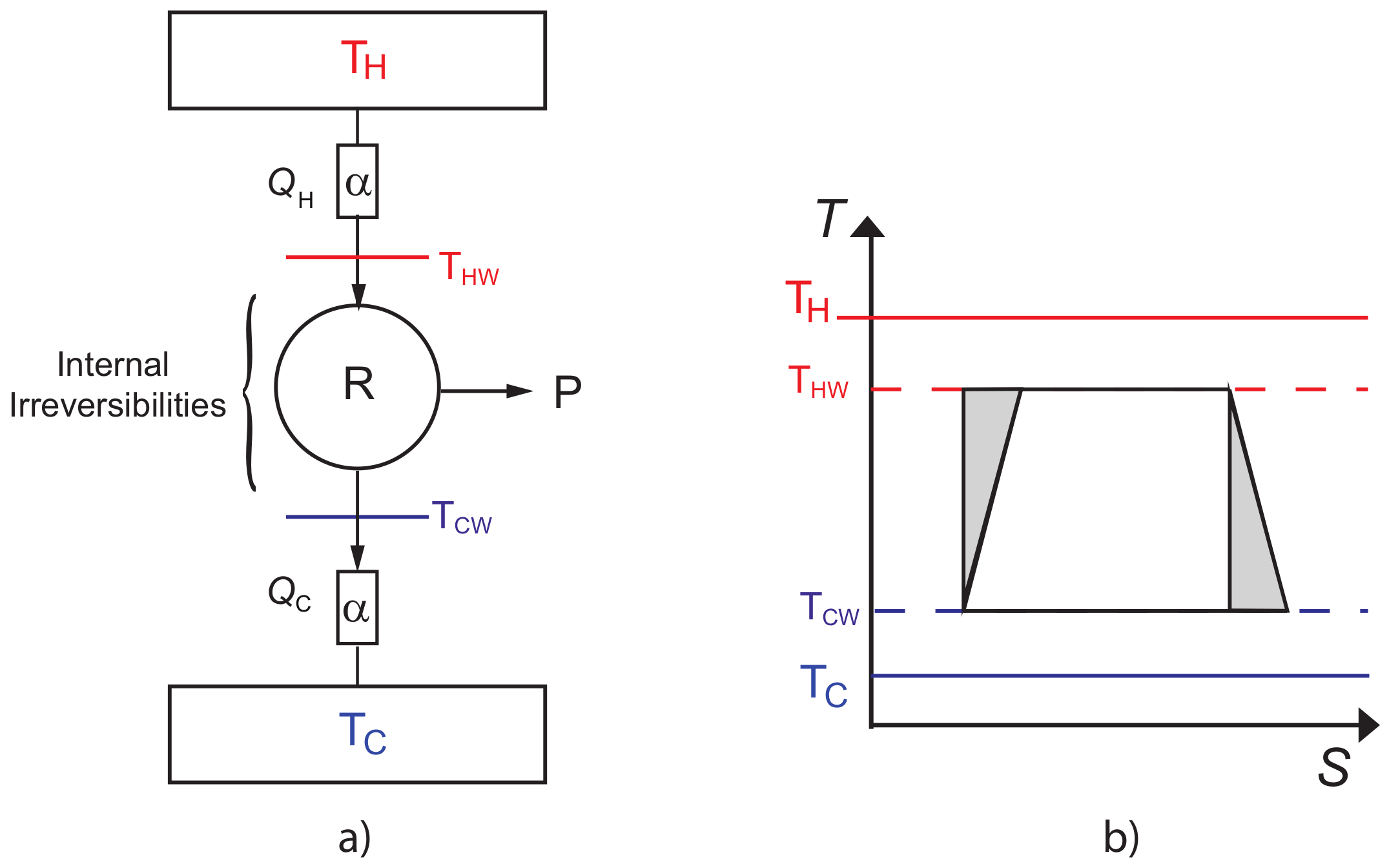
Figure 2.
(a) Plot of maximum power output vs. ; and (b) plot of efficiency at maximum power output vs. . Solid lines correspond to instant adiabatic branches (IA), and dashed lines correspond to non-instantaneous adiabatic branches (NIA). Blue lines show and green lines show .
Figure 2.
(a) Plot of maximum power output vs. ; and (b) plot of efficiency at maximum power output vs. . Solid lines correspond to instant adiabatic branches (IA), and dashed lines correspond to non-instantaneous adiabatic branches (NIA). Blue lines show and green lines show .
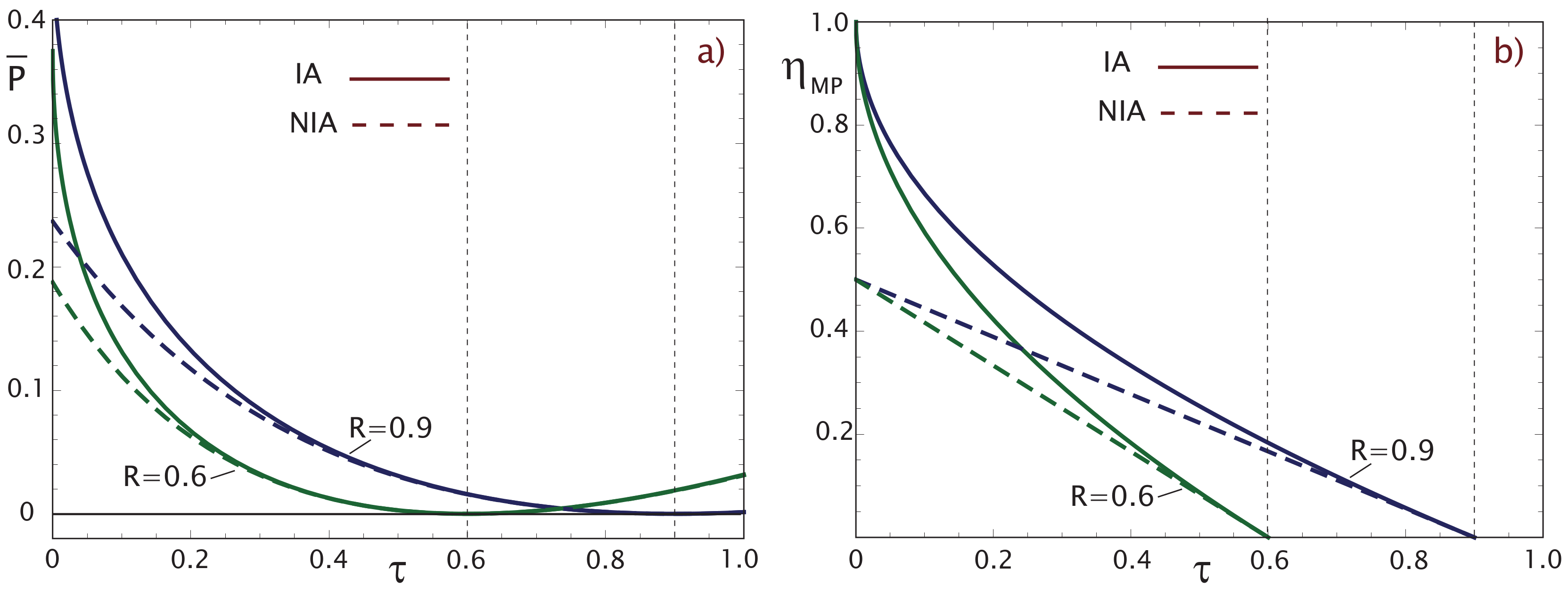
Figure 3.
(a) Plot of the power at maximum ecological function vs. ; and (b) plot of efficiency at maximum ecological function vs. . Solid lines correspond to instantaneous adiabatic branches, and dashed lines to non-instantaneous adiabatic branches. Blue lines show and green lines show .
Figure 3.
(a) Plot of the power at maximum ecological function vs. ; and (b) plot of efficiency at maximum ecological function vs. . Solid lines correspond to instantaneous adiabatic branches, and dashed lines to non-instantaneous adiabatic branches. Blue lines show and green lines show .

Figure 4.
Diagram of a Curzon–Ahlborn engine with internal irreversibilities (R), performing Carnot-like cycles between heat reservoirs and . Exchange of heat ( and ) through thermal conductors is shown, for simplicity, with the same conductance value .
Figure 4.
Diagram of a Curzon–Ahlborn engine with internal irreversibilities (R), performing Carnot-like cycles between heat reservoirs and . Exchange of heat ( and ) through thermal conductors is shown, for simplicity, with the same conductance value .
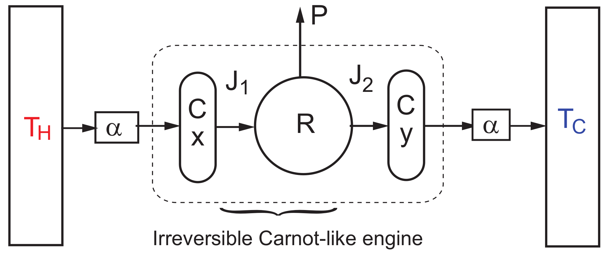
Figure 5.
Plot of relaxation times and , in units of , vs. for and , under the ecological regime with NIA branches.
Figure 5.
Plot of relaxation times and , in units of , vs. for and , under the ecological regime with NIA branches.

Figure 6.
Velocity vector field given by the ODE system in (24) and (25), with K and K. The fixed point for these parameter values is displayed with a red point.

Figure 7.
Plots of relaxation times and , in units of , vs. for . Solid lines correspond to IA and dashed lines to NIA adiabatic branches. (a) Maximum power output regime; and (b) maximum ecological function.
Figure 7.
Plots of relaxation times and , in units of , vs. for . Solid lines correspond to IA and dashed lines to NIA adiabatic branches. (a) Maximum power output regime; and (b) maximum ecological function.
© 2017 by the authors. Licensee MDPI, Basel, Switzerland. This article is an open access article distributed under the terms and conditions of the Creative Commons Attribution (CC BY) license (http://creativecommons.org/licenses/by/4.0/).
Share and Cite
MDPI and ACS Style
Paéz-Hernández, R.T.; Sánchez-Salas, N.; Chimal-Eguía, J.C.; Ladino-Luna, D. Dynamic and Thermodynamic Properties of a CA Engine with Non-Instantaneous Adiabats. Entropy 2017, 19, 632. https://doi.org/10.3390/e19110632
AMA Style
Paéz-Hernández RT, Sánchez-Salas N, Chimal-Eguía JC, Ladino-Luna D. Dynamic and Thermodynamic Properties of a CA Engine with Non-Instantaneous Adiabats. Entropy. 2017; 19(11):632. https://doi.org/10.3390/e19110632
Chicago/Turabian StylePaéz-Hernández, Ricardo T., Norma Sánchez-Salas, Juan C. Chimal-Eguía, and Delfino Ladino-Luna. 2017. "Dynamic and Thermodynamic Properties of a CA Engine with Non-Instantaneous Adiabats" Entropy 19, no. 11: 632. https://doi.org/10.3390/e19110632
Note that from the first issue of 2016, this journal uses article numbers instead of page numbers. See further details here.