On Wasserstein Two-Sample Testing and Related Families of Nonparametric Tests

Abstract

Nonparametric two-sample or homogeneity testing is a decision theoretic problem that involves identifying differences between two random variables without making parametric assumptions about their underlying distributions. The literature is old and rich, with a wide variety of statistics having being designed and analyzed, both for the unidimensional and the multivariate setting. In this short survey, we focus on test statistics that involve the Wasserstein distance. Using an entropic smoothing of the Wasserstein distance, we connect these to very different tests including multivariate methods involving energy statistics and kernel based maximum mean discrepancy and univariate methods like the Kolmogorov–Smirnov test, probability or quantile (PP/QQ) plots and receiver operating characteristic or ordinal dominance (ROC/ODC) curves. Some observations are implicit in the literature, while others seem to have not been noticed thus far. Given nonparametric two-sample testing’s classical and continued importance, we aim to provide useful connections for theorists and practitioners familiar with one subset of methods but not others.

1. Introduction

Nonparametric two-sample testing (or homogeneity testing) deals with detecting differences between two d-dimensional distributions, given samples from both, without making any parametric distributional assumptions. The popular tests for $d=1$ are rather different from those for $d>1$, and our interest is in tying together different tests used in both settings. There is massive literature on the two-sample problem, having been formally studied for nearly a century, and there is no way we can cover the breadth of this huge and historic body of work. Our aim is much more restricted—we wish to study this problem through the eyes of the versatile Wasserstein distance. We wish to form connections between several seemingly distinct families of such tests, both intuitively and formally, in the hope of informing both practitioners and theorists who may have familiarity with some sets of tests, but not others. We will also only introduce related work that has a direct relationship with this paper.

There are also a large number of tests for parametric two-sample testing (assuming a form for underlying distributions, like Gaussianity), and others for testing only differences in mean of distributions (like Hotelling’s t-test, Wilcoxon’s signed rank test, Mood’s median test). Our focus will be different from these—in this paper, we will restrict our attention only to nonparametric tests for testing differences in distributions, i.e., differences in any moment of distributions that may not have a known parametric form.

Our paper started as an attempt to understand testing with the Wasserstein distance (also called earth-mover’s distance or transportation distance). The main prior work in this area involved studying the “trimmed” comparison of distributions by [1,2] with applications to biostatistics, specifically population bioequivalence, and later by [3,4]. Apart from two-sample testing, the study of univariate goodness-of-fit testing (or one-sample testing) was undertaken in [5,6,7], and summarized exhaustively in [8]. There are other semiparametric works specific to goodness-of-fit testing for location-scale families that we do not mention here, since they diverge from our interest in fully nonparametric two-sample testing for generic distributions.

1.1. Contributions

In this survey-style paper, we uncover an interesting relationship between the multivariate Wasserstein test and the (Euclidean) Energy distance test, also called the Cramer test, proposed independently by [9,10]. This proceeds through the construction of a smoothed Wasserstein distance, by adding an entropic penalty/regularization—varying the weight of the regularization interpolates between the Wasserstein distance at one extreme and the Energy distance at the other extreme. Due to the relationship between distances and kernels, we will also establish connections to the kernel-based multivariate test by [11] called the Maximum Mean Discrepancy (MMD).

We summarize connections between the univariate Wasserstein test and popular univariate data analysis tools like quantile–quantile (QQ) plots and the Kolmogorov–Smirnov test. Finally, the desire to design a univariate distribution-free Wasserstein test will lead us to the formal study of Receiver Operating Characteristic (ROC) and Ordinal Dominance (ODC) curves, relating to work by [12].

While we connect a wide variety of popular and seemingly disparate families of tests, there are still further classes of tests that we do not have space to discuss. Some examples of tests quite different from the ones studied here include rank based tests as covered by the excellent book [13], and graphical tests that include spanning tree methods by [14] (generalizing the runs test by [15]), nearest-neighbor based tests by [16,17], and the cross-match tests by [18]. The book by [19] is also a useful reference.

1.2. Paper Outline

The rest of this paper proceeds as follows. In Section 2, we formally present the notation and setup of nonparametric two-sample testing, as well as briefly introduce three different ways of comparing distributions—using cumulative distribution functions (CDFs), quantile functions (QFs) and characteristic functions (CFs). The main contribution of this paper is Section 3, where we introduce the entropy-smoothed Wasserstein distance, and we form a novel connection between the multivariate Wasserstein distance to the multivariate Energy Distance, and to the kernel MMD. In Section 4, we discuss the relation between the univariate Wasserstein two-sample test to PP and QQ plots/tests, including the popular Kolmogorov–Smirnov test. In Section 6, we run some simulations to compare the different classes of tests discussed. Lastly, in Section 5, we will design a univariate Wasserstein test statistic that is also “distribution-free” unlike its classical counterpart, providing a careful and rigorous analysis of its limiting distribution by connecting it to ROC/ODC curves. In summary, Section 3, Section 4 and Section 5, respectively, discuss the following connections:

$$\mathrm{Wasserstein}\stackrel{\mathrm{entropic}\mathrm{smoothing}}{\to }\text{Energy Distance }(\mathrm{ED})\stackrel{\mathrm{kernels}}{\to }\mathrm{MMD};$$

$$\mathrm{Wasserstein}\stackrel{\mathrm{univariate}\mathrm{setting}}{\to }\mathrm{QQ}/\text{PP plots}\stackrel{\mathrm{change}\mathrm{of}\mathrm{norm}}{\to }\mathrm{Kolmogorov}–\mathrm{Smirnov};$$

$$\mathrm{Wasserstein}\stackrel{\mathrm{distribution}-\mathrm{free}\mathrm{variant}}{\to }\text{ODC curve}\stackrel{\mathrm{axis}\mathrm{reversal}}{\to }\text{ROC curve}.$$

We view the similarities and differences between these above tests through two lenses. The first is the population viewpoint of how different tests work with different representations of distributions; most of these tests are based on differences between quantities that completely specify a distribution—(a) CDFs; (b) QFs; and (c) CFs. The second viewpoint is the finite sample behavior of these statistics under the null hypothesis; most of these tests have null distributions based on norms of Brownian bridges, alternatively viewed as infinite sums of weighted chi-squared distributions (due to the Karhunen–Loeve expansion). We will return to these points as the paper proceeds.

2. Nonparametric Two-Sample Testing

More formally, given i.i.d. samples $X_1,...,X_n$∼P and $Y_1,...,Y_m$∼Q, where P and Q are probability measures on ${\mathbb{R}}^d$, we denote by $P_n$ and $Q_m$ the corresponding empirical measures. A test η is a function from the data $D_{n,m}:=\{X_1,...X_n,Y_1,...,Y_m\}\in {\mathbb{R}}^{d(n+m)}$ to $\{0,1\}$ (or to $[0,1]$ if it is a randomized test), where 0/1 indicates acceptance/rejection of the null hypothesis.

Most tests proceed by calculating a scalar test statistic $T_{n,m}:=T\left(D_{n,m}\right)\in \mathbb{R}$ and deciding $H_0$ or $H_1$ depending on whether $T_{n,m}$, after suitable normalization, is smaller or larger than a threshold $t_{\alpha }$. $t_{\alpha }$ is calculated based on a prespecified false positive rate α, chosen so that ${\mathbb{E}}_{H_0}\eta \le \alpha$, at least asymptotically. Indeed, all tests considered in this paper are of the form

$$\eta (X_1,...,X_n,Y_1,...,Y_m)=\mathbb{I}\left(T_{n,m}>t_{\alpha }\right).$$

We follow the Neyman–Pearson paradigm, where a test is judged by its power ${\mathbb{E}}_{H_1}\eta$ which is some function $\varphi (m,n,d,P,Q,\alpha )$. We say that a test η is consistent, in the classical sense, when

$$\varphi \to 1\mathrm{as}m,n\to \infty ,\alpha \to 0.$$

All the tests we consider in this paper will be consistent in the classical sense mentioned above. Establishing general conditions under which these tests are consistent in the high-dimensional setting is largely open. All the test statistics considered here are of the form that they are typically small under $H_0$ and large under $H_1$ (usually with appropriate scaling, they converge to zero and to infinity, respectively, with infinite samples). The aforementioned threshold $t_{\alpha }$ will be determined by the distribution of the test statistic being used under the null hypothesis (i.e., assuming the null was true, we would like to know the typical variation of the statistic, and we reject the null if our observation is far from what is typically expected under the null). This naturally leads us to study the null distribution of our test statistic, i.e., the distribution of our statistic under the null hypothesis. Since these are crucial to running and understanding the corresponding tests, we will pursue their description in detail in this paper.

2.1. Three Ways to Compare Distributions

The literature broadly has three dominant ways of comparing distributions, both in one and in multiple dimensions. These are based on three different ways of characterizing distributions—CDFs, CFs and QFs. Many of the tests we will consider involve calculating differences between (empirical estimates of) these quantities.

For example, it is well known that the Kolmogorov–Smirnov (KS) test by [20,21] involves differences in empirical CDFs. We shall later see that in one dimension, the Wasserstein distance calculates differences in QFs.

The KS test, the related Cramer von-Mises criterion by [22,23], and Anderson–Darling test by [24] are very popular in one dimension, but their usage has been more restricted in higher dimensions. This is mostly due to the curse of dimensionality involved with estimating multivariate empirical CDFs. While there has been work on generalizing these popular one-dimensional to higher dimensions, like [25], these are seemingly not the most common multivariate tests.

Kernel and distance based tests have recently gained in popularity. As we will recap in more detail in later sections, it is known that the Gaussian kernel MMD implicitly calculates a (weighted) difference in CFs and the Euclidean energy distance implicitly works with a difference in (projected) CDFs.

3. Entropy Smoothed Wasserstein Distances

The family of p-Wasserstein distances is a by-product of optimal transport theory [26]. Optimal transport can be used to compare probability measures in metric spaces; we consider here the classical case where that metric space is ${\mathbb{R}}^d$ endowed with the usual Euclidean metric.

3.1. Wasserstein Distance

Given an exponent $p\ge 1$, the definition of the p-Wasserstein distance reads:

Definition 1 (Wasserstein Distances).

For $p\in [1,\infty )$ and Borel probability measures $P,Q$ on ${\mathbb{R}}^d$ with finite p-moments, their p-Wasserstein distance ([26], Section 6) is

$$W_p(P,Q)={\left(\underset{\pi \in \Gamma (P,Q)}{inf}{\int }_{{\mathbb{R}}^d\times {\mathbb{R}}^d}{\parallel X-Y\parallel }^{p}d\pi \right)}^{1/p},$$

(1)

where $\Gamma (P,Q)$ is the set of all joint probability measures on ${\mathbb{R}}^d\times {\mathbb{R}}^d$ whose marginals are $P,Q$, i.e., for all subsets $A\subset {\mathbb{R}}^d$, we have $\pi (A\times {\mathbb{R}}^d)=P\left(A\right)$ and $\pi ({\mathbb{R}}^d\times A)=Q\left(A\right)$.

A remarkable feature of Wasserstein distances is that Definition 1 applies to all measures regardless of their absolute continuity with respect to the Lebesgue measure: The same definition works for both empirical measures and for their densities if they exist.

Writing ${\mathbf{1}}_n$ for the n-dimensional vector of ones, when comparing two empirical measures with uniform (the Wasserstein machinery works also for non-uniform weights. We do not mention this in this paper because all of the measures we consider in the context of two-sample testing are uniform) weight vectors ${\mathbf{1}}_n/n$ and ${\mathbf{1}}_m/m$, the Wasserstein distance $W_p(P_n,Q_m)$ exponentiated to the power p is the optimum of a network flow problem known as the transportation problem ([27], Section 7.2). This problem has a linear objective and a polyhedral feasible set, defined, respectively, through the matrix $M_{XY}$ of pairwise distances between elements of X and Y raised to the power p:

$$M_{XY}:=[\parallel X_i-Y_j{{\parallel }^p]}_{ij}\in {\mathbb{R}}^{n\times m},$$

(2)

and the polytope $U_{nm}$ defined as the set of $n\times m$ nonnegative matrices such that their row and column sums are equal to ${\mathbf{1}}_n/n$ and ${\mathbf{1}}_m/m$, respectively:

$$U_{nm}:=\{T\in {\mathbb{R}}_{+}^{n\times m}:T{\mathbf{1}}_m={\mathbf{1}}_n/n,T^T{\mathbf{1}}_n={\mathbf{1}}_m/m\}.$$

(3)

Let $\langle A,B\rangle :=trace\left(A^{T}B\right)$ be the usual Frobenius dot-product of matrices. Combining Equations (2) and (3), we have that $W_p^p(P_n,Q_m)$ is the optimum of a linear program S of $n\times m$ variables,

$$W_p^p(P_n,Q_m)=\underset{T\in U_{nm}}{min}\langle T,M_{XY}\rangle ,$$

(4)

of feasible set $U_{nm}$ and cost matrix $M_{XY}$.

We finish this section by pointing out that the rate of convergence as $n,m\to \infty$ of $W_p(P_n,Q_m)$ towards $W_p(P,Q)$ gets slower as the dimension d grows under mild assumptions. For simplicity of exposition, consider $m=n$. For any $p\in [1,\infty )$, it follows from [28] that for $d\ge 3$, the difference between $W_p(P_n,Q_n)$ and $W_p(P,Q)$ scales as $n^{-1/d}$. We also point out that when $d=2$, the rate actually scales as $\frac{\sqrt{ln\left(n\right)}}{\sqrt{n}}$ (see [29]). Finally, we note that when considering $p=\infty$, the rates of convergence are different to those when $1\le p<\infty$ . The work of [30,31,32] shows that the rate of convergence of $W_{\infty }(P_n,Q_n)$ towards $W_{\infty }(P,Q)$ is of the order ${\left(\frac{ln\left(n\right)}{n}\right)}^{1/d}$ when $d\ge 3$ and $\frac{{(ln\left(n\right))}^{3/4}}{n^{1/2}}$ when $d=2$. Hence, the original Wasserstein distance by itself may not be a favorable choice for a multivariate two-sample test.

3.2. Entropic Smoothing

Aside from the slow convergence rate of the Wasserstein distance between samples from two different measures to their distance in population, computing the optimum of Equation (4) is expensive. This can be easily seen by noticing that the transportation problem boils down to an optimal assignment problem when $n=m$. Since the resolution of the latter has a cubic cost in n, all known algorithms that can solve the optimal transport problem scale at least super-cubicly in n. Using an idea that can be traced back as far as Schrodinger [33], Cuturi [34] recently proposed to use an entropic regularization of the optimal transport problem, in order to define the Sinkhorn divergence between $P,Q$ parameterized by $\lambda \ge 0$ as

$$S_{\lambda }^p(P,Q):=\underset{T\in U_{nm}}{min}\lambda \langle T,M_{XY}\rangle -E\left(T\right),$$

(5)

where $E\left(T\right)$ is the entropy of T seen as a discrete joint probability distribution, namely $E\left(T\right)$: = −${\sum }_{ij}{T}_{ij}log\left(T_{ij}\right).$

This approach has two benefits: (i) because $E\left(T\right)$ is 1-strongly convex with respect to the ${\ell }_1$ norm, the regularized problem is itself strongly convex and admits a unique optimal solution, written $T_{\lambda }$, as opposed to the initial OT problem, for which the minimizer may not be unique; (ii) this optimal solution $T_{\lambda }$ is a diagonal scaling of $e^{-M_{XY}}$, the element-wise exponential matrix of $-M_{XY}$. One can easily show using the Lagrange method of multipliers that there must exist two non-negative vectors $u\in {\mathbb{R}}^n,v\in {\mathbb{R}}^m$ such that $T_{\lambda }$: =$D_u{e}^{-M_{XY}}{D}_v$, where $D_u$ $D_v$ are diagonal matrices with u and v on their diagonal. The solution to this diagonal scaling problem can be found efficiently through Sinkhorn’s algorithm [35], which has a linear convergence rate [36]. Sinkhorn’s algorithm can be implemented in a few lines of code that only require matrix vector products and elementary operations, hence they are easily parallelized on modern hardware.

3.3. Two Extremes of Smoothing: Wasserstein and Energy Distance

An interesting class of tests are distance-based “energy statistics” as introduced originally by [9], and later by [10]. The statistic, called the Cramer statistic by the latter paper and Energy Distance by the former, corresponds to the population quantity

$$\mathrm{ED}:=2\mathbb{E}\parallel X-Y\parallel -\mathbb{E}\parallel X-X^{\prime }\parallel -\mathbb{E}\parallel Y-Y^{\prime }\parallel ,$$

where $X,X^{\prime }\sim P$ and $Y,Y^{\prime }\sim Q$ (all i.i.d.). The associated test statistic is

$$\begin{array}{ccc}\hfill {\mathrm{ED}}_b& :=& \frac{2}{mn}\sum _{i=1}^n\sum _{j=1}^m\parallel X_i-Y_j\parallel -\frac{1}{n^2}\sum _{i,j=1}^n\parallel X_i-X_j\parallel -\frac{1}{m^2}\sum _{i,j=1}^m\parallel Y_i-Y_j\parallel .\hfill \end{array}$$

It was proved by the authors that $\mathrm{ED}(P,Q)=0$ iff $P=Q$. Hence, rejecting when ${\mathrm{ED}}_b$ is larger than an appropriate threshold leads to a test which is consistent against all fixed alternatives where $P\ne Q$ under mild conditions (like finiteness of $\mathbb{E}\left[X\right],\mathbb{E}\left[Y\right]$); see aforementioned references for details. Then, the Sinkhorn divergence defined in Equation (5) can be linked to the the energy distance when the parameter λ is set to $\lambda =0$— namely when only entropy is considered in the resolution of Equation (5), through the following formula:

$${\mathrm{ED}}_b=2S_0^1(P_n,Q_m)-S_0^1(P_n,P_n)-S_0^1(Q_m,Q_m).$$

(6)

Indeed, notice first that the solution to Equation (5) at $\lambda =0$ is the maximum entropy table in $U_{nm}$, namely the outer product $\left({\mathbf{1}}_n{\mathbf{1}}_m^T\right)/nm$ of the marginals ${\mathbf{1}}_n/n$ and ${\mathbf{1}}_m/m$. Hence, Equation (6) follows from the observations that

$$\begin{array}{cc}\hfill S_0^1(P_n,Q_m)& =\frac{1}{nm}\sum _{i,j}\parallel X_i-Y_j\parallel ,\hfill \\ \hfill S_0^1(P_n,P_n)& =\frac{1}{n^2}\sum _{i,j=1}^n\parallel X_i-X_j\parallel ,\hfill \\ \hfill S_0^1(Q_m,Q_m)& =\frac{1}{m^2}\sum _{i,j=1}^m\parallel Y_i-Y_j\parallel .\hfill \end{array}$$

It is also known that the population energy distance is related to the integrated difference in CDFs, i.e.,

$$\mathrm{ED}(P,Q)=\underset{(a,t)\in S^{d-1}\times \mathbb{R}}{\int }{[F_X(a,t)-F_Y(a,t)]}^2\mathrm{d}a\mathrm{d}t,$$

where $F_X(a,t)=P(a^{T}X\le t)$ (similarly $F_Y(a,t)$) is the population CDF of X when projected along direction a and $S^{d-1}$ is the surface of the d-dimensional unit sphere; see [9] for a proof.

3.4. From Energy Distance to Kernel Maximum Mean Discrepancy

Another popular class of tests that has emerged over the last decade are kernel-based tests introduced independently by [37,38], and expanded on in [11]. Without getting into technicalities that are irrelevant for this paper, the Maximum Mean Discrepancy between $P,Q$ is defined as

$$\mathrm{MMD}({\mathcal{H}}_k,P,Q):=\underset{{\parallel f\parallel }_{{\mathcal{H}}_k}\le 1}{max}{\mathbb{E}}_{P}f\left(X\right)-{\mathbb{E}}_{Q}f\left(Y\right),$$

where ${\mathcal{H}}_k$ is a Reproducing Kernel Hilbert Space associated with Mercer kernel $k(·,·)$, and ${\parallel f\parallel }_{{\mathcal{H}}_k}\le 1$ is its unit norm ball.

While it is easy to see that $\mathrm{MMD}\ge 0$ always, and also that $P=Q$ implies $\mathrm{MMD}=0$, Reference [37] shows that if k is “characteristic”, the equality holds iff $P=Q$. The Gaussian kernel $k(a,b)=exp(-\parallel a-b{\parallel }^2/{\gamma }^2)$ is a popular example of a characteristic kernel, and in this case, $\mathrm{MMD}$ can be interpreted as the integrated difference between characteristic functions. Indeed, by Bochner’s theorem (see [39]), the population quantity ${\mathrm{MMD}}^2$ with the Gaussian kernel is precisely (up to constants)

$${\int }_{{\mathbb{R}}^d}{|{\phi }_X\left(t\right)-{\phi }_Y\left(t\right)|}^2{e}^{-{\gamma }^2{\parallel t\parallel }^2}\mathrm{d}t,$$

where ${\phi }_X\left(t\right)={\mathbb{E}}_{x\sim P}\left[e^{-i{t}^{T}x}\right]$ is the characteristic function of X at frequency t (similarly ${\phi }_Y\left(t\right)$). Using the Riesz representation theorem and the reproducing property of ${\mathcal{H}}_k$, one can argue that $\mathrm{MMD}({\mathcal{H}}_k,P,Q)={\parallel {\mathbb{E}}_{P}k(X,.)-{\mathbb{E}}_{Q}k(Y,.)\parallel }_{{\mathcal{H}}_k}$ and conclude that

$${\mathrm{MMD}}^2=\mathbb{E}k(X,X^{\prime })+\mathbb{E}k(Y,Y^{\prime })-2\mathbb{E}k(X,Y).$$

This gives rise to a natural associated test statistic, a plugin estimator of ${\mathrm{MMD}}^2$:

$$\begin{array}{ccc}\hfill {\mathrm{MMD}}_u^2\left(k(·,·)\right)& :=& \frac{1}{n^2}\sum _{i,j=1}^{n}k(X_i,X_j)+\frac{1}{m^2}\sum _{i,j=1}^{m}k(Y_i,Y_j)-\frac{2}{mn}\sum _{i=1}^n\sum _{j=1}^{m}k(X_i,Y_j).\hfill \end{array}$$

At first sight, the Energy Distance and the MMD look like fairly different tests. However, there is a natural connection that proceeds in two steps. Firstly, there is no reason to stick to only the Euclidean norm ${\parallel ·\parallel }_2$ to measure distances for ED—the test can be extended to other norms, and in fact also other metrics; Reference [40] explains the details for the closely related independence testing problem. Following that, Reference [41] discusses the relationship between distances and kernels (again for independence testing, but the same arguments also hold in the two-sample testing setting). Loosely speaking, for every kernel k, there exists a metric d (and also vice versa), given by $d(x,y):=\left(k\right(x,x)+k(y,y\left)\right)/2-k(x,y)$, such that MMD with kernel k equals ED with metric d. This is a very strong connection between these two families of tests—the energy distance is a special case of the kernel MMD, corresponding to a particular choice of kernel, and the kernel MMD itself corresponds to an extremely smoothed Wasserstein distance, for a particular choice of distance.

4. Univariate Wasserstein Distance and PP/QQ Tests

For univariate random variables, a PP plot is a graphical way to view differences in empirical CDFs, while QQ plots are analogous to comparing QFs. Instead of relying on graphs, we can also make such tests more formal and rigorous as follows. We first present some results on the asymptotic distribution of the difference between $P_n$ and $Q_m$ when using the distance between the CDFs $F_n$ and $G_m$ and then later when using the distance between the QFs $F_n^{-1}$ and $G_m^{-1}$. For simplicity, we assume that both distributions P and Q are supported on the interval $[0,1]$; we remark that under mild assumptions on P and Q, the results we present in this section still hold without such a boundedness assumption. We assume for simplicity that the CDFs F and G have positive densities on $[0,1]$.

4.1. Comparing CDFs (PP)

We start by noting $F_n$ may be interpreted as a random element taking values in the space $\mathcal{D}\left(\right[0,1\left]\right)$ of right continuous functions with left limits. It is well known that

$$\sqrt{n}\left(F_n-F\right){\to }_w\mathbb{B}\circ F,$$

(7)

where $\mathbb{B}$ is a standard Brownian bridge in $[0,1]$ and where the weak convergence ${\to }_w$ is understood as convergence of probability measures in the space $\mathcal{D}\left(\right[0,1\left]\right)$; see Chapter 3 in [42] for details. From this fact and the independence of the samples, it follows that under the null hypothesis $H_0:P=Q$, as $n,m\to \infty$

$$\sqrt{\frac{mn}{n+m}}\left(F_n-G_m\right)=\sqrt{\frac{mn}{n+m}}\left(F_n-F\right)+\sqrt{\frac{mn}{n+m}}\left(G-G_m\right){\to }_w\mathbb{B}\circ F.$$

(8)

The previous fact and continuity of the function $h\in \mathcal{D}\left([0,1]\right)\mapsto {\int }_0^1{\left(h\left(t\right)\right)}^{2}dt$ imply that as $n,m\to \infty$, we have under the null,

$$\frac{mn}{n+m}{\int }_0^1{\left(F_n\left(t\right)-G_m\left(t\right)\right)}^{2}dt{\to }_w{\int }_0^1{\left(\mathbb{B}\left(F\left(t\right)\right)\right)}^{2}dt.$$

(9)

Observe that the above asymptotic null distribution depends on F, which is unknown in practice. This is an obstacle when considering any $L^p$-distance, with $1\le p<\infty$, between the empirical cdfs $F_n$ and $G_m$. Luckily, a different situation occurs when one considers the $L^{\infty }$-distance between $F_n$ and $G_m$. Under the null, using Equation (7) again, we deduce that

$$\sqrt{\frac{mn}{n+m}}\parallel F_n-G_m{\parallel }_{\infty }{\to }_w{\parallel \mathbb{B}\circ F\parallel }_{\infty }={\parallel \mathbb{B}\parallel }_{\infty },$$

(10)

where the equality in the previous expression follows from the fact that the continuity of F implies that the interval $[0,1]$ is mapped onto the interval $[0,1]$. This is known as the Kolmogorov–Smirnov test, and is hence appropriate for two-sample problems. A related statistic, called the Anderson-Darling test, will also be considered in the experiments.

4.2. Comparing QFs (QQ)

We now turn our attention to QQ (quantile–quantile) plots and specifically the $L^2$-distance between $F_n^{-1}$ and $G_m^{-1}$. It can be shown that if F has a differentiable density f which (for the sake of simplicity) we assume is bounded away from zero, then

$$\sqrt{n}(F_n^{-1}-F^{-1}){\to }_w\frac{\mathbb{B}}{f\circ F^{-1}}.$$

For a proof of the above statement, see Chapter 18 in [43]; for an alternative proof where the weak convergence is considered in the space of probability measures on $L^2\left((0,1)\right)$ (as opposed to the space $\mathcal{D}\left(\right[0,1\left]\right)$ we have been considering thus far), see [8]. We note that from the previous result and independence, it follows that under the null hypothesis $H_0:P=Q$,

$$\sqrt{\frac{mn}{n+m}}(F_n^{-1}-G_m^{-1}){\to }_w\frac{\mathbb{B}}{f\circ F^{-1}}.$$

In particular, by continuity of the function $h\in L^2\left((0,1)\right)\mapsto {\int }_0^1{\left(h\left(t\right)\right)}^{2}dt$, we deduce that

$$\frac{mn}{n+m}{\int }_0^1{(F_n^{-1}-G_m^{-1})}^{2}dt{\to }_w{\int }_0^1\frac{{\left(\mathbb{B}\left(t\right)\right)}^2}{{(f\circ F^{-1}\left(t\right))}^2}dt.$$

Hence, as was the case when we considered the difference of the cdfs $F_n$ and $G_m$, the asymptotic distribution of the $L^2$-difference (or analogously any $L^p$-difference for finite p) of the empirical quantile functions is also distribution dependent. Note, however, that there is an important difference between QQ and PP plots when using the $L^{\infty }$ norm. We saw that the asymptotic distribution of the $L^{\infty }$ norm of the difference of $F_n$ and $G_m$ is (under the null hypothesis) distribution free. Unfortunately, in the quantile case, we obtain

$$\sqrt{\frac{mn}{n+m}}\parallel F_n^{-1}-G_n^{-1}{\parallel }_{\infty }{\to }_w{\parallel \frac{\mathbb{B}}{f\circ F^{-1}}\parallel }_{\infty },$$

which, of course, is distribution dependent. Since one would have to resort to computer-intensive Monte-Carlo techniques (like bootstrap or permutation testing) to control type-1 error, these tests are sometimes overlooked (though with modern computing speeds, they merit further study).

4.3. Wasserstein Is a QQ Test

Recall that, for $p\in [1,\infty )$, the p-Wasserstein distance between two probability measures $P,Q$ on $\mathbb{R}$ with finite p-moments is given by Equation (1).

Because the Wasserstein distance measures the cost of transporting mass from the original distribution P into the target distribution Q, one can say that it measures “horizontal” discrepancies between P and Q. Intuitively, two probability distributions P and Q that are different over “long” (horizontal) regions will be far away from each other in the Wasserstein distance sense because, in that case, mass has to travel long distances to go from the original distribution to the target distribution. In the one-dimensional case (in contrast with what happens in dimension $d>1$), the p-Wasserstein distance has a simple interpretation in terms of the quantile functions $F^{-1}$ and $G^{-1}$ of P and Q, respectively. The reason for this is that the optimal way to transport mass from P to Q has to satisfy a certain monotonicity property that we describe in the proof of the following proposition. This is a well known fact that can be found, for example, in [19].

Proposition 1.

The p-Wasserstein distance between two probability measures P and Q on $\mathbb{R}$ with p-finite moments can be written as

$$W_p^p(P,Q)={\int }_0^1{|F^{-1}\left(t\right)-G^{-1}\left(t\right)|}^{p}dt,$$

where $F^{-1}$ and $G^{-1}$ are the quantile functions of P and Q, respectively.

Having considered the p-Wasserstein distance $W_p(P,Q)$ for $p\in [1,\infty )$ in Proposition 1, we conclude this section by considering the case $p=\infty$. Let $P,Q$ be two probability measures on $\mathbb{R}$ with bounded support. That is, assume that there exists a number $N>0$ such that $supp\left(P\right)\subseteq [-N,N]$ and $supp\left(Q\right)\subseteq [-N,N]$. We define the ∞-Wasserstein distance between P and Q by

$$W_{\infty }(P,Q):=\underset{\pi \in \Gamma (P,Q)}{inf}esssu{p}_{\pi }|x-y|.$$

Proceeding as in the case $p\in [1,\infty )$, it is possible to show that the ∞-Wasserstein distance between P and Q with bounded supports can be written in terms of the difference of the corresponding quantile functions as

$$W_{\infty }(P,Q)={\parallel F^{-1}-G^{-1}\parallel }_{\infty }.$$

The Wasserstein distance is called the Mallow’s distance in the statistical literature, where it has been studied due to its ability to capture weak convergence precisely—$W_p(F_n,F)$ converges to 0 if and only if $F_n$ converges in distribution to F and also the p-th moment of X under $F_n$ converges to the corresponding moment under F; see [44,45,46]. It is also related to the Kantorovich–Rubinstein metric from optimal transport theory.

5. Distribution-Free Wasserstein Tests and ROC/ODC Curves

As we earlier saw, under $H_0:P=Q$, the statistic $\frac{mn}{n+m}{\int }_0^1{\left(F_n^{-1}\left(t\right)-G_m^{-1}\left(t\right)\right)}^{2}dt$ has an asymptotic distribution that is not distribution free, i.e., it depends on F. We also saw that as opposed to what happens with the asymptotic distribution of the $L^{\infty }$ distance between $F_n$ and $G_m$, the asymptotic distribution of $\parallel F_n^{-1}-G_m^{-1}{\parallel }_{\infty }$ does depend on the cdf F. In this section, we show how we can construct a distribution-free Wasserstein test by connecting it to the theory of ROC and ODC curves.

5.1. Relating Wasserstein Distance to ROC and ODC Curves

Let P and Q be two distributions on $\mathbb{R}$ with cdfs F and G and quantile functions $F^{-1}$ and $G^{-1}$, respectively. We define the ROC curve between F and G as the function.

$$ROC\left(t\right):=1-F\left(G^{-1}(1-t)\right),t\in [0,1].$$

In addition, we define their ODC curve by

$$ODC\left(t\right):=G\left(F^{-1}\left(t\right)\right),t\in [0,1].$$

The following are properties of the ROC curve (see [12]):

• The $ROC$ curve is increasing and $ROC\left(0\right)=0$, $ROC\left(1\right)=1$.
• If $G\left(t\right)\ge F\left(t\right)$ for all t, then $ROC\left(t\right)\ge t$ for all t.
• If $F,G$ have densities with monotone likelihood ratio, then the ROC curve is concave.
• The area under the ROC curve is equal to $\mathbb{P}(Y<X)$, where Y∼Q and X∼P.

Intuitively speaking, the faster the ROC curve increases towards the value 1, the easier it is to distinguish the distributions P and Q. Observe from their definitions that the ROC curve can be obtained from the ODC curve after reversing the axes. Given this, we focus from this point on only one of them, the ODC curve being more convenient.

The first observation about the ODC curve is that it can be regarded as the quantile function of the distribution $G_{♯}P$ (the push forward of P by G) on $[0,1]$, which is defined by

$$G_{♯}P\left([0,\alpha )\right):=P\left(G^{-1}\left([0,\alpha )\right)\right),\alpha \in [0,1].$$

Similarly, we can consider the measure ${G_m}_{♯}{P}_n$, that is, the push forward of $P_n$ by $G_m$. We crucially note that the empirical ODC curve $G_m\circ F_n^{-1}$ is the quantile function of ${G_m}_{♯}{P}_n$. From Section 4, we deduce that

$$W_p^p({G_m}_{♯}{P}_n,G_{♯}P)={\int }_0^1{|G_m\circ F_n^{-1}\left(t\right)-G\circ F^{-1}\left(t\right)|}^{p}dt$$

for every $p\in [1,\infty )$ and also

$$W_{\infty }({G_m}_{♯}{P}_n,G_{♯}P)={\left||G_m\circ F_n^{-1}-G\circ F^{-1}|\right|}_{\infty }.$$

That is, the p-Wasserstein distance between the measures ${G_m}_{♯}{P}_n$ and $G_{♯}P$ can be computed by considering the $L^p$ distance of the ODC curve and its empirical version.

First, we argue that under the null hypothesis $H_0:P=Q$, the distribution of the empirical ODC curve is actually independent of P. In particular, $W_p^p({G_m}_{♯}{P}_n,G_{♯}P)$ and $W_{\infty }({G_m}_{♯}{P}_n,G_{♯}P)$ are distribution free under the null! This is the content of the next lemma, proved in the Appendix.

Lemma 1 (Reduction to uniform distribution).

Let $F,G$ be two continuous and strictly increasing CDFs and let $F_n$ and $G_m$ be the empirical CDFs. Consider the (unknown) random variables, which are distributed uniformly on $[0,1]$,

$$U_k^X:=F\left(X_k\right),U_k^Y:=G\left(Y_k\right).$$

Let $F_n^U$ be the empirical CDF associated with the (uniform) $U^X$s and let $G_m^U$ be the empirical CDF associated with the (uniform) $U^Y$s. Then, under the null $H_0:F=G$, we have

$$G_m\left(X_k\right)=G_m^U\left(U_k^X\right),\forall k\in \left\{1,\cdots ,n\right\}.$$

In particular, we have $G_m\circ F_n^{-1}\left(t\right)=G_m^U\circ {F_n^U}^{-1}\left(t\right),\forall t\in [0,1].$

Proof. 

We denote by $Y_{\left(1\right)}\le \cdots \le Y_{\left(m\right)}$ the order statistic associated to the Ys. For $k=1,\cdots ,m-1$ and $t\in (0,1)$, we have $G_m\left(t\right)=\frac{k}{m}$ if and only if $t\in [Y_{\left(k\right)},Y_{(k+1)})$, which holds if and only if $t\in [F^{-1}\left(U_{\left(k\right)}^Y\right),F^{-1}\left(U_{(k+1)}^Y\right))$, which, in turn, is equivalent to $F\left(t\right)\in [U_{\left(k\right)}^Y,U_{(k+1)}^Y)$. Thus, $G_m\left(t\right)=\frac{k}{m}$ if and only if $G_m^U\left(F\left(t\right)\right)=\frac{k}{m}$. From the previous observations, we conclude that $G_m=G_m^U\circ F$. Finally, since $X_k=F^{-1}\left(U_k^X\right)$, we conclude that

$$G_m\left(X_k\right)=G_m^U\circ F\circ F^{-1}\left(U_k^X\right)=G_m^U\left(U_k^X\right).$$

This concludes the proof. ☐

Note that since $U_k^X,U_k^Y$ are obviously instantiations of uniformly distributed random variables, the right hand side of the last equation only involves uniform random variables, and hence the distribution of $G_m\circ F_n^{-1}$ is independent of $F,G$ under the null. Now, we are almost done, and this above lemma will imply that the Wasserstein distance between $G_m\circ F_n^{-1}$ and the uniform distribution $U[0,1]$ (since $G\circ F^{-1}\left(t\right)=t=U^{-1}\left(t\right)=U\left(t\right)$ for $t\in [0,1]$ when $G=F$) also does not depend on $F,G$.

More formally, one may establish a result on the asymptotic distribution of the statistic $W_p^p({G_m}_{♯}{P}_n,G_{♯}P)$ and $W_{\infty }({G_m}_{♯}{P}_n,G_{♯}P)$. We do this by first considering the asymptotic distribution of the difference between the empirical ODC curve and the population ODC curve regarding both of them as elements in the space $\mathcal{D}\left(\right[0,1\left]\right)$. This is the content of the following Theorem which follows directly from the work of [47] (see [12]).

Theorem 1.

Suppose that F and G are two CDFs with densities $f,g$ satisfying

$$\frac{g\left(F^{-1}\left(t\right)\right)}{f\left(F^{-1}\left(t\right)\right)}\le C,$$

for all $t\in [0,1]$. In addition, assume that $\frac{n}{m}\to \lambda \in [0,\infty )$ as $n,m\to \infty$. Then,

$$\sqrt{\frac{mn}{n+m}}\left(G_m\left(F_n^{-1}(·)\right)-G\left(F^{-1}(·)\right)\right){\to }_w\sqrt{\frac{\lambda }{\lambda +1}}{B}_1(G\circ F^{-1}(·))+\sqrt{\frac{1}{\lambda +1}}\frac{g\left(F^{-1}(·)\right)}{f\left(F^{-1}(·)\right)}{B}_2(·),$$

where $B_1$ and $B_2$ are two independent Brownian bridges and where the weak convergence must be interpreted as weak convergence in the space of probability measures on the space $\mathcal{D}\left(\right[0,1\left]\right)$.

As a corollary, under the null hypothesis $H_0$: $P=Q$, we obtain the following. Suppose that the CDF F of P is continuous and strictly increasing. Then,

$$\begin{array}{cc}\hfill \frac{mn}{n+m}{W}_2^2({G_m}_{♯}{P}_n,G_{♯}P)& =\frac{mn}{n+m}{\int }_0^1{(G_m\left(F_n^{-1}\left(t\right)\right)-t)}^{2}dt{\to }_w{\int }_0^1{\left(\mathbb{B}\left(t\right)\right)}^{2}dt,\hfill \end{array}$$

(11)

$$\begin{array}{cc}\hfill \sqrt{\frac{mn}{n+m}}{W}_{\infty }({G_m}_{♯}{P}_n,G_{♯}P)& =\sqrt{\frac{mn}{n+m}}\underset{t\in [0,1]}{sup}|G_m\left(F_n^{-1}\left(t\right)\right)-t|{\to }_w\underset{t\in [0,1]}{sup}\left|\mathbb{B}\left(t\right)\right|.\hfill \end{array}$$

(12)

To see this, note that by Lemma 1 that it suffices to consider $F\left(t\right)=t$ in $[0,1]$. In that case, the assumptions of Theorem 1 are satisfied and the result follows directly. The latter test based on the infinity norm is extremely similar to the Kolmogorov–Smirnov test in theory and practice—one may also note the similarity of the above expressions with Equations (9) and (10).

The takeaway message of this section is that instead of considering the Wasserstein distance between $F_m$ and $G_n$, whose null distribution depends on unknown F, one can instead consider the Wasserstein distance between $G_m\left(F_n^{-1}\right)$ and the uniform distribution $U[0,1]$, since its null distribution is independent of F.

6. Experiments

One cannot, in general, have results comparing the powers of different nonparametric tests. Which test achieves a higher power depends on the class of alternatives being considered—some tests are more sensitive to deviations near the median, others are more sensitive to differences in the tails, and yet others are more sensitive to deviations that are not represented in the original space but instead in an underlying Hilbert space embedding of distributions (MMD and ED are examples of this). Hence, the statistical literature has very sparse results on theoretical comparisons between distributions, and one must often resort to experiments to get a sense of their relative performance on examples of interest.

In this section, we report results for two-sample tests run with the following example distributions (the parameters for the k-th pair of distributions (for $k=1,2,3,4$) so that the distributions have their first k-1 central moments as identical, but differ in their k-th central moments):

• Beta(2,2) versus Beta(1.8,2.16);
• Exponential(1), equivalently Gamma(1,1), versus Gamma(2,0.5);
• Standard Normal versus Student’s t;
• Generalized extreme value versus Generalized Pareto.

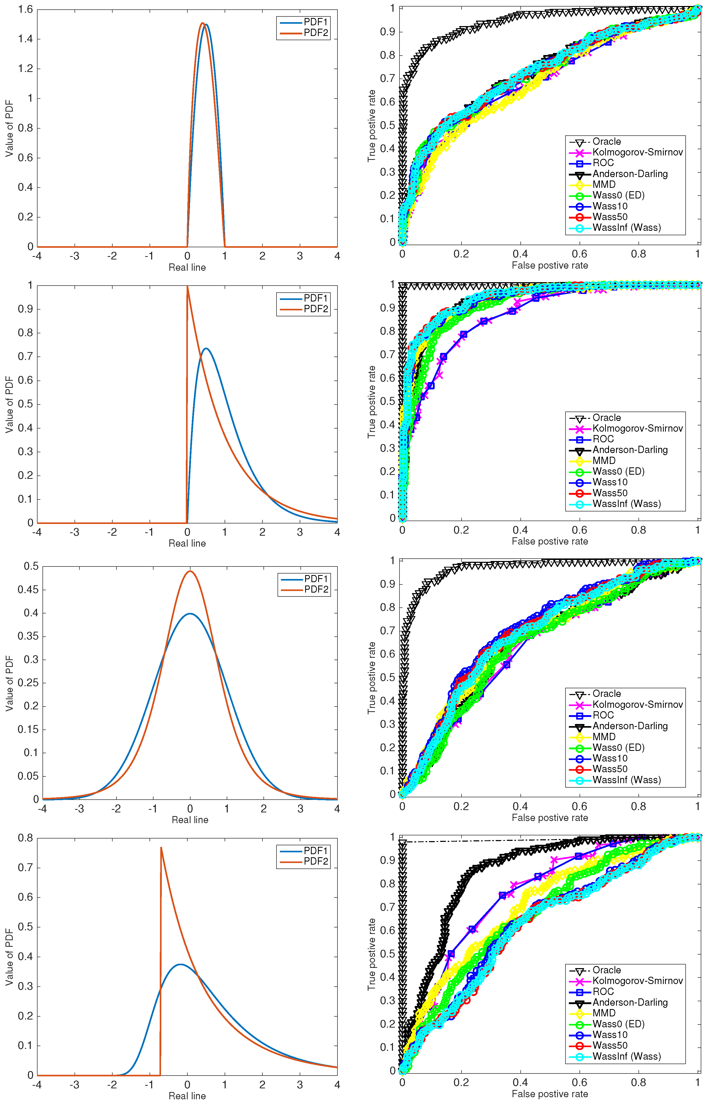
We use some common test statistics that have already been mentioned in this paper—Kolmogorov–Smirnov, Anderson–Darling, Maximum Mean Discrepancy (MMD), ROC (infinity norm) and the smoothed Wasserstein distance with four regularizations: 0 (corresponding to Energy Distance), 10, 50 and infinity (corresponding to Wasserstein distance).

All of these statistics are nonparametric, in the sense that they do not assume a particular form or have access to the true underlying PDFs. Nevertheless, all of the examples that we construct are parametric, so we also include the “oracle” likelihood ratio test (we term it as an oracle since it uses extra knowledge, namely the exact form of the PDFs, to which the other tests do not have access).

One may note from Figure 1 that the precision-recall curve of nonparametric tests are often much worse than the oracle likelihood ratio test, and this is indeed to be expected—the true utility of the nonparametric tests would be observed in a real-world example where one wishes to abstain from making any (possibly wrong, biased or misleading) parametric assumptions. As might be expected from the discussion at the start of the section, the tests are rather difficult to compare. Among the tests considered, the ordering of the curves changes over different experiments, and even within the class of Wasserstein tests. While general comparisons are difficult, there is a need for theoretical analysis comparing classes of tests in special cases of practical interest (for example, mean-separated Gaussians).

The role of entropic smoothing parameter λ is also currently unclear, and whether there is a data dependent way to pick it so as to maximize power. This could be an interesting direction of future research.

7. Conclusions

In this paper, we connect a wide variety of univariate and multivariate test statistics, with the central piece being the Wasserstein distance. The Wasserstein statistic is closely related to univariate tests like the Kolmogorov–Smirnov test, graphical QQ plots, and a distribution-free variant of the test is proposed by connecting it to ROC/ODC curves. Through entropic smoothing, the Wasserstein test is also related to the multivariate tests of Energy Distance and hence transitively to the Kernel Maximum Mean Discrepancy. We hope that this is a useful resource to connect the different families of two-sample tests, many of which can be analyzed under the two umbrellas of our paper—whether they differentiate between CDFs, QFs or CFs, and what their null distributions look like. Many questions remain open—for example, the role of smoothing parameter λ.