Response Surface Methodology Control Rod Position Optimization of a Pressurized Water Reactor Core Considering Both High Safety and Low Energy Dissipation

Abstract

Response Surface Methodology (RSM) is introduced to optimize the control rod positions in a pressurized water reactor (PWR) core. The widely used 3D-IAEA benchmark problem is selected as the typical PWR core and the neutron flux field is solved. Besides, some additional thermal parameters are assumed to obtain the temperature distribution. Then the total and local entropy production is calculated to evaluate the energy dissipation. Using RSM, three directions of optimization are taken, which aim to determine the minimum of power peak factor P_max, peak temperature T_max and total entropy production S_tot. These parameters reflect the safety and energy dissipation in the core. Finally, an optimization scheme was obtained, which reduced P_max, T_max and S_tot by 23%, 8.7% and 16%, respectively. The optimization results are satisfactory.

1. Introduction

In China, energy consumption has grown rapidly driven by the improvement of the economic level. In order to balance economic development and environmental protection, China’s government has established a green development strategy. An important measure is to adjust the energy structure and promote the consumption of clean energy sources such as nuclear energy. Thus, the use of nuclear energy increased from 44.19 billion kWh in 2000 to 290.75 billion kWh in 2013 [1], and 26 nuclear power units (28,528 MWe) are currently under construction in China [2,3].

The design of a nuclear reactor system includes shielding design, thermodynamics, fluid flow and heat transfer, fuel element design, radioactivity releases, etc. [4]. In nuclear physics calculations, the neutron flux density and its distribution are usually the primary target. The Neutron Transport Equation (NTE) is used to describe the variation of neutron flux density in a physical field. For simplification, the Neutron Diffusion Equation (NDE) is also used. These equations can be solved by the Finite Different Method (FDM) [5,6,7], the Finite Volume Method (FVM) [8,9,10,11], the Finite Element Method (FEM) [10,12,13,14], etc. Normally, the neutron flux density distribution matches the fission heat source distribution.

Heat transfer is also an important physical process in nuclear reactor core. It is an irreversible process which increases the entropy of the whole system. The differences in heat transfer in different regions causes a distribution of local entropy production. In 1979, Bejan [15] presented the fundamental equations describing entropy production due to finite temperature gradients and fluid flow. Then Bejan [16,17,18] discussed the irreversibility in thermodynamic systems by entropy production analysis. Since then, many researchers have started to use the entropy production method to evaluate heat transfer processes in various structures. For example, Ibáñez et al. [19] investigated the entropy production minimization of a solid slab with uniform internal heating and asymmetric convective cooling. Makinde and Aziz [20] analyzed the inherent irreversibility and thermal stability in the model of a long hollow cylinder with temperature-dependent internal heating and asymmetric convective cooling boundaries. Aziz and Khan [21] analyzed the entropy production of steady conduction in the model of a hollow sphere with temperature-dependent internal heating and asymmetric convective cooling boundaries. Malvandi et al. [22] studied the entropy production of steady two-dimensional boundary layer flow of nano-fluids over a flat plate. Torabi and Zhang [23] used classical entropy production analysis to investigate heat transfer in cooled homogenous and functionally graded material slabs with variation of internal heat generation with temperature, and convective-radiative boundaries.

For coupling the neutronic and thermal-hydraulic calculation, the traditional technique is the Operator Splitting (OS) method [24,25]. By this method, different physical processes are solved separately. The output of neutronic calculation is the input of thermal-hydraulic part. Some other advanced multi-physics algorithms have also been developed. One of the most famous algorithms is the Jacobian-Free Newton-Krylov (JFNK) method [26,27]. By the JFNK method, several physical processes are treated together as an entire unit. The biggest advantage of the OS method is its ease of implementation, while JFNK is more suitable for nonlinear problems and has higher accuracy.

Response Surface Methodology (RSM) is a collection of mathematical and statistical techniques used to explore the relationships between several independent variables and one or more response variables. This methodology was proposed by Box and Wilson in the 1950s [28,29]. Since then this methodology has been widely used in analytical chemistry [28], bioprocessing [29,30], structural reliability [31,32], food chemistry [33,34,35], etc. The biggest advantage of this methodology is that the RSM model is easy and convenient to establish, even when little information about the process can be obtained.

This paper aimed to optimize the insertion positions of the control rods in a Pressurized Water Reactor (PWR). The neutron diffusion and heat transfer processes are coupled and both high safety and low energy dissipation are taken into consideration. The chosen safety factors are the power peak factor and maximum temperature in the core, and the energy dissipation is calculated by the entropy production method. RSM is utilized to find a more improved scheme.

2. Description of Problem

The International Atomic Energy Agency (IAEA) has published a three-dimensional PWR benchmark problem named the 3D-IAEA [36]. It is a typical PWR problem which is widely used in verification of neutron diffusion calculation codes. This PWR is taken as a study object in this paper to demonstrate the RSM optimization of control rod insertion positions. The nuclear data given in [36] are used to solve the neutron flux distribution. Some essential thermal parameters are also assumed to calculate the temperature field and local and total entropy production.

There are 177 groups of Fuel Assemblies (FAs) arranged in the reactor core, and 13 groups of these FAs are have inserted control rods. Five kinds of materials are applied in this core. A quarter of horizontal and one half of vertical cross section of the 3D-IAEA problem are illustrated in Figure 1 and Figure 2, respectively. The multi-group neutron diffusion approximation that most widely used for commercial reactors is the two-energy groups approximation [37,38], which is also applied in 3D-IAEA benchmark problem. The neutron energy spectrum is divided into two groups, which are called fast and thermal neutrons, respectively. The two-group nuclear data are given in

Table 1. Two-group nuclear data.

Region	D1	D2	Σs,1→2	Σa1	Σa2	υΣf	Material
1	1.5	0.4	0.02	0.01	0.08	0.135	Fuel 1
2	1.5	0.4	0.02	0.01	0.085	0.135	Fuel 1
3	1.5	0.4	0.02	0.01	0.13	0.135	Fuel 2 + Rod
4	2.0	0.3	0.04	0	0.01	0	Reflector
5	2.0	0.3	0.04	0	0.055	0	Refl. + Rod

. Some additional thermal parameters are given in

Table 2. Additional thermal parameters.

Parameter	Pcore/MW	λ/W·m−1·K−1					Tboundary/K
		λ1	λ2	λ3	λ4	λ5
Value	10	5	5.25	5.25	5	5	400

.

3. Numerical Methodology

3.1. Neutron Diffusion

The NTE based on transport theory can describe the neutron behaviors in more details, but to balance of amount of calculation and perduring accuracy, in the engineering area the diffusion theory and NDE are always used to solve the neutron flux, which can be written as:

$$\begin{array}{l}\left[\frac{1}{v_g}\frac{\partial }{\partial t}-\nabla ·D_g(\overrightarrow{r},t)\nabla +{\mathrm{\Sigma }}_{t,g}(\overrightarrow{r},t)\right]{\phi }_g(\overrightarrow{r},t)\\ ={\displaystyle \sum _{g^{\prime }=1}^G{\sum }_{s,g^{\prime }\to g}(\overrightarrow{r},t){\phi }_{g^{\prime }}(\overrightarrow{r},t)}+\frac{1}{k_{\mathrm{eff}}}{\chi }_g{\displaystyle \sum _{g^{\prime }=1}^G{\upsilon }_{g^{\prime }}{\mathrm{\Sigma }}_{f,g^{\prime }}(\overrightarrow{r},t){\phi }_{g^{\prime }}(\overrightarrow{r},t)}+S_{e,g}(\overrightarrow{r},t)\end{array}$$

(1)

where g is the index of energy group, g = 1,2,…,G; G is the total number which the energy spectrum is divided into; v is the velocity of neutrons, cm·s⁻¹; t is the time, s; D is the diffusion constant, cm; Σ_t is the total cross section, cm⁻¹; Σ_s,g’→g is the scattering cross section from g’ energy group to g energy group, cm⁻¹; Σ_f is the fission cross section, cm⁻¹; $\overrightarrow{r}$ is the position, cm; φ is the neutron scalar flux density, neutrons·cm⁻²·s⁻¹; υ is the average number of neutrons that are emitted from each fission process; χ is the fission spectrum function; k_eff is the multiplication factor; S_e is the extra neutron source, neutrons·cm⁻³·s⁻¹.

When using in time independent problem with no extra neutron source and no upscattering neutrons, Equation (1) can be simplified as:

$$-\nabla D_g(\overrightarrow{r})\nabla {\phi }_g(\overrightarrow{r})+{\mathrm{\Sigma }}_{t,g}(\overrightarrow{r}){\phi }_g(\overrightarrow{r})={\displaystyle \sum _{g^{\prime }=1}^{g-1}{\sum }_{s,g^{\prime }\to g}(\overrightarrow{r}){\phi }_{g^{\prime }}(\overrightarrow{r})}+\frac{1}{k_{\mathrm{eff}}}{\chi }_g{\displaystyle \sum _{g^{\prime }=1}^G{\upsilon }_{g^{\prime }}{\mathrm{\Sigma }}_{f,g^{\prime }}(\overrightarrow{r}){\phi }_{g^{\prime }}(\overrightarrow{r})}$$

(2)

Thus, for the two-group diffusion problem, the governing equations can be written as:

$$\{\begin{array}{c}-\nabla D_1(\overrightarrow{r})\nabla {\phi }_1(\overrightarrow{r})+\left[{\sum }_{a,1}(\overrightarrow{r})+{\sum }_{s,1\to 2}(\overrightarrow{r})\right]{\phi }_1(\overrightarrow{r})=\frac{1}{k_{\mathrm{eff}}}{\upsilon }_1{\mathrm{\Sigma }}_{f,2}(\overrightarrow{r}){\phi }_2(\overrightarrow{r})\\ -\nabla D_2(\overrightarrow{r})\nabla {\phi }_2(\overrightarrow{r})+{\sum }_{a,2}(\overrightarrow{r})={\sum }_{s,1\to 2}(\overrightarrow{r}){\phi }_1(\overrightarrow{r})\end{array}$$

(3)

where Σ_a is the absorb cross section, cm⁻¹, and ${\sum }_{t,1}(\overrightarrow{r})={\sum }_{a,1}(\overrightarrow{r})+{\sum }_{s,1\to 2}(\overrightarrow{r})$, ${\sum }_{t,2}(\overrightarrow{r})={\sum }_{a,2}(\overrightarrow{r})$.

The local fission reaction rate per unit volume is:

$$R_f(\overrightarrow{r})={\displaystyle \sum _{g=1}^G\nu {\sum }_{f,g}(\overrightarrow{r}){\phi }_g(\overrightarrow{r})}$$

(4)

where R_f is the fission reaction rate, reaction times·cm⁻³·s⁻¹.

It can be assumed that the total heat is generated at the position where the fission reaction occurs, therefore the power of local fission reaction can be defined as [39]:

$$P(\overrightarrow{r})=E_f{R}_f(\overrightarrow{r})$$

(5)

where E_f is the total heat generation in one fission reaction.

According to the thermal parameters shown in Table 2, the reactor core is designed at the normal thermal power P_core, which means that under the normal conditions, the summary of local powers is P_core:

$$P_{\mathrm{core}}={\displaystyle \underset{V_{\mathrm{core}}}{\int }P(\overrightarrow{r})\mathrm{d}V}$$

(6)

Average subassembly power P_k is defined as:

$$P_k=\frac{1}{V_k}{\displaystyle \underset{V_k}{\int }P(\overrightarrow{r})\mathrm{d}V}$$

(7)

where k is the designated number of FA which can be seen in Figure 1.

In order to compare our results with Ref. [36], a type of normalized neutron fluxes ${\overline{\phi }}_g(\overrightarrow{r})$ is introduced. In the normalized form, the volumetrically weighted average of released fission neutron fluxes in the reactor core is set as 1, which can be written as:

$$\frac{1}{V_{\mathrm{core}}}{\displaystyle \underset{V_{\mathrm{core}}}{\int }{\displaystyle \sum _{g=1}^G\nu {\sum }_{f,g}(\overrightarrow{r}){\overline{\phi }}_g(\overrightarrow{r})}\mathrm{d}V}=1$$

(8)

The aim of normalization is to eliminate the impact of initial conditions on the neutron flux distribution.

3.2. Heat Transfer and Energy Dissipation

The governing equation of conductive heat transfer can be written as:

$$\rho (\overrightarrow{r},t)c_{\mathrm{P}}(\overrightarrow{r},t)\frac{\partial T(\overrightarrow{r},t)}{\partial t}=\nabla \lambda (\overrightarrow{r},t)\nabla T(\overrightarrow{r},t)+P(\overrightarrow{r})$$

(9)

where ρ is the density, kg·m⁻³; c_p is the specific heat capacity, J·kg⁻¹·K⁻¹; λ is the thermal conductivity, W·m⁻¹·K⁻¹; T is the temperature, K; P_core is the total thermal power of the reactor core, W.

For the time independent problem, Equation (7) can be simplified as:

$$\nabla \lambda (\overrightarrow{r})\nabla T(\overrightarrow{r})+P(\overrightarrow{r})=0$$

(10)

The irreversible energy dissipation can be calculated by the entropy production. Normally, the local entropy production of conductive heat transfer can be written as [17,18]:

$$S_{\mathrm{gen}}(\overrightarrow{r})=\frac{\lambda (\overrightarrow{r})}{{\left[T(\overrightarrow{r})\right]}^2}{\nabla }^{2}T(\overrightarrow{r})$$

(11)

The total entropy production is:

$$S_{\mathrm{tot}}={\displaystyle \underset{V_{\mathrm{core}}}{\int }{S}_{\mathrm{gen}}(\overrightarrow{r})\mathrm{d}V}$$

(12)

3.3. Response Surface Methodology

By RSM, if all the independent variables can be measured, the response surface can be expressed as:

$$Y=F(X_1,X_2,\mathrm{...},X_n)$$

(13)

where X_i represents the independent variable, Y is the response variable.

It is assumed that the independent variables are continuous. The goal is to find a suitable approximate relationship between independent variables and the response variable. Usually, a second-order model is utilized [40,41], which can be written as:

$$Y={\beta }_0+{\displaystyle \sum _{i=1}^n{\beta }_i{X}_i}+{\displaystyle \sum _{i=1}^n{\beta }_{ii}{X}_i^2}+{\displaystyle \sum _{i<j}^n{\beta }_{ij}}{X}_i{X}_j+\epsilon$$

(14)

where $\beta$ is the undetermined coefficient, $\epsilon$ is a random error.

Equation (14) can be written in matrix form:

$$Y=bX+\mathsf{\epsilon }$$

(15)

The solution of Equation (15) can be obtained by the matrix approach:

$$b={(X^{T}X)}^{-1}{X}^{T}Y$$

(16)

In Equation (16), the superscript T represents matrix transposition, the superscript −1 represents matrix inversion.

There are several two-order designs for RSM. The Central Composite Design (CCD) and Box-Behnken Design (BBD) are two typical ones. In this paper, BBD is adopted to get the coefficients of Equation (14). Based on the symmetry of the reactor core along x and y axis, only one-eighth of the whole core need to be designated, which can be seen in Figure 1. Thus, the insertion positions of four control rods can be chosen as independent variables, namely Z₁, Z₂, Z₃ and Z₄, which represent the positions of FA.1, FA.18, FA.5 and FA.31, respectively.

4. Results and Discussion

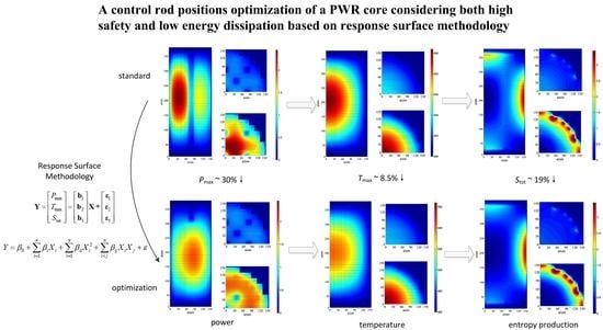
4.1. Standard Problem Solution

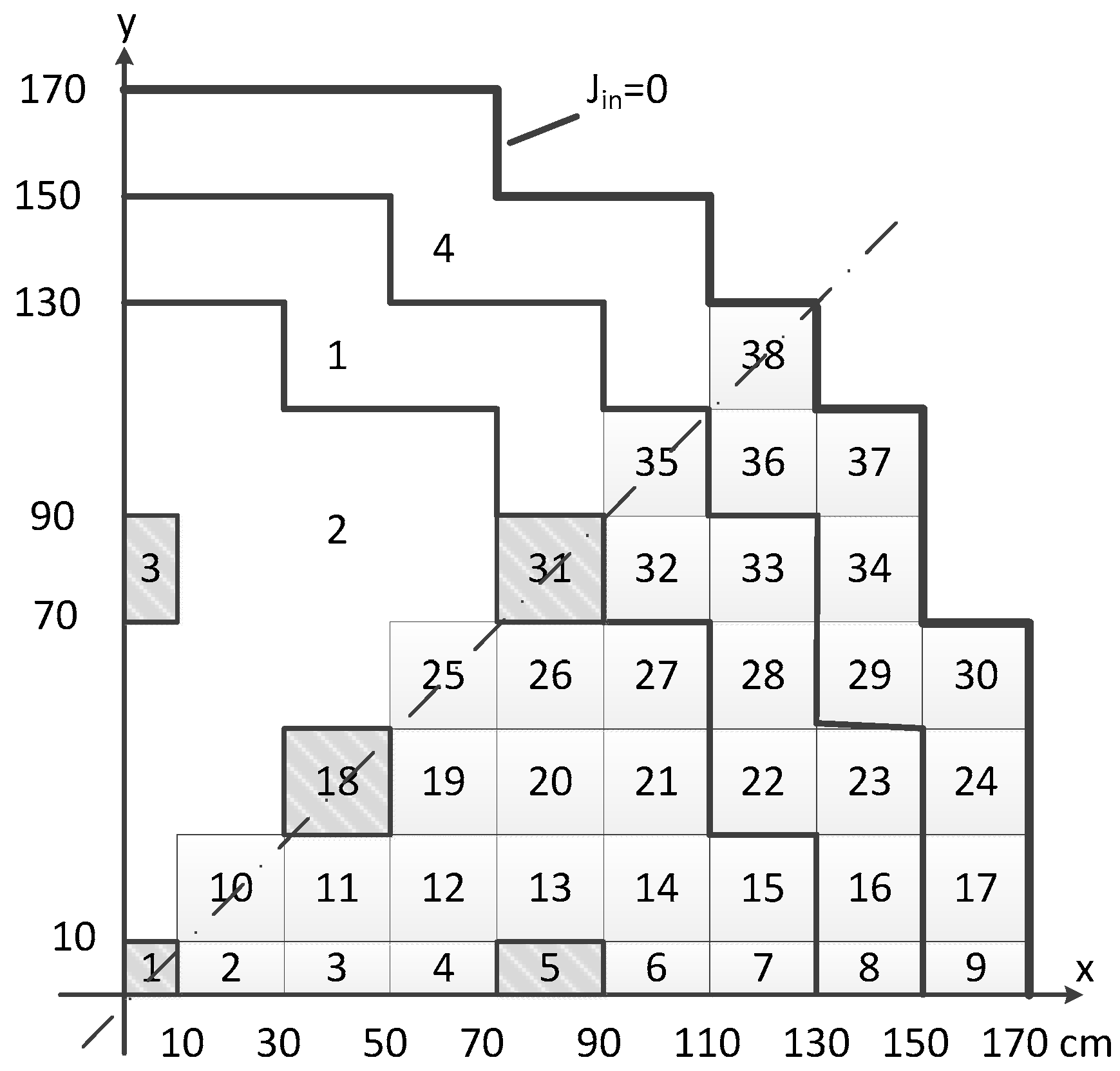
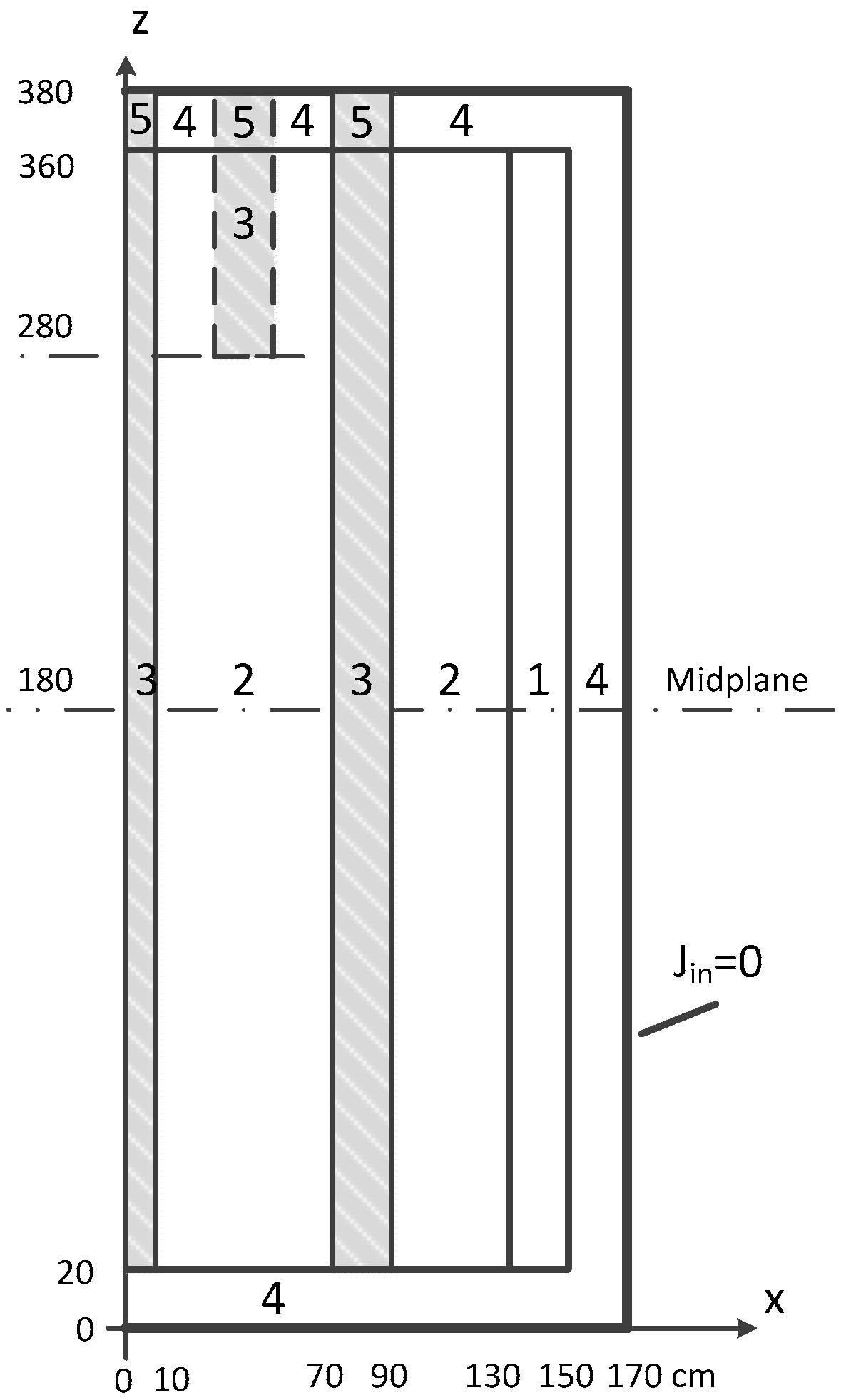
The control rod insertion positions shown in Figure 2 were chosen as the standard and reference solution. This example solution is the basis of the optimization. The neutron diffusion equations and heat transfer equations are all solved by FVM. In each calculation, the considered domain is one quarter of the whole core with reflective and non-return external boundaries. The convergence criterion is set as maximum relative flux change on each inner iteration = 10⁻¹⁰, maximum k_eff change on outer iteration = 10⁻⁶. Four groups of regular hexahedral meshes are taken into consideration. The mesh quantities and calculation results are given in

Table 3. Results on different mesh quantity.

No.	Mesh Quantity	keff	Error
1	17 × 17 × 19 (5491)	1.02904	-
2	34 × 34 × 38 (43,928)	1.02855	0.048%
3	51 × 51 × 57 (148,257)	1.02867	0.012%
4	68 × 68 × 76 (351,424)	1.02873	0.006%

. The error in Table 3 represents the relative error between using a mesh group and its further refinement.

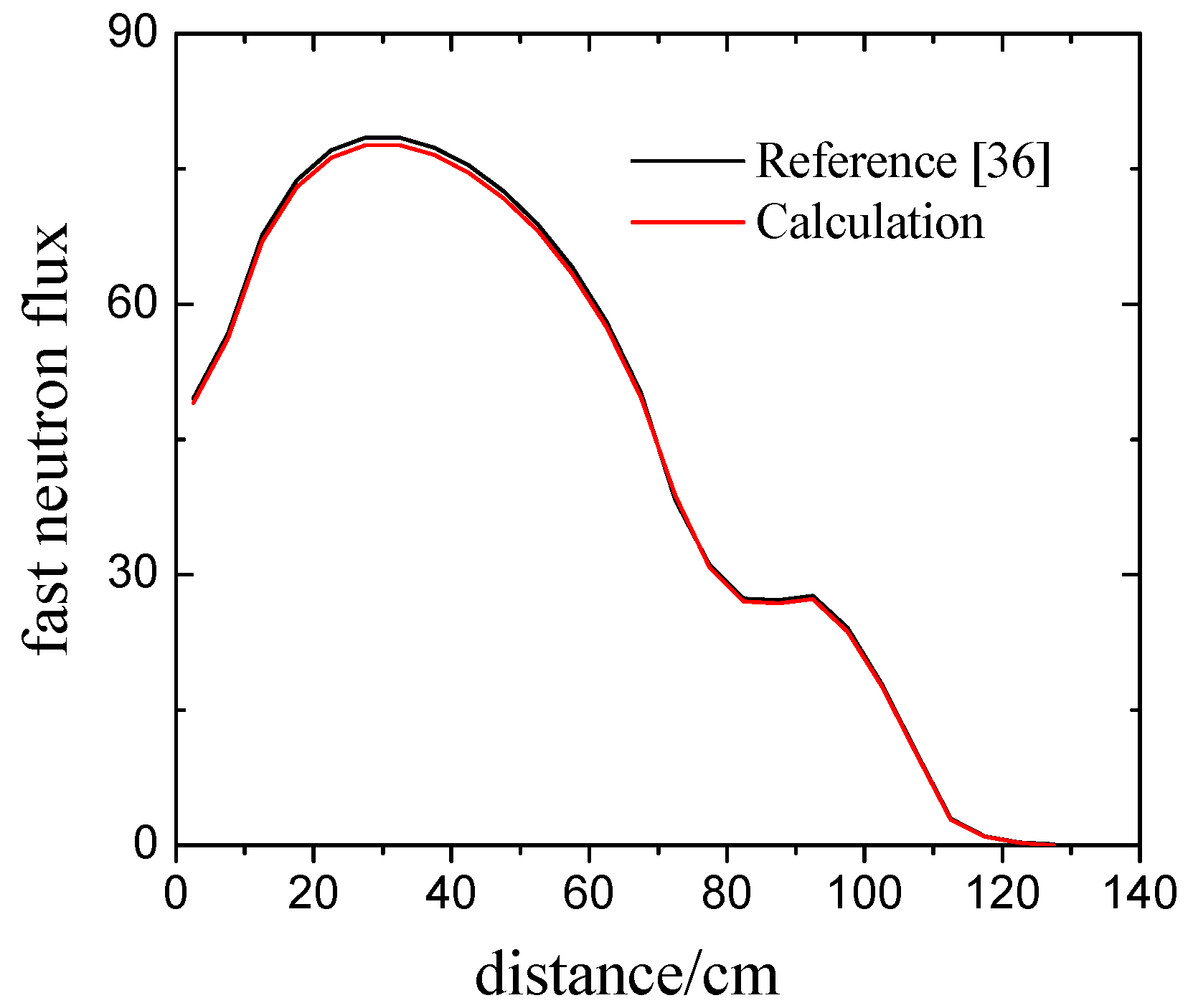
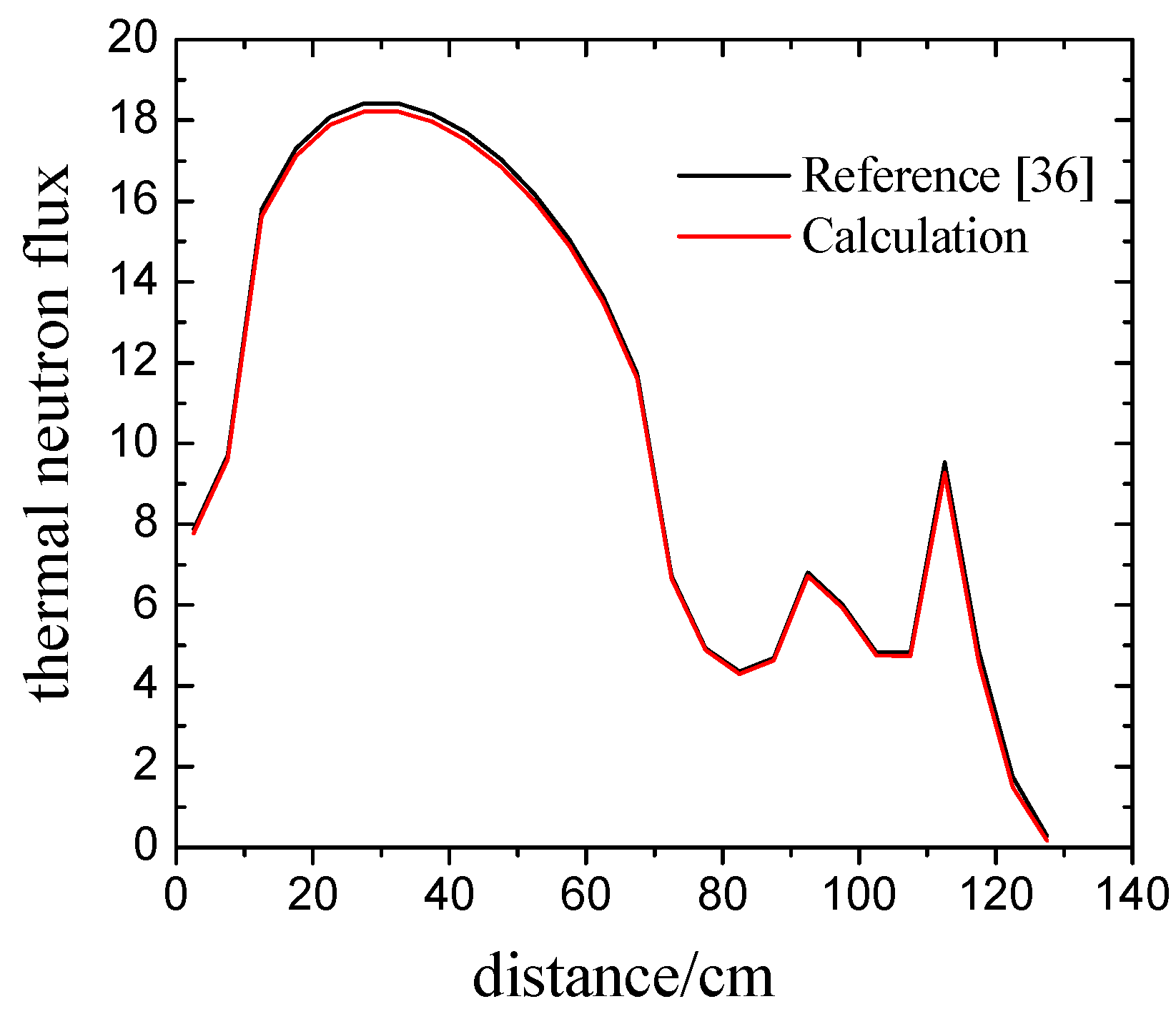
Considering both of the calculation accuracy and time cost, mesh No. 2 was selected to be applied for the next optimization scheme. This quantity of mesh is also used in [36], thus our neutron diffusion calculation results can be checked. The calculated k_eff is 1.02855 and the reference at the same mesh quantity is 1.02864, with the difference of 0.0087%. The results of fast and thermal neutron flux at the diagonal line on the x-y plane at the level of z = 195 cm are plotted in Figure 3 and Figure 4. A good match between calculated results and references can be seen.

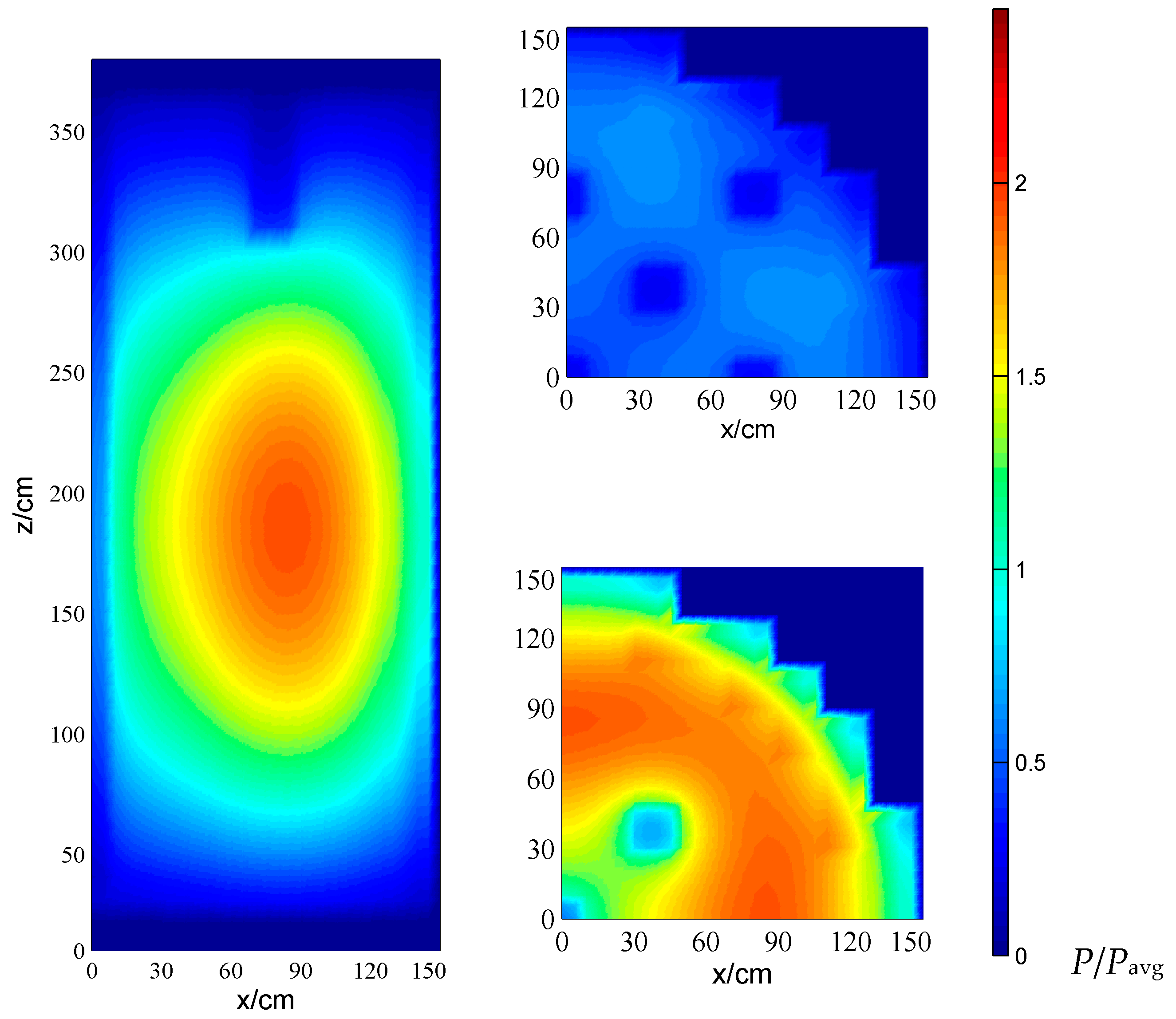
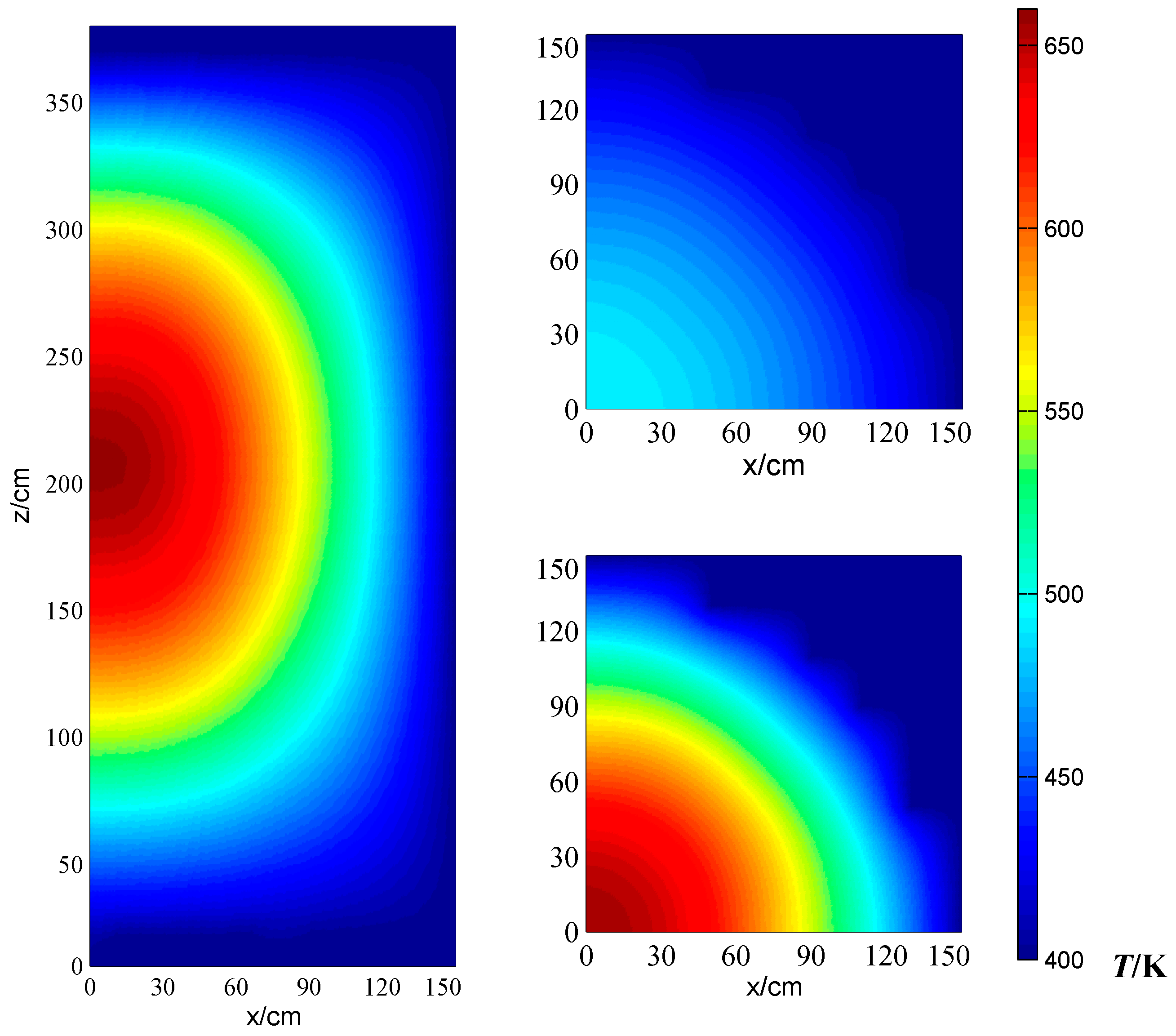
The calculation local power, temperature and entropy production results are plotted in Figure 5, Figure 6 and Figure 7. It can be seen in Figure 5 that the control rods have an obvious effect on the neutron fission power. Both the vertical and horizontal cross sections show significant decreases of local power depending on the control rod positions. The comparison of horizontal cross section at different z levels shows that the local power near the center of the core is higher than at the upper level, as expected. 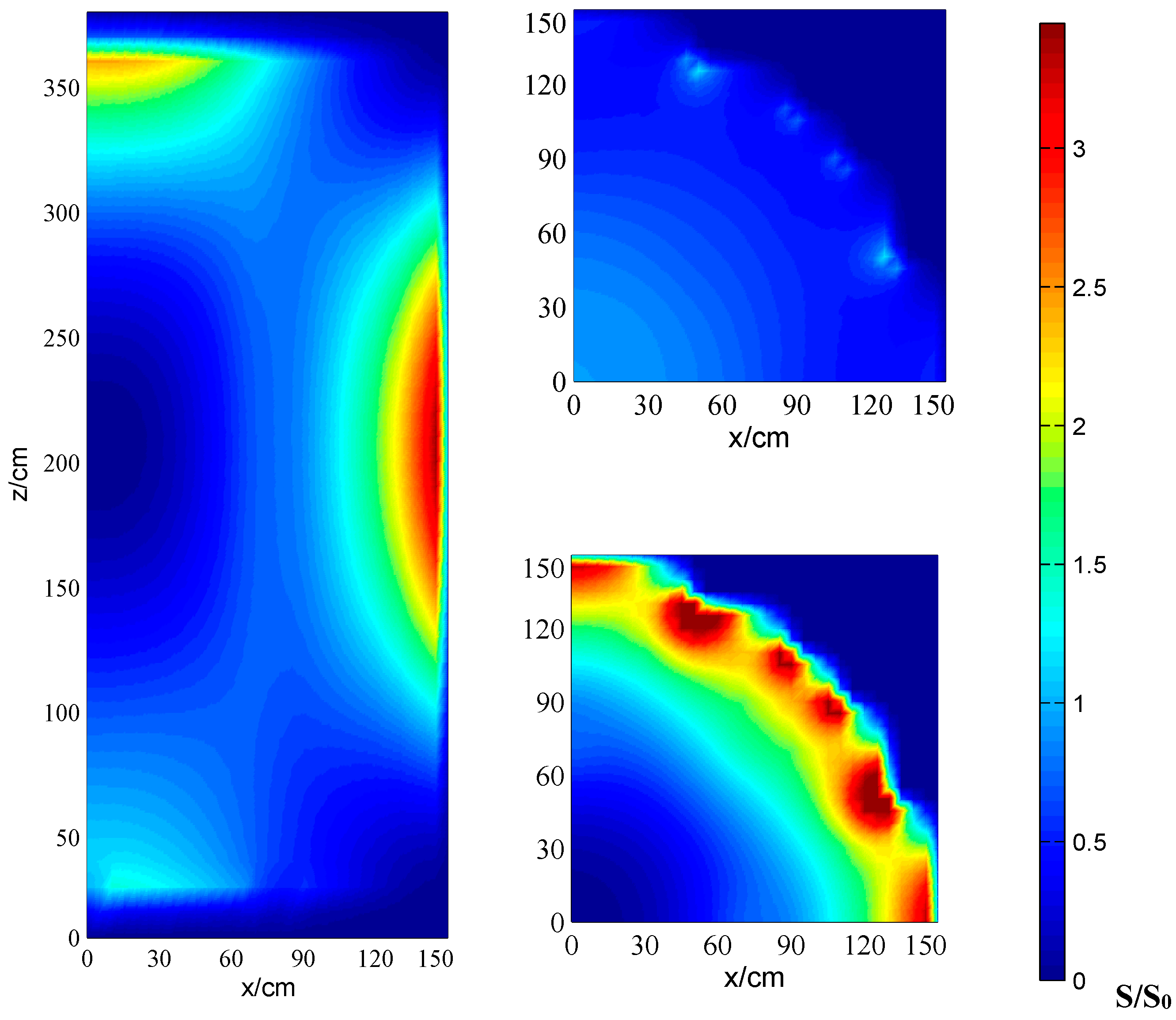Figure 6 shows that the regular temperature distribution is not as complex as the fission power distribution. It shows a continuous reduce from the core center to the edge. The control rod positions cannot be seen clearly in these temperature cloud pictures. The regular local entropy production distribution is far from the temperature distribution.

Figure 7 shows that the boundary centers of the reactor core are the peaks of the local entropy production, and the volume center of the reactor core is the valley of the local entropy production. The reason is that this core is symmetric at the vertical middle cross section, thus the middle cross section is heat insulated and the temperature gradient there is zero. The rapid decrease of temperature near the boundary center causes the entropy production peak.

In total, some lumped and feature parameters are selected to describe the thermal situation of the reactor core. These parameters are the power peak factor P_max, the maximum temperature T_max and the total entropy production S_tot. These parameters’ values are shown in

Table 4. Calculation results of standard problem.

Parameter	Pmax	Tmax	Stot
Value	2.5107	657.4	0.8021

.

4.2. Response Surface Design

The BBD is introduced to apply the RSM. The insert positions of control rods Z₁, Z₂, Z₃, Z₄ are the input independent variables, and the feature parameters P_max, T_max, S_tot are chosen as the response variables. The RSM can be written as follows:

$$Y=\left[\begin{array}{c}{P}_{\max }\\ T_{\max }\\ S_{\mathrm{tot}}\end{array}\right]=\left[\begin{array}{c}{b}_1\\ b_2\\ b_3\end{array}\right]X+\left[\begin{array}{c}{\mathsf{\epsilon }}_1\\ {\mathsf{\epsilon }}_2\\ {\mathsf{\epsilon }}_3\end{array}\right]$$

(17)

where:

$$X=\left[\begin{array}{lllllllllllllll}1\hfill & Z_1\hfill & Z_2\hfill & Z_3\hfill & Z_4\hfill & Z_1^2\hfill & Z_2^2\hfill & Z_3^2\hfill & Z_4^2\hfill & Z_1{Z}_2\hfill & Z_1{Z}_3\hfill & Z_1{Z}_4\hfill & Z_2{Z}_3\hfill & Z_2{Z}_4\hfill & Z_3{Z}_4\hfill \end{array}\right]$$

(18)

In order to establish the coefficient matrix b, several experiments should be performed. Section 4.1 presents an example of a numerical experiment. The input variables are [Z₁ Z₂ Z₃ Z₄] = [202802020], and the response result Y is given in Table 4. Using BBD to design the RSM for this problem, 29 groups of numerical experiments must be executed. The input and response variables are shown in

Table 5. Numerical experiments used to design response surface.

No.	Positions				Calculation Results			No.	Positions				Calculation Results
	Z1	Z2	Z3	Z4	Pmax	Tmax	Stot		Z1	Z2	Z3	Z4	Pmax	Tmax	Stot
1	360	190	20	190	3.258	681.4	0.8159	16	190	190	360	360	2.594	658	0.7794
2	190	190	190	190	3.24	690.7	0.8615	17	360	190	360	190	2.808	673.1	0.8231
3	20	190	190	360	2.445	641.4	0.7607	18	190	190	360	20	3.228	688.6	0.8565
4	360	20	190	190	2.211	633	0.7141	19	190	190	20	360	2.889	658.6	0.7531
5	190	20	190	20	2.696	649.8	0.7491	20	190	360	190	20	3.257	694.4	0.8805
6	190	190	190	190	3.24	690.7	0.8615	21	190	190	20	20	3.919	703.4	0.8588
7	190	20	20	190	2.052	610.4	0.6448	22	190	360	360	190	2.511	663.8	0.8186
8	190	190	190	190	3.24	690.7	0.8615	23	20	190	360	190	2.328	639.5	0.7644
9	190	360	190	360	2.624	663.7	0.7999	24	190	190	190	190	3.24	690.7	0.8615
10	190	20	190	360	2.071	619.4	0.6795	25	360	190	190	360	2.938	676	0.8196
11	20	190	190	20	2.919	668.8	0.8355	26	190	360	20	190	2.89	669.4	0.8045
12	360	190	190	20	3.649	709.8	0.9074	27	360	360	190	190	2.839	680.2	0.8497
13	190	20	360	190	2.026	622.4	0.7011	28	190	190	190	190	3.24	690.7	0.8615
14	20	360	190	190	2.332	645.7	0.7842	29	20	20	190	190	2.041	595.6	0.6406
15	20	190	20	190	2.486	637.9	0.7365	-	-	-	-	-	-	-	-

. The matrix b is obtained by Equation (17) and the fitting results are shown in

Table 6. Coefficients in the response surface.

Coefficient	b1	b2	b3	Coefficient	b1	b2	b3
β0	1.825872	573.3465	0.564135	β23	−3.10 × 10−6	−1.50 × 10−4	−3.60 × 10−7
β1	0.005768	0.374931	0.000685	β24	−7.00 × 10−8	−2.20 × 10−6	−9.50 × 10−8
β2	0.010037	0.628899	0.001546	Β34	3.42 × 10−6	1.23 × 10−4	2.48 × 10−7
β3	0.002126	0.207316	0.000692	β11	−1.00 × 10−5	−6.10 × 10−4	−1.10 × 10−6
β4	−0.00324	−0.1222	−0.00021	β22	−2.20 × 10−5	−1.19 × 10−4	−2.80 × 10−6
β12	2.91 × 10−6	−2.50 × 10−5	−6.90 × 10−8	β33	−7.10 × 10−6	−5.10 × 10−4	−1.50 × 10−6
β13	−2.50 × 10−6	−8.60 × 10−5	−1.80 × 10−7	β44	2.59 × 10−6	3.41 × 10−5	−1.10 × 10−7
β14	−2.10 × 10−6	−5.60 × 10−5	−1.10 × 10−7	-	-	-	-

.

The fitting results are usually evaluated by R-square. For this evaluation index, the closer to 1, the better result gained. The R-square value of the three response surface fitting is shown in

Table 7. R-square of response surface fitting.

Response	Pmax	Tmax	Stot
R-square	0.9495	0.9905	0.9892

.

It can be seen in Table 7 that, although T_max is a local feature, depending on its simple regular distribution, the R-square of its response surface is the highest. The second is S_tot since it is a total summary of local entropy production. It has the both global and local parameter features, so its sensitivity to the input variables is weaker than that of the local parameter. The R-square of the P_max response surface is not as fine as the others, due to the complex local power distribution. As these response surfaces are introduced to find out the direction of optimization, rather than obtain the exact solution, this level of fitting can also be applied.

4.3. Rod Position Optimization

In this section, a simple code is programmed to traverse all four input variable ranges in the definition domain, which is set as [30 cm, 300 cm]. The coefficients in Table 6 and Equation (18) are used in this code to obtain the approximate response results. The interval step of the input variables is set as 10 cm. In every traversal calculation, one evaluation index (P_max, T_max or S_tot) is selected as the optimization direction. The aim of optimization is to promote safety or reduce entropy dissipation, that is to say, P_max, T_max or S_tot should be reduced.

Although these three indexes are key metrics for a reactor core, the importance rankings are not at the same level for each of them. For every nuclear energy system, safety is always a seriously concerned for the public [42], and its status is higher than economical efficiency. T_max is the most obvious safety index, as the reactor materials may melt above a certain temperature limit, which would cause a serious accident. P_max is also a type of safety index, which is associated with the level of power flattening. A more flattened power distribution means a smoother reactor operation is expected. The last is the economical index S_tot, which represents the energy dissipation.

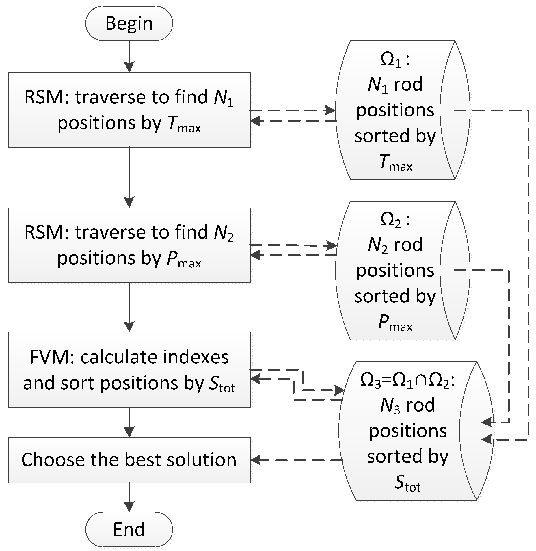
Therefore, our optimization procedure is: (1) use RSM to traverse all the control rod positions to find N₁ positions approaching the lowest T_max. The selected positions are put in set Ω₁; (2) Use RSM again to traverse all the positions in the definition domain to find N₂ positions approaching the lowest P_max and name the selected positions set as Ω₂; (3) Use FVM to obtain accurate indexes of position elements in Ω₃, Ω₃ = Ω₁ ∩ Ω₂, and sort them by S_tot. The best solution is chosen as the final optimization scheme. The flow diagram of this optimization procedure is shown in Figure 8.

In this scheme, a smaller N₁ or N₂ means a narrower search range, but the indexes may become closer to the limit. In this case, they are set as N₁ = N₂ = 10. Finally, eight groups of control rod positions are selected, which are listed in

Table 8. The selected control rod positions.

No.	Positions	Stot	Pmax	Tmax
1	[30 30 300 300]	0.6703	1.9408	600.47
2	[30 40 300 300]	0.6707	1.9418	600.58
3	[50 30 300 300]	0.6709	1.9433	600.64
4	[40 30 300 300]	0.6710	1.9439	600.66
5	[30 30 290 300]	0.6724	1.9602	601.19
6	[40 30 300 290]	0.6731	1.9550	601.25
7	[30 30 300 290]	0.6733	1.9561	601.30
8	[30 30 300 280]	0.6752	1.9674	601.86

.

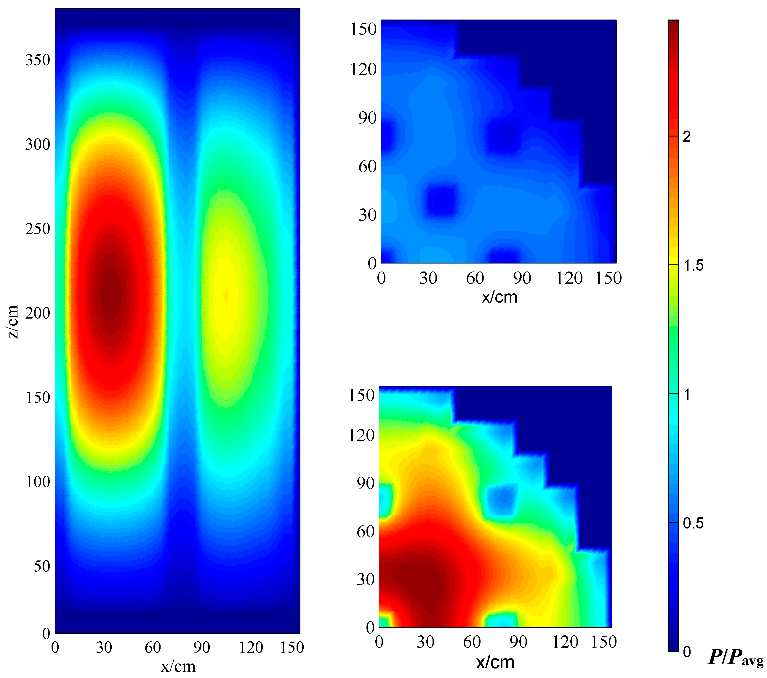
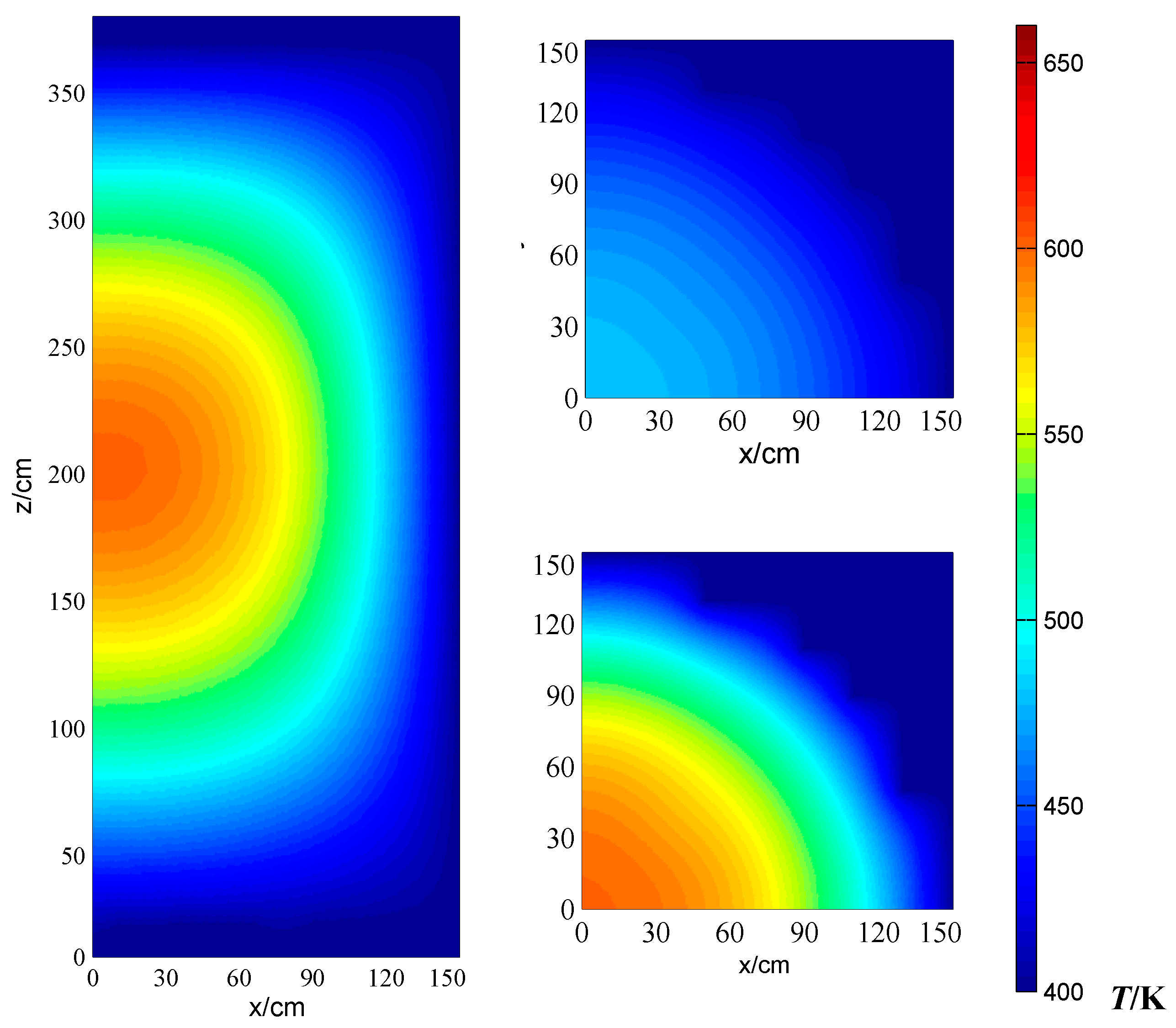
It can be seen in Table 8 that the safety and entropy index will reach optimization when the central control rods are inserted deeply and the peripheral control rods are inserted shallowly. In the calculation series, it can be found that when the input rod positions are [30 30 300 300], the P_max, T_max and S_tot reach the minimum, which means that both the power and temperature are flatter, and the energy dissipation reaches the minimum. In order to observe the physical field in depth, the distributions of local power, temperature and local entropy production are illustrated in Figure 9, Figure 10 and Figure 11.

The cloud pictures Figure 9 and Figure 11 share the same colorbar scale as Figure 5, Figure 6 and Figure 7, respectively. Thus the differences between these two groups can be clearly observed. Comparing Figure 9 with Figure 5, it can be found that the power flattening effect is better after the control rod adjustment. 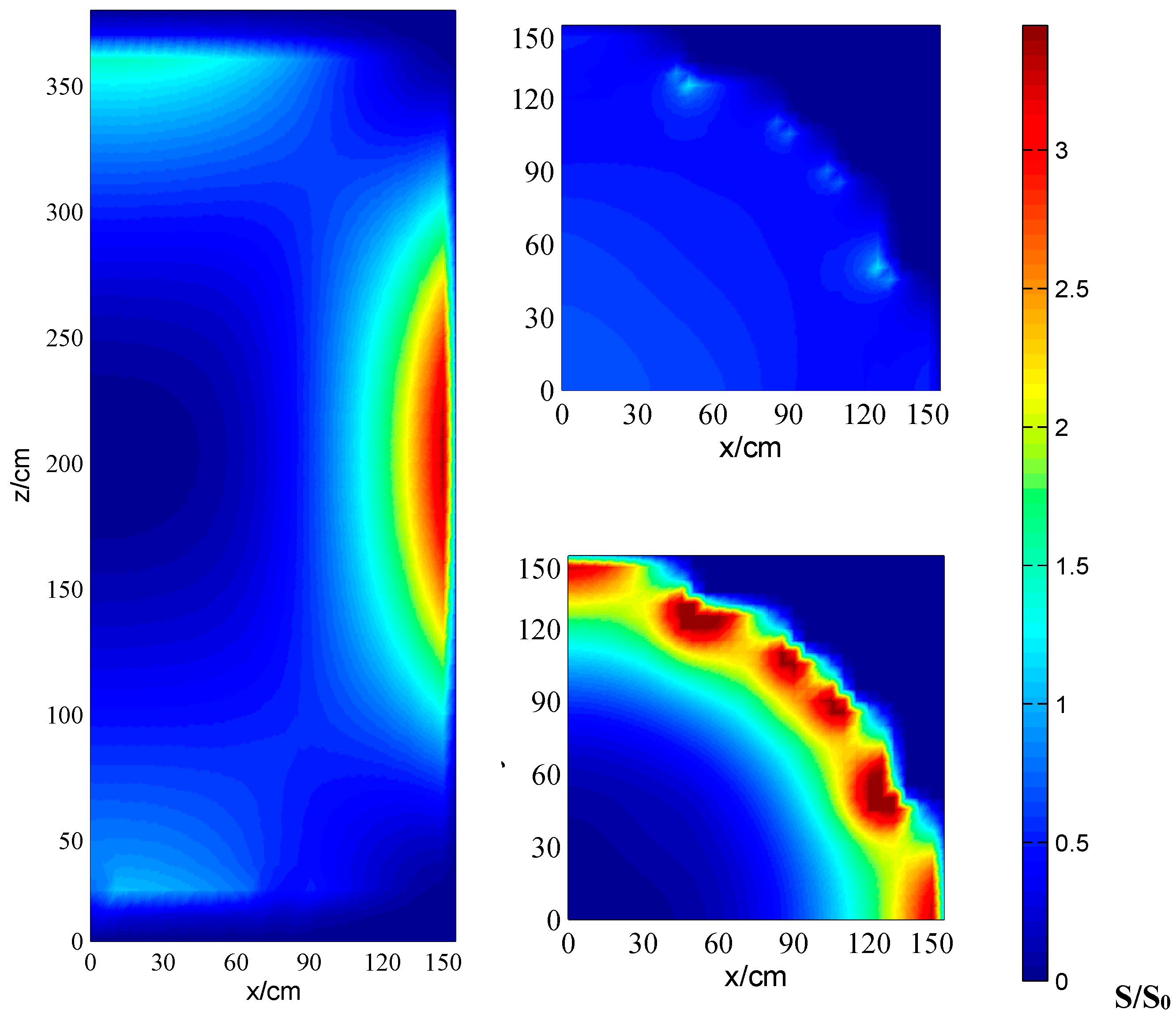The central control rod has an obvious influence on the power distribution, which causes a power valley at the core center, so the temperature at the center line of x = y = 0, is not so high as the temperature in the standard problem, which can be seen in Figure 6 and Figure 10. The distribution of local entropy production is similar between Figure 7 and Figure 11, but the entropy production values are reduced after control rod adjustment.

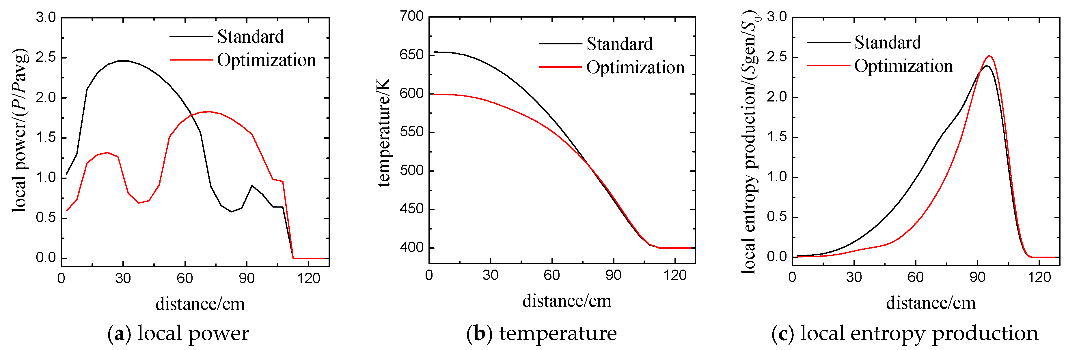
In order to show some details of the optimization results, the local power, temperature and local entropy production at the diagonal line on midplane are shown in Figure 12. It can be seen in Figure 12a that the local power decreases near the core center and a power valley forms between the distance of 40 cm and 50 cm, as the control rods in FA.1 and FA.18 are inserted deeply. At the same time, with the control rods in FA.5 and FA.31 rise, the local power of the optimization scheme is higher than that of the standard problem in the distance range of [65 cm, 110 cm]. As a result, local power is flatter than in the standard problem and the power peak factor is reduced. For the temperature distribution, as shown in Figure 12b, the temperature and its gradient are reduced near the core center while a little increase is noted near the core boundary, which matches the local power distribution. The change of temperature gradient causes a lower local entropy production near the core center and the one higher near the core boundary, which is shown in Figure 12c.

As a result, the evaluation indexes of the standard problem and optimization scheme are listed in

Table 9. Comparison between calculation results.

Parameter	Standard Problem	Optimization Scheme	Decrease
Pmax	2.5107	1.9408	23%
Tmax	657.4	600.47	8.7%
Stot	0.8021	0.6703	16%

. An obvious decrease can be seen, which is satisfactory for the optimization.

5. Conclusions

In this paper, a typical PWR reactor core based on the 3D-IAEA problem is taken to be analysed. The neutron flux field, temperature and local entropy production distribution in this reactor core are calculated by FVM. The calculation results are illustrated in cloud pictures in order to observe them clearly. For evaluating the safety and energy dissipation, three characteristics are selected as evaluation indexes, which are the power peak factor P_max, the maximum temperature T_max, and the total entropy production S_tot. Then the RSM is introduced to optimize the control rod insertion positions in order to get a lower P_max, T_max and S_tot, which means higher safety and lower energy dissipation. Three directions of optimization are taken, and a final optimization scheme is obtained. The comparison of cloud pictures between the standard problem and optimization scheme shows that the central control rod has a great influence on the power distribution. In total, P_max, T_max and S_tot are reduced by 23%, 8.7% and 16% after the adjustment of the control rod insert positions, which is satisfactory. RSM may be a quick and useful method in reactor optimization.

References

1. Niu, S.; Liu, Y.; Ding, Y.; Qu, W. China’s energy systems transformation and emissions peak. Renew. Sustain. Energy Rev. 2016, 58, 782–795. [Google Scholar] [CrossRef]
2. Guo, X.; Guo, X. Nuclear power development in China after the restart of new nuclear construction and approval: A system dynamics analysis. Renew. Sustain. Energy Rev. 2016, 57, 999–1007. [Google Scholar] [CrossRef]
3. Shi, H.Y.; Song, H.T. Applying the real option approach on nuclear power project decision making. Energy Procedia 2013, 39, 193–198. [Google Scholar] [CrossRef]
4. Weisman, J. Elements of Nuclear Reactor Design, 2nd ed.; Robert, E., Ed.; Krieger Publishing Co. Inc.: Malabar, FL, USA, 1983. [Google Scholar]
5. Duderstadt, J.J.; Hamilton, L.J. Nuclear Reactor Analysis; John Wiley and Sons Inc.: New York, NY, USA, 1976. [Google Scholar]
6. Nahla, A.A. Efficient computational system for transient neutron diffusion model via finite difference and theta methods. Ann. Nucl. Energy 2015, 89, 28–37. [Google Scholar] [CrossRef]
7. Pazirandeh, A.; Jalili, B.M.H.; Abadi, P. Finite difference method for solving neutron diffusion equation in hexagonal geometry. In Proceedings of the International Conference Nuclear Energy for New Europe, Bled, Slovenia, 14–17 September 2009.
8. Harvie, D.J.E. An implicit finite volume method for arbitrary transport equations. ANZIAM J. 2010, 52, C1126–C1145. [Google Scholar] [CrossRef]
9. Bernal, A.; Roman, J.E.; Miro, R.; Verdú, G. Assembly discontinuity factors for the neutron diffusion equation discretized with the finite volume method application to BWR. Ann. Nucl. Energy 2016, 97, 76–85. [Google Scholar] [CrossRef]
10. Theler, G. Unstructured grids and the multigroup neutron diffusion equation. Sci. Technol. Nucl. Instrall. 2013, 2013, 333–339. [Google Scholar] [CrossRef]
11. Ge, J.; Zhang, D.; Tian, W.; Wang, K.; Qiu, S.; Su, G.H. Steady and transient solutions of neutronics problems based on finite volume method (FVM) with a CFD code. Prog. Nucl. Energy 2015, 85, 366–374. [Google Scholar] [CrossRef]
12. Hosseini, S.A. Development of galerkin finite element method three-dimensional computational code for the on diffusion equation with unstructured tetrahedron elements. Nucl. Eng. Technol. 2015, 48, 43–54. [Google Scholar] [CrossRef]
13. Eleodor, N.; Farzad, R. A heterogeneous finite element method in diffusion theory. Ann. Nucl. Energy 2003, 30, 317–347. [Google Scholar]
14. Vidal-Ferrandiz, A.; Fayez, R.; Ginestar, D.; Verdú, G. Moving meshes to solve the time-dependent neutron diffusion equation in hexagonal geometry. J. Comput. Appl. Math. 2016, 291, 197–208. [Google Scholar] [CrossRef]
15. Bejan, A. A study of entropy generation in fundamental convective heat transfer. J. Heat Transf. 1979, 101, 718–725. [Google Scholar] [CrossRef]
16. Bejan, A. Entropy Generation through Heat and Fluid Flow. J. Appl. Mech. 1983, 50, 475. [Google Scholar] [CrossRef]
17. Bejan, A. Advanced Engineering Thermodynamics, 2nd ed.; Wiley: New York, NY, USA, 1997. [Google Scholar]
18. Bejan, A. Entropy Generation Minimization; CRC Press: New York, NY, USA, 1996. [Google Scholar]
19. Ibáñez, G.; Cuevas, S.; Haro, M.L.D. Minimization of entropy generation by asymmetric convective cooling. Int. J. Heat Mass Transf. 2003, 46, 1321–1328. [Google Scholar] [CrossRef]
20. Makinde, D.; Aziz, A. Analysis of entropy generation and thermal stability in a long hollow cylinder with asymmetry convective cooling. Heat Mass Transf. 2011, 47, 1407–1415. [Google Scholar] [CrossRef]
21. Aziz, A.; Khan, W.A. Entropy generation in an asymmetrically cooled slab with temperature-dependent internal heat generation. Heat Trans. Res. 2012, 41, 260–271. [Google Scholar] [CrossRef]
22. Malvandi, A.; Ganji, D.D.; Hedayati, F.; Yousefi Rad, E. An analytical study on entropy generation of nanofluids over a flat plate. Alex. Eng. J. 2013, 52, 595–604. [Google Scholar] [CrossRef]
23. Torabi, M.; Zhang, K. Classical entropy generation analysis in cooled homogenous and functionally graded material slabs with variation of internal heat generation with temperature, and convective–radiative boundary conditions. Energy 2014, 65, 387–397. [Google Scholar] [CrossRef]
24. Ivanov, K.; Avramova, M. Challenges in coupled thermal-hydraulics and neutronics simulations for LWR safety analysis. Energy 2007, 34, 501–513. [Google Scholar] [CrossRef]
25. Sjenitzer, B.L.; Hoogenboom, J.E.; Escalante, J.J.; Espinoza, V.S. Coupling of dynamic Monte Carlo with thermal-hydraulic feedback. Ann. Nucl. Energy 2015, 76, 27–39. [Google Scholar] [CrossRef]
26. Knoll, D.A.; Keyes, D.E. Jacobian-free Newton-Krylov methods: A survey of approaches and applications. J. Comput. Phys. 2004, 193, 357–397. [Google Scholar] [CrossRef]
27. Song, H.; Luo, R.; Wan, J.; Li, S.; Zhao, F. Development of a novel 1D coupled neutronics/thermal-hydraulics code and its verification on PWR rod ejection accident benchmark. Prog. Nucl. Energy 2016, 92, 197–210. [Google Scholar] [CrossRef]
28. Bezerra, M.A.; Santelli, R.E.; Oliveira, E.P.; Villar, L.S.; Escaleira, L.A. Response surface methodology (RSM) as a tool for optimization in analytical chemistry. Talanta 2008, 76, 965–977. [Google Scholar] [CrossRef] [PubMed]
29. Gilmour, S.G. Response surface designs for experiments in bioprocessing. Biometrics 2006, 62, 323–331. [Google Scholar] [CrossRef] [PubMed]
30. Kalil, S.J.; Maugeri, F.; Rodrigues, M.I. Response surface analysis and simulation as a tool for bioprocess design and optimization. Process Biochem. 2000, 36, 539–550. [Google Scholar] [CrossRef]
31. Rajashekhar, M.R.; Ellingwood, B.R. A new look at the response surface approach for reliability analysis. Struct. Saf. 1993, 12, 205–220. [Google Scholar] [CrossRef]
32. Bucher, C.G.; Bourgund, U. A fast and efficient response surface approach for structural reliability problems. Struct. Saf. 1990, 7, 57–66. [Google Scholar] [CrossRef]
33. D’Archivio, A.A.; Maggi, M.A. Investigation by response surface methodology of the combined effect of pH and composition of water-methanol mixtures on the stability of curcuminoids. Food Chem. 2017, 219, 414–418. [Google Scholar] [CrossRef] [PubMed]
34. Espadabellido, E.; Ferreirogonzalez, M.; Carrera, C.; Palma, M.; Barroso, C.G.; Barbero, G.F. Optimization of the ultrasound- assisted extraction of anthocyanins and total phenolic compounds in mulberry (Morus nigra) pulp. Food Chem. 2016, 219, 23–32. [Google Scholar] [CrossRef] [PubMed]
35. Wang, Y.; Gao, Y.; Ding, H.; Liu, S.; Han, X.; Gui, J.; Liu, D. Subcritical ethanol extraction of flavonoids from Moringa oleifera leaf and evaluation of antioxidant activity. Food Chem. 2017, 218, 152–158. [Google Scholar] [CrossRef] [PubMed]
36. Argonne Code Center: Benchmark Problem Book. ANL-7416 (Supplement 2). Available online: https://www.osti.gov/scitech/servlets/purl/5037820 (accessed on 8 February 2017).
37. Stacey, W.M. Nuclear Reactor Physics; Wiley: New York, NY, USA, 2001. [Google Scholar]
38. Bernal, A.; Roman, J.E.; Miró, R.; Ginestar, D. Development of a finite volume inter-cell polynomial expansion method for the neutron diffusion equation. J. Nucl. Sci. Technol. 2016, 53, 1212–1223. [Google Scholar] [CrossRef]
39. Chen, W.; Yu, L.; Hao, J. Thermal-Hydraulics of Nuclear Power Facilities; Atomic Press: Beijing, China, 2012. [Google Scholar]
40. Aslan, N.; Cebeci, Y. Application of Box-Behnken design and response surface methodology for modeling of some Turkish coals. Fuel 2007, 86, 90–97. [Google Scholar] [CrossRef]
41. Kincl, M.; Turk, S.; Vrecer, F. Application of experimental design methodology in development and optimization of drug release method. Int. J. Pharm. 2005, 291, 39–49. [Google Scholar] [CrossRef] [PubMed]
42. Lake, J.A. The fourth generation of nuclear power. Prog. Nucl. Energy 2002, 40, 301–307. [Google Scholar] [CrossRef]
Figure 1. Horizontal cross section of the 3D-IAEA problem.
Entropy 19 00063 g001
Figure 2. Vertical cross section of the 3D-IAEA problem.
Entropy 19 00063 g002
Figure 3. Fast neutron flux at the diagonal line at the level of z = 195 cm.
Entropy 19 00063 g003
Figure 4. Thermal neutron flux at the diagonal line at the level of z = 195 cm.
Entropy 19 00063 g004
Figure 5. Local power distribution of standard problem (left: vertical cross section cloud picture at y = 0; right-top: horizontal cross section cloud picture at z = 315 cm; right-bottom: horizontal cross section cloud picture at z = 195 cm. Pavg represents the average local power of standard problem).
Entropy 19 00063 g005
Figure 6. Temperature distribution of standard problem (left: vertical cross section cloud picture at y = 0; right-top: horizontal cross section cloud picture at z = 315 cm; right-bottom: horizontal cross section cloud picture at z = 195 cm).
Entropy 19 00063 g006
Figure 7. Local entropy production distribution of standard problem (left: vertical cross section cloud picture at y = 0; right-top: horizontal cross section cloud picture at z = 315 cm; right-bottom: horizontal cross section cloud picture at z = 195 cm. S0 represents the average local entropy production of standard problem).
Entropy 19 00063 g007
Figure 8. Flow diagram of optimization procedure.
Entropy 19 00063 g008
Figure 9. Local power distribution of optimization scheme (left: vertical cross section cloud picture at y = 0; right-top: horizontal cross section cloud picture at z = 315 cm; right-bottom: horizontal cross section cloud picture at z = 195 cm. Pavg represents the average local power of standard problem).
Entropy 19 00063 g009
Figure 10. Temperature distribution of optimization scheme (left: vertical cross section cloud picture at y = 0; right-top: horizontal cross section cloud picture at z = 315 cm; right-bottom: horizontal cross section cloud picture at z = 195 cm).
Entropy 19 00063 g010
Figure 11. Local entropy production distribution of optimization scheme (left: vertical cross section cloud picture at y = 0; right-top: horizontal cross section cloud picture at z = 315 cm; right-bottom: horizontal cross section cloud picture at z = 195 cm. S0 represents the average local entropy production of standard problem).
Entropy 19 00063 g011
Figure 12. Local power, temperature and local entropy production of the standard problem and optimization scheme at the diagonal line on the midplane (the level of z = 195 cm).
Entropy 19 00063 g012