A Risk-Free Protection Index Model for Portfolio Selection with Entropy Constraint under an Uncertainty Framework

Abstract

This paper aims to develop a risk-free protection index model for portfolio selection based on the uncertain theory. First, the returns of risk assets are assumed as uncertain variables and subject to reputable experts’ evaluations. Second, under this assumption, combining with the risk-free interest rate we define a risk-free protection index (RFPI), which can measure the protection degree when the loss of risk assets happens. Third, note that the proportion entropy serves as a complementary means to reduce the risk by the preset diversification requirement. We put forward a risk-free protection index model with an entropy constraint under an uncertainty framework by applying the RFPI, Huang’s risk index model (RIM), and mean-variance-entropy model (MVEM). Furthermore, to solve our portfolio model, an algorithm is given to estimate the uncertain expected return and standard deviation of different risk assets by applying the Delphi method. Finally, an example is provided to show that the risk-free protection index model performs better than the traditional MVEM and RIM.

1. Introduction

Portfolio selection focuses on the optimal allocation of one’s wealth to obtain maximum profitable return under minimum risk control. Since Markowitz [1] first proposed the classic mean-variance model (MVM), many researchers have suggested new methods or elements to get numerous variants of the MVM for portfolio selection (e.g., minimum-variance model [2], mean-variance-skewness model [3], mean-semivariance model [4]). Their research can be regarded as the extension to the classic portfolio theory which is based on probability and statistics theory. The security returns are all assumed to be random variables and their expected value and variance are obtained from the sample of available historical data. Considering the complexity of the security market in the real world, the non-uniqueness of randomness as a kind of uncertainty and the lack of enough historical data to reflect the future performances of security returns in some real life cases, many scholars began to regard security returns as fuzzy variables which rely on experienced experts’ evaluations instead of historical data. Thus, fuzzy portfolio optimization theory is developed and has been mainly studied based on following three methods: (i) Fuzzy set theory [5]; (ii) Possibility measure [6,7]; (iii) Credibility measure [8,9,10].

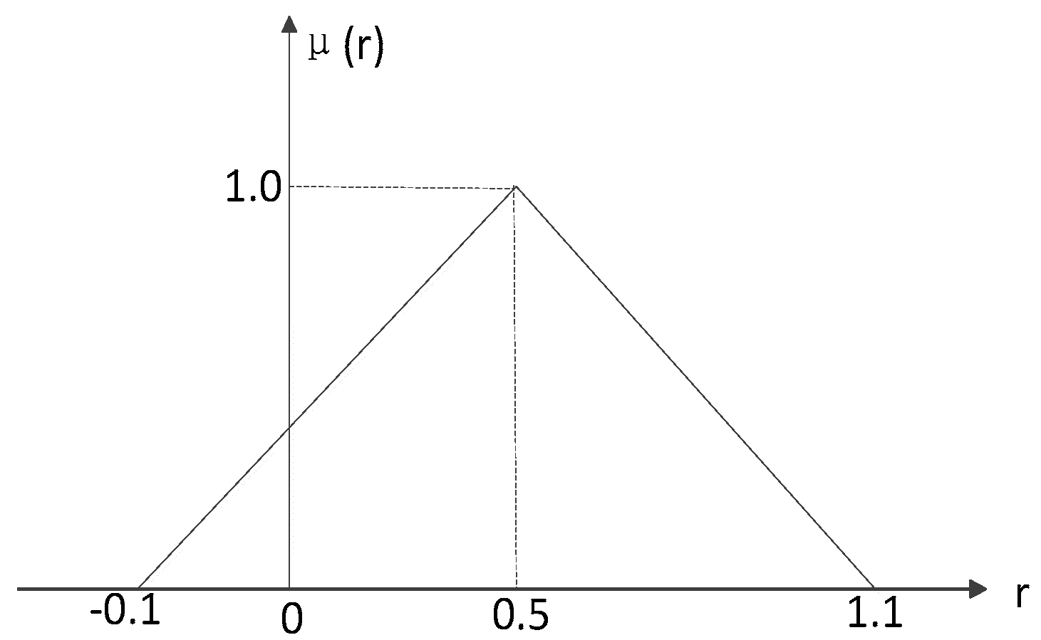
However, paradoxes arise when fuzzy variables are utilized to describe the subjective estimations of security returns in the above three methods [11]. For instance, if a security return is regarded as a fuzzy variable, then it can be characterized by a membership function. We suppose that a security return is the triangular fuzzy variable $\mathsf{\xi }=(-0.1,0.5,1.1)$ (see Figure 1). Based on the membership function, it is easy to obtain that $\mathrm{P}\mathrm{o}\mathrm{s}\{\mathsf{\xi }=0.5\}=1$ (or $\mathrm{Cr}\{\mathsf{\xi }=0.5\}=0.5$), which means that the security return is exactly 0.5 with belief degree 1 in possibility measure (or 0.5 in credibility measure). However, this is unreasonable because the degree belief of exactly 0.5 should be almost zero. In addition, we also get from the possibility theory that $\mathrm{P}\mathrm{o}\mathrm{s}\{\mathsf{\xi }\ne 0.5\}=\mathrm{P}\mathrm{o}\mathrm{s}\{\mathsf{\xi }=0.5\}=1$ (or $\mathrm{Cr}\{\mathsf{\xi }\ne 0.5\}=\mathrm{Cr}\{\mathsf{\xi }=0.5\}=0.5$. It implies that the two events of the return being exactly 0.5 and not being exactly 0.5 have the same degree belief both in possibility measure and credibility measure, and they are equally likely to happen. This conclusion is contradictory and unacceptable to our judgment.

To deal with the above situation, Liu [12,13,14,15] proposed an uncertain measure and further developed the uncertainty theory, which has been used in various areas (e.g., insurance, medical care, environment and education) especially in the study of portfolio optimization [16,17,18,19]. Qin, et al. [20] first studied mean-variance model in the uncertain environment. Zhu [21] considered a continuous-time uncertain portfolio optimization problem. Liu and Qin [22] proposed a mean semi-absolute deviation model for uncertain portfolio selection. Different from the above studies on risk measurement, some scholars took the risk-free interest rate into consideration in the uncertain portfolio optimization. Huang [23] first put forward a risk index model, Huang and Qiao [24] modeled the multi-period problem, Huang and Ying [11] further considered the portfolio adjusting problem. These studies proved that the above-mentioned paradoxes can be solved when the uncertain variable is used to describe human imprecise estimations of security returns [11,24].

However, we find that these researchers usually focused on the weight of risk assets for uncertain portfolio selection problem and ignored the protective screening function of risk-free asset. As a result, the capital allocation is usually too centralized or decentralized. In this paper, we study the portfolio selection problem under the framework of the uncertainty theory. In particular, we extend the work of Huang, et al. [11,23,24] by proposing a risk-free protection index model with entropy constraint for portfolio selection problem. Firstly, to introduce the protective screening function of risk-free asset in guaranteeing the expected return of portfolio selection as the loss of risk assets happens at a certain confidence level, we put forward a risk-free protection index (RFPI). Secondly, considering that the Mean-variance selection framework without entropy constraint may result in concentrative allocation, we further add proportion entropy constraint to the RFPI model to meet the preset diversification requirement, which can prevent the concentrative allocation. Finally, we propose a risk-free protection index model with proportion entropy constraint for portfolio selection problem under uncertainty framework. The RFPI model can evaluate the protection made by risk-free asset when the risk assets happen to lose at a certain confidence level, i.e., it can measure the protective effect of risk-free asset on risk assets.

The rest of the paper is organized as follows: Section 2 introduces the knowledge about uncertain variables and entropy constraint in finance. In Section 3, we first present RIM for uncertain portfolio and the MVEM for diversified fuzzy portfolio. Then we further propose a risk-free protection index model with entropy constraint in uncertainty environment and give an algorithm to solve the portfolio selection model. Illustrative example is given in Section 4. Section 5 draws the conclusion.

2. Knowledge about Uncertain Variables and the Entropy Constraint

To use uncertain variables to describe the security returns and consider the portfolio selection problem with an entropy constraint, this section first introduces some necessary knowledge about uncertain variables, and then presents an entropy constraint to finance.

2.1. The Expected Value, Variance and Distribution of an Uncertain Variable

Liu [12,13] presented an uncertain variable and an uncertain measure. We suppose that $\mathsf{\Gamma }$ is a nonempty set, $\mathsf{\zeta }$ is a $\mathsf{\sigma }$-algebra over $\mathsf{\Gamma }$, each element $\mathsf{\Lambda }\in \mathsf{\zeta }$ is an event, and $M\left\{\mathsf{\Lambda }\right\}$ is the occurrence possibility measure of $\mathsf{\Lambda }$. The function $M$ is called an uncertain measure if it satisfies four axioms:

(i)

Axiom 1: (Normality) $M\left\{\mathsf{\Gamma }\right\}=1$;

(ii)

Axiom 2: (Self-duality) $M\left\{\mathsf{\Lambda }\right\}+M\left\{{\mathsf{\Lambda }}^c\right\}=1$;

(iii)

Axiom 3: (Countable subadditivity) $M\left\{\underset{i=1}{\overset{\infty }{\cup }}{\mathsf{\Lambda }}_i\right\}\le {\displaystyle \sum _{i=1}^{\infty }M\left\{{\mathsf{\Lambda }}_i\right\}}$ for every event $\left\{{\mathsf{\Lambda }}_i\right\}$;

(iv)

Axiom 4: (Product measure) Let $({\mathsf{\Gamma }}_k,{\mathsf{\zeta }}_k,M_k)$ be uncertain spaces for $k=1,2,\cdots ,n$, then product uncertain measure is $M=M_1\wedge M_2\wedge \cdots \wedge M_n$.

Let $M$ be an uncertain measure. The triplet $(\mathsf{\Gamma },\mathsf{\zeta },M)$ is called an uncertainty space. An uncertain variable is a measurable function $\mathsf{\xi }$:$(\mathsf{\Gamma },\mathsf{\zeta },M)\to \Re$, i.e., the Borel set $\mathrm{B}$:$\text{{}\mathsf{\xi }\in B\}=\{\mathsf{\gamma }\in \mathsf{\Gamma }|\mathsf{\xi }(\mathsf{\gamma })\in \mathrm{B}\text{}}$ is an event. Then the uncertain distribution is defined as $\mathsf{\Phi }(x)=M\{\mathsf{\xi }\le x\}$, $\mathsf{\Phi }:\Re \to [0,1]$.

The expected value is defined as

$$\mathrm{E}\left[\mathsf{\xi }\right]={\displaystyle {\int }_0^{\infty }M\left\{\mathsf{\xi }\ge r\right\}}dr-{\displaystyle {\int }_{-\infty }^{0}M\left\{\mathsf{\xi }\le r\right\}}dr.$$

(1)

and its variance is defined as

$$V[\mathsf{\xi }]=E[{(\mathsf{\xi }-E[\mathsf{\xi }])}^2].$$

(2)

If $\mathsf{\xi }$ and $\mathsf{\eta }$ are independent uncertain variables with finite expected values, then it holds that

$$E[a\mathsf{\xi }+b\mathsf{\eta }]=aE[\mathsf{\xi }]+bE[\mathsf{\eta }],\mathrm{for}\forall a,b\in \Re .$$

(3)

An uncertain variable $\mathsf{\xi }$ is named as the normal uncertain variable if it satisfies

$$\mathsf{\Phi }\left(x\right)={\left[1+\exp \left(\frac{\mathsf{\pi }\left(\mathrm{e}-x\right)}{\sqrt{3}\mathsf{\sigma }}\right)\right]}^{-1},x\in \Re ,$$

(4)

which is denoted by $N\left(e,\mathsf{\sigma }\right)$ with the mean value $e$ and standard variance σ. The inverse function can be written as [13]

$${\mathsf{\Phi }}^{-1}(\mathsf{\alpha })=e+\frac{\sqrt{3}\mathsf{\sigma }}{\mathsf{\pi }}\ln \frac{\mathsf{\alpha }}{1-\mathsf{\alpha }},$$

(5)

where $\mathsf{\alpha }\in (0,1)$ and ${\mathsf{\Phi }}^{-1}(\mathsf{\alpha })$ is the inverse function of $\mathsf{\Phi }$. Furthermore, we can calculate, for a linear uncertain variable $\mathsf{\xi }\text{~}L(a,b)$ [23], the expected value is $\left(a+b\right)/2$ and variance is ${\left(b-a\right)}^2/12$.

2.2. Entropy Constraint

Numerous portfolio selections operate problematically in practice [25]. Then, to avoid putting excessive weights on only a few assets and reduce the impact of estimation error associated with parameters of the moments of security returns, several diversity constraints have been introduced and added to previous portfolio selection models. For example, Philippatos and Wilson [26] first used entropy as a measurement of the uncertainty in portfolio selection. Usta and Kantar [3] presented a mean-variance-skewness entropy measure for a multi-objective portfolio selection. Lin [27] put forward a canonical form for diversity entropy constraint. Zhou et al. [28] introduced the application of entropy in finance. Zhou et al. [29] established a mean-variance hybrid-entropy model. Huang [30] developed an entropy method to solve the diversified fuzzy portfolio problem. These studies imply that entropy is a more general measure of risk than variance and it can be calculated from non-metric data for it has nothing to do with the assumption of symmetric probability distributions [26]. This paper will introduce Shannon’s entropy [3] in the portfolio selection constraints as follows.

Suppose that investment proportion in the i-th securities is denoted by $x_i$($x_i\ge 0$, for $i=1,2,\cdots ,n$). Then

$$H\left(x\right)=-{\displaystyle \sum _{i=1}^n{x}_i\ln x_i}$$

(6)

is named as the proportion entropy. Furthermore, it is obvious to see that

$$\{\begin{array}{ll}{H}_{\max }=\ln n,& if{x}_i\equiv \frac{1}{n},fori=1,2,\cdots n,\\ H_{\min }=0,& if{x}_i=1or{x}_j=0,j\ne i,forj=1,2,\cdots n,\end{array}$$

and the larger the absolute value (the greater the value of proportion entropy), the more diversely the assets can be allocated to the alternative securities.

3. Risk-Free Protection Index Model with Entropy for an Uncertain Portfolio

In this section, we present the RIM for an uncertain portfolio and the MVEM for a diversified fuzzy portfolio in Section 3.1. Furthermore, we propose a risk-free protection index model with entropy constraint in uncertainty environment in Section 3.2 and give an algorithm to solve the model in Section 3.3.

3.1. The RIM for Uncertain Portfolio and the MVEM for a Fuzzy Portfolio

In the study of the portfolio selection model, it is inconvenient for investors to use variance as a risk measure because it is difficult to provide a maximum tolerable variance level and the investors’ maximum tolerable variance degrees are different for different expected values [23].

Since the risk-free interest rate is known before investment, investors are inclined to gain the risk-free interest rate with certainty, i.e., to invest in risk-free asset for easily estimating the level they can bear. In this situation, Huang [2] defined the value at risk in uncertainty (VaRU) and proposed a risk index for the portfolio selection [23].

Let $\mathsf{\xi }$ denote an uncertain return rate of an asset and $r_f$ represent the risk-free interest rate. Then the VaRU and risk index of the portfolio $RI\left(\mathsf{\xi }\right)$ can be expressed respectively as:

$$VaRU(\mathsf{\alpha })=\sup \left\{\overline{r}\right|M\{r_f-\mathsf{\xi }\ge \overline{r}\}\le 1-\mathsf{\alpha }\},$$

(7)

$$RI\left(\mathsf{\xi }\right)=E[{\left(r_f-\mathsf{\xi }\right)}^{+}],$$

(8)

where $\mathsf{\alpha }$ is the preset confidence level. Thus, to pursue the maximum return among the safe portfolios, Huang [23] proposed the risk index model as follows:

$$\{\begin{array}{l}\max \mathrm{E}\left[x_1{\mathsf{\xi }}_1+x_2{\mathsf{\xi }}_2+\cdots +x_n{\mathsf{\xi }}_n\right]\\ subjectto:\\ RI\left(x_1{\mathsf{\xi }}_1+x_2{\mathsf{\xi }}_2+\cdots +x_n{\mathsf{\xi }}_n\right)\le c\\ x_1+x_2\mathrm{...}{x}_n=1\\ x_i\ge 0,i=1,\mathrm{2...}n\end{array},$$

(9)

where $RI$ is the risk index of the portfolio defined as

$$RI\left(x_1{\mathsf{\xi }}_1+\cdots +x_n{\mathsf{\xi }}_n\right)=E\left[{\left(r_f-\left(x_1{\mathsf{\xi }}_1+\cdots +x_n{\mathsf{\xi }}_n\right)\right)}^{+}\right].$$

Here, c is the investors’ tolerable average value below the risk-free interest rate, $x_i$($i=1,2,\cdots ,n$) denote the investment proportions in securities $i$, ${\mathsf{\xi }}_i$ are the uncertain return rates of the $i$-th securities.

Huang [30] also proposed an entropy method for diversified fuzzy portfolio and her MVEM model was expressed as

$$\{\begin{array}{l}\max \mathrm{E}\left[x_1{\mathsf{\xi }}_1+x_2{\mathsf{\xi }}_2+\cdots +x_n{\mathsf{\xi }}_n\right]\\ subjectto:\\ V\left(x_1{\mathsf{\xi }}_1+x_2{\mathsf{\xi }}_2+\cdots +x_n{\mathsf{\xi }}_n\right)\le c\\ {\displaystyle \sum _{i=1}^n-x_i\ln x_i}\ge \mathsf{\beta }\\ x_1+x_2\mathrm{...}{x}_n=1\\ x_i\ge 0,i=1,2,\cdots ,n\end{array},$$

(10)

where c is the investors’ tolerable maximum variance level, $\mathsf{\beta }$ is the preset entropy level, $x_i$ ($i=1,2,\cdots ,n$) denote the investment proportions in securities, and $i$, ${\mathsf{\xi }}_i$ are the fuzzy return rates of the $i$th securities.

3.2. A Risk-Free Index Protection Model with Entropy Constrain for Portfolio Selection

Until now, some scholars have added the risk-free interest rate to the problem of uncertain portfolio optimization [11,23,24]. However, these references usually use the risk-free interest rate to obtain a risk index to provide loss degree information instead of allocating investment proportion to the risk-free asset. In other words, these references focus on the weight of the risk assets for uncertain portfolio selection problem and ignore the function of the risk-free asset (e.g., government loans). When risk assets and risk-free asset are both available for investors to choose at the same time, it is worth studying the protective effect of the risk-free asset on the risk assets for investors. To measure the protective effect of the risk-free asset, we first define a risk-free protection index (RFPI) and further develop a risk-free index protection model with entropy constrain for portfolio selection by following the study of Huang [23,30]. We express the definition of RFPI as follows:

Definition. 

Suppose that a portfolio consists of risk assets and risk-free asset, $r_f$ indicates the risk-free return rate, $x_f$ represents the weight of the risk-free investment, $VaRU(\mathsf{\alpha })$ denotes the value at risk in uncertainty at a preset confidence level $\mathsf{\alpha }$. Then, the risk-free protection index at a confidence level $\mathsf{\alpha }$ can be expressed as

$$RFPI(\mathsf{\alpha })=\frac{x_f{r}_f}{VaRU(\mathsf{\alpha })-(1-x_f)r_f},0\le x_f\le 1,$$

(11)

where $RFPI(\mathsf{\alpha })$ represents the risk-free protection index at a preset confidence level $\mathsf{\alpha }$.

To incorporate the RFPI into the model for uncertain portfolio, we should calculate the value of the $VaRU(\mathsf{\alpha })$ and $RFPI(\mathsf{\alpha })$, and further give their formulas by using uncertain measure.

Theorem. 

Suppose that $\mathsf{\xi }$ represents the uncertain return of the portfolio and it also satisfies the uncertain normal distribution, i.e., $\mathsf{\xi }~N(e,\mathsf{\sigma })$ with the expected value $e$ and standard deviation $\mathsf{\sigma }$, $r_f$ represents the risk-free interest rate. Then the formulas of the VaR in uncertainty theory and the risk-free protection index in a preset confidence level $\mathsf{\alpha }$ can be respectively rewritten as

$$VaRU(\mathsf{\alpha })=r_f-{\displaystyle \sum _{i=1}^n{x}_i{e}_i-{\displaystyle \sum _{i=1}^n{x}_i\frac{\sqrt{3}{\mathsf{\sigma }}_i}{\mathsf{\pi }}\ln \frac{1-\mathsf{\alpha }}{\mathsf{\alpha }}}}$$

(12)

and

$$RFPI=\frac{x_f{r}_f}{x_f{r}_f-{\displaystyle \sum _{i=1}^n{x}_i{e}_i-{\displaystyle \sum _{i=1}^n{x}_i\frac{\sqrt{3}{\mathsf{\sigma }}_i}{\mathsf{\pi }}\ln \frac{1-\mathsf{\alpha }}{\mathsf{\alpha }}}}},0\le x_i,x_f\le 1.$$

(13)

Proof. 

Combining Equation (5) with the definition of $VaRU(\mathsf{\alpha })$ (7), we have

$$VaRU(\mathsf{\alpha })=r_f-{\mathsf{\Phi }}^{-1}(1-\mathsf{\alpha })=r_f-e-\frac{\sqrt{3}\mathsf{\sigma }}{\mathsf{\pi }}\ln \frac{1-\mathsf{\alpha }}{\mathsf{\alpha }}.$$

Let $\mathsf{\xi }=x_1{\mathsf{\xi }}_1+x_2{\mathsf{\xi }}_2+\cdots +x_n{\mathsf{\xi }}_n$. Then we can obtain

$$VaRU(\mathsf{\alpha })=r_f-{\mathsf{\Phi }}^{-1}(1-\mathsf{\alpha })=r_f-{\displaystyle \sum _{i=1}^n{x}_i{\mathsf{\Phi }}_i^{-1}(1-\mathsf{\alpha })}=r_f-{\displaystyle \sum _{i=1}^n{x}_i{e}_i-{\displaystyle \sum _{i=1}^n{x}_i\frac{\sqrt{3}{\mathsf{\sigma }}_i}{\mathsf{\pi }}\ln \frac{1-\mathsf{\alpha }}{\mathsf{\alpha }}}}.$$

and

$$\begin{gathered} RFPI=\frac{x_f{r}_f}{VaRU(\mathsf{\alpha })-(1-x_f)r_f}=\frac{x_f{r}_f}{r_f-{\displaystyle \sum _{i=1}^n{x}_i{e}_i-{\displaystyle \sum _{i=1}^n{x}_i\frac{\sqrt{3}{\mathsf{\sigma }}_i}{\mathsf{\pi }}\ln \frac{1-\mathsf{\alpha }}{\mathsf{\alpha }}-(1-x_f)r_f}}} \\ =\frac{x_f{r}_f}{x_f{r}_f-{\displaystyle \sum _{i=1}^n{x}_i{e}_i-{\displaystyle \sum _{i=1}^n{x}_i\frac{\sqrt{3}{\mathsf{\sigma }}_i}{\mathsf{\pi }}\ln \frac{1-\mathsf{\alpha }}{\mathsf{\alpha }}}}},0\le x_i,x_f\le 1. \end{gathered}$$

$\square$

Since the investors pursue a safe portfolio and maximum return when investing, we regard expected value as the security return and the risk-free protection index as the risk measurement. In addition, the proportion entropy serves as a complementary means to reduce risk instead of being used as a risk measure [30]. Suppose that $x_i$($i=1,2,\cdots ,n$) are the investment proportions in securities $i$, ${\mathsf{\xi }}_i$($i=1,2,\cdots ,n$) are the uncertain return rates of the $i$-th securities, c is the investors’ tolerable average value below the risk-free interest rate, $\mathsf{\beta }$ is the preset entropy level, $x_f$ is the weight of the risk-free asset, $r_f$ is the risk-free return rate and $RFPI(\mathsf{\alpha })$ is the risk-free protection index at a preset confidence level $\mathsf{\alpha }$ of investors. Thus, based on the risk-free protection index, Huang’s risk index model (RIM) for uncertain portfolio (9) and the mean-variance-entropy model (MVEM) for diversified fuzzy portfolio (10), we can develop a risk-free protection index model with entropy constraint in an uncertainty environment as follows:

$$\{\begin{array}{l}\max \mathrm{E}\left[x_1{\mathsf{\xi }}_1+x_2{\mathsf{\xi }}_2+\cdots +x_n{\mathsf{\xi }}_n+x_f{r}_f\right]\\ subjectto:\\ RFPI(\mathsf{\alpha })\ge c\\ {\displaystyle \sum _{i=1}^n-x_i\ln x_i}\ge \mathsf{\beta }\\ x_1+x_2\mathrm{...}{x}_n+x_f=1\\ 0\le x_i,x_f\le 1,i=1,2,\cdots ,n,f\end{array}$$

(14)

or it can be expressed as

$$\{\begin{array}{l}\max [{\displaystyle \sum _{i=1}^n{x}_i{e}_i}+x_f{r}_f]\\ subjectto:\\ \frac{x_f{r}_f}{x_f{r}_f-{\displaystyle \sum _{i=1}^n{x}_i{e}_i-{\displaystyle \sum _{i=1}^n{x}_i\frac{\sqrt{3}{\mathsf{\sigma }}_i}{\mathsf{\pi }}\ln \frac{1-\mathsf{\alpha }}{\mathsf{\alpha }}}}}\ge c\\ {\displaystyle \sum _{i=1}^n-x_i\ln x_i}\ge \mathsf{\beta }\\ x_1+x_2\mathrm{...}{x}_n+x_f=1\\ 0\le x_i,x_f\le 1,i=1,2,\cdots ,n,f.\end{array},$$

(15)

where $e_i$($i=1,2,\cdots ,n$) are the expected values of uncertain return rate in the i-th security and ${\mathsf{\sigma }}_i$($i=1,2,\cdots ,n$) are their variances.

In portfolio (14), the return of risk-free asset is certain and known whether risk assets gain or lose. Even if the risk assets happen to lose, risk-free asset can gain a certain return $x_f{r}_f$. If the risk assets lose, the loss can be partly offset by the return of risk-free asset. Thus, the return of risk-free asset can play a very important part as a portfolio protection index. In other words, the RFPI can measure the guarantee mechanism of the risk-free asset return in a preset confidence level. Therefore, the RFPI can be used as a measure of the protection effect of the risk-free security return.

3.3. Experts’ Estimated Values of Expected Return and Standard Deviation

It is easy to see that, to solve the risk-free index protection model (14), we should know the standard deviation and expected return of each uncertain security return. Since the predictions of security returns are mainly made based on experienced experts’ estimations in real life [24], Wang et al. [31] and Huang and Qiao [24] applied the Delphi method to estimate the uncertainty distribution of uncertain variables. The Delphi method was proposed by Linstone and Turoff [32] in the 1950s and this method is also applicable to other securities [24]. In this paper, we will employ the Delphi method to estimate the uncertain expected return and standard deviation of different risk assets.

Based on the assumption that group experience is more valid than individual experience, the method is characterized by inviting a group of experienced experts to make an anonymous investigation which comprises several rounds and the following four steps:

Step 1: Let $m$ reputable experts estimate the expected return and standard deviation of $n$ underlying assets. Then we denote $(e_{i,j}^k,{\mathsf{\sigma }}_{i,j}^k)$, ($i=1,2,\cdots ,m$;$j=1,2,\cdots ,n$) as the estimated data, where $e_{i,j}^k$ is the i-th experts’ estimation of the expected value of the security returns in the j-th period at k-th round, and the ${\mathsf{\sigma }}_{i,j}^k$ is the i-th experts’ estimation of the standard deviation value of the security returns in the j-th period of k-th round.

Step 2: Let each expert’s evaluation be allocated the same weight. Then aggregate the m experts’ evaluation values of the expected and standard deviation. Thus, we calculate the weighted results as follows:

• ${\overline{e}}_j=\frac{1}{m}{\displaystyle \sum _{i=1}^m{e}_{i,j}^k},j=1,2,\cdots ,n$;
• ${\overline{\mathsf{\sigma }}}_j=\frac{1}{m}{\displaystyle \sum _{i=1}^m{\mathsf{\sigma }}_{i,j}^k},j=1,2,\cdots ,n$.

Step 3: We denote $\mathsf{\delta }$ as a preset tolerance level, if ${\max }_{1\le j\le m}|e_{i,j}^k-{\overline{e}}_j|>\mathsf{\delta }$ or ${\max }_{1\le j\le m}|e_{i,j}^k-{\overline{\mathsf{\sigma }}}_j|>\mathsf{\delta }$, we set $k=k+1$. Then turn back to Step 2, and ask the m experts to develop a new round of estimation data, or else go to Step 4.

Step 4: Let $e_j={\overline{e}}_j$,${\mathsf{\sigma }}_j={\overline{\mathsf{\sigma }}}_j$($j=1,2,\cdots ,n$). Then we have the normal uncertain distribution of security $j$:${\mathsf{\xi }}_j~N(e_j,{\mathsf{\sigma }}_j)$.

4. Illustrative Example

In this section, we present an example to show our approach for the risk-free index protection model (14) and the corresponding empirical analysis.

Suppose that an investor chooses to invest in four different stocks, which are all independent and normal uncertain variables, $n$ experienced experts are invited to make an anonymous investigation. We have the expected and standard deviation values of four stocks by using the Delphi method and the results are shown in

Table 1. Uncertain distribution of four stocks.

Assets	Stock 1	Stock 2	Stock 3	Stock 4
Distribution	$N(0.12,0.22)$	$N(0.14,0.26)$	$N(0.1,0.17)$	$N(0.24,0.38)$

.

Assume that the investor also invests in the risk-free asset, the risk-free rate $r_f=0.05$, and the tolerance $\mathsf{\delta }=10\text{\%}$ in the Delphi method. We set the confidence level $\mathsf{\alpha }=90\text{\%}$, the index tolerable level of risk-free protection $c=10\text{\%}$ and the preset entropy level $\mathsf{\beta }=1$. Then the risk-free protection index model (14) can be converted as follows:

$$\{\begin{array}{l}\max [{\displaystyle \sum _{i=1}^n{x}_i{e}_i}+0.05x_f]\\ subjectto:\\ \frac{0.05x_f}{0.05x_f-{\displaystyle \sum _{i=1}^n{x}_i{e}_i-{\displaystyle \sum _{i=1}^n{x}_i\frac{\sqrt{3}{\mathsf{\sigma }}_i}{\mathsf{\pi }}\ln \frac{1}{9}}}}\ge 0.1\\ {\displaystyle \sum _{i=1}^W-x_i\ln x_i}\ge 1\\ x_1+x_2\mathrm{...}{x}_n+x_f=1\\ 0\le x_i,x_f\le 1i=1,2,\cdots ,n,f\end{array}.$$

(16)

By running Lingo (Lingo 12.0, Copyright^© 2010 by LINDO Systems Inc., Published by LINDO Systems Inc., 1415 North Dayton Street, Chicago, IL, USA; Technical Support: (312) 988–9421.) or Excel, we can solve the model (16) and obtain the portfolio selections shown in

Table 2. Portfolio selections of RFPI model (16).

Assets	Stock1	Stock 2	Stock 3	Stock 4	Risk-Free Asset
Weight	0.0297	0.0712	0.0428	0.5414	0.3149
RFPI	Variance	Expected return rate	VaRU
0.1	0.0445	0.1648	0.1916

.

Table 2 shows that the investor should allocate 31.49% of securities in risk-free asset. The remaining risk assets are allocated in four stocks and their weight assignments are 2.97%, 7.12%, 4.28%, 54.14%, respectively. The expected return of the portfolio is 16.48% when risk assets happen to lose, the risk-free security can provide 10% return as a protection proportion and the VaRU is 19.16%.

Since investors can also set appropriate RFPI according to their own will, we conduct an experiment with different RFPI values to show the relationship of the RFPI between the weight of risk-free asset, the expected return rate of the portfolio, the VaRU and the portfolio variance. Then we obtain the portfolio selections presented in

Table 3. Optimal portfolio selection model with different RFPI.

RFPI	Stock 1	Stock 2	Stock 3	Stock 4	Risk-Free Asset	Expected Return Rate	Variance	VaRU
1%	0.0835	0.1186	0.0583	0.7005	0.0391	0.2026	0.0724	0.2435
10%	0.0297	0.0712	0.0428	0.5414	0.3149	0.1648	0.0445	0.1916
20%	0.0379	0.0451	0.0373	0.3872	0.4925	0.1342	0.0268	0.1605
30%	0.0495	0.0496	0.0595	0.2452	0.5952	0.1107	0.0127	0.1319
40%	0.0513	0.0449	0.0719	0.1388	0.6931	0.0838	0.0087	0.0997
50%	0.0701	0.0597	0.1125	0.0272	0.7305	0.0719	0.0031	0.0801

when setting RFPI = 1%, 10%, 20%, 30%, 40%, 50% respectively.

For comparison, we consider a wider set of problem instances of various sizes and add stock 5, which is subject to the distribution $N\left(0.08,0.08\right)$ to the asset portfolio. Then we obtain the result of optimal portfolio selections presented in

Table 4. Optimal portfolio selection model with different RFPI.

RFPI	Stock 1	Stock 2	Stock 3	Stock 4	Stock 5	Risk-Free Asset	Expected Return Rate	Variance	VaRU
10%	0.0889	0.1398	0.0456	0.2257	0.0000	0.5000	0.1089	0.0100	0.1427
20%	0.0162	0.0931	0.0275	0.2456	0.0924	0.5252	0.1051	0.0100	0.1239
30%	0.0000	0.0000	0.0000	0.2557	0.0905	0.6538	0.0937	0.0100	0.1010
40%	0.0000	0.0000	0.0000	0.2064	0.1000	0.6936	0.0802	0.0049	0.0875
50%	0.0000	0.0000	0.0000	0.1473	0.1000	0.7527	0.0693	0.0032	0.0738
60%	0.0000	0.0000	0.0000	0.0882	0.1000	0.8118	0.0609	0.0012	0.0605
70%	0.0000	0.0000	0.0000	0.0606	0.1000	0.8394	0.0544	0.0004	0.0528
80%	0.0000	0.0000	0.0000	0.0331	0.1000	0.8669	0.0497	0.0002	0.0473
90%	0.0000	0.0000	0.0000	0.0117	0.1000	0.8883	0.0458	0.0001	0.0434

when setting different RFPI values.

According to Table 3 and Table 4 and Figure 2, Figure 3, Figure 4 and Figure 5, we can summarize that:

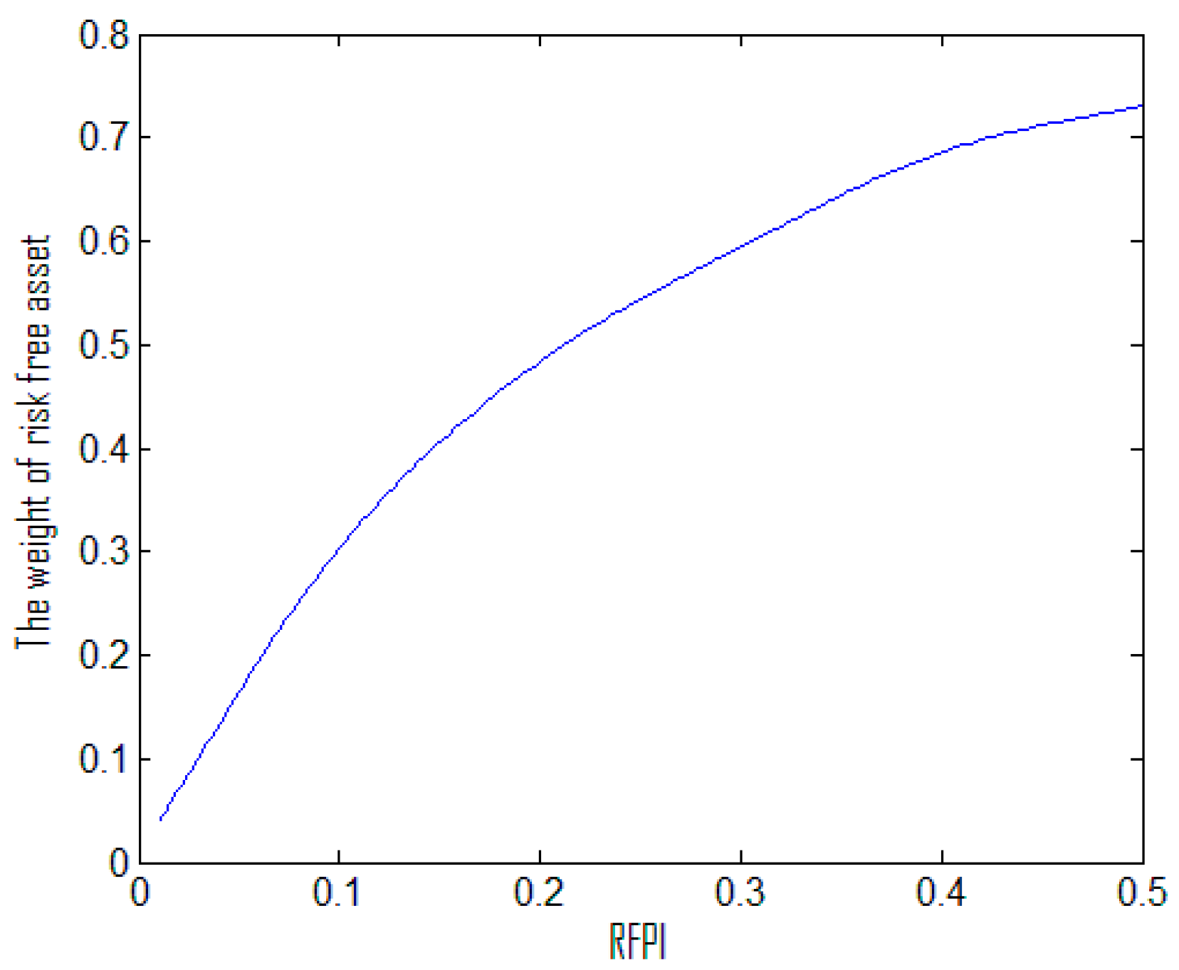
(i) The weight of the risk-free asset investment increases with the increase of the RFPI.

As portrayed in Figure 2, the weight of the risk-free asset investment is 31.49% when the risk-free protection index is 0.1. The weight of the risk-free asset investment also increases rapidly as the RFPI rises. When the RFPI rises to 50%, the weight of risk-free asset increases to 73.05%. This indicates that the investor should allocate more proportions to risk-free asset which can provide some protection for risk assets, and the protection proportion increases as the protection index increases.

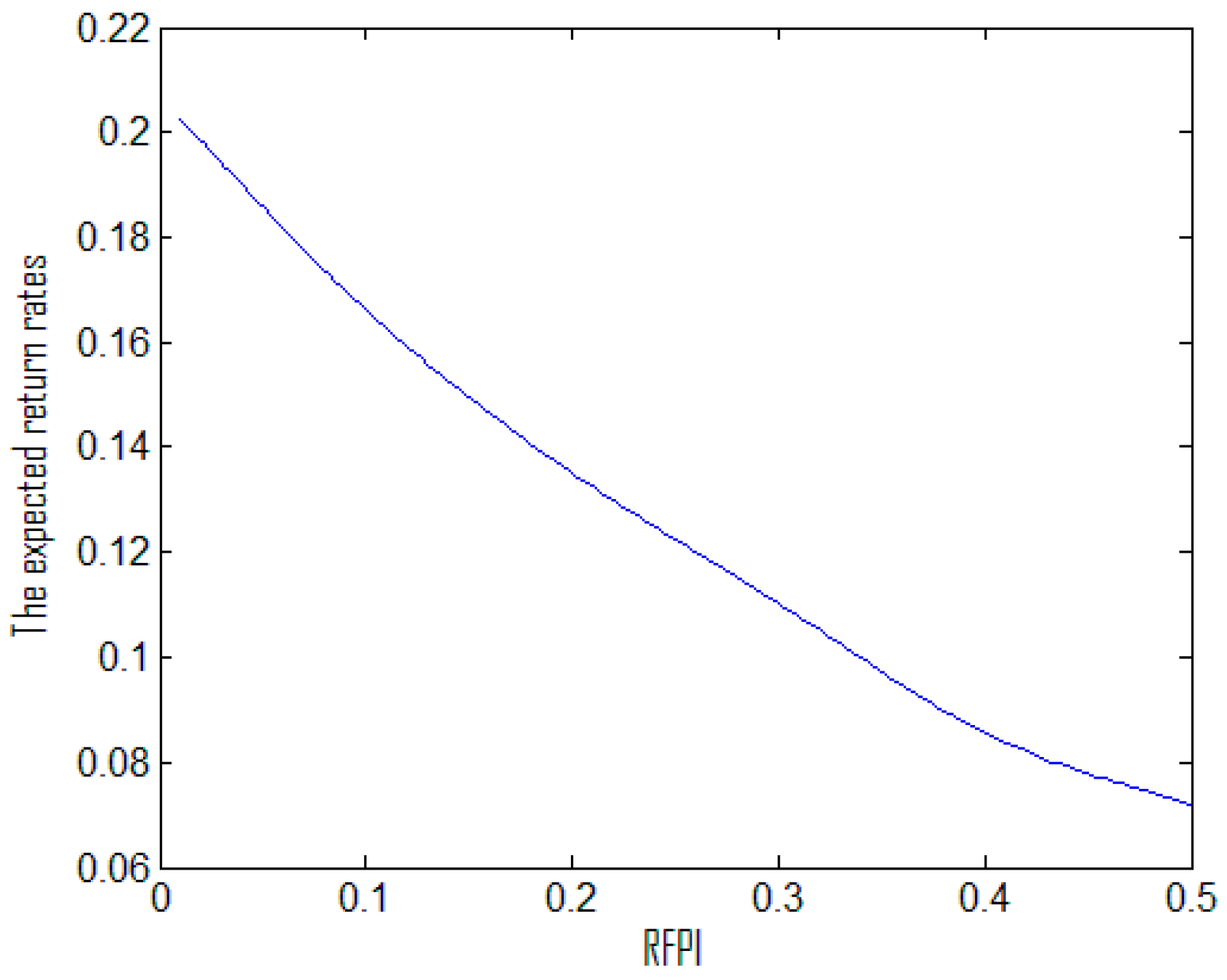
(ii) The expected return rate of the portfolio decreases with the increase of the RFPI.

As depicted in Figure 3, when the RFPI is 0.10, the expected return rate of the portfolio is 16.48%, which is far more than the risk free return rate 5%. When the RFPI rises to 50%, the portfolio expected return rate decreases to 7.19%. It implies that the portfolio return has a negative correlation with the RFPI and the investor should consider the potential risk when pursuing high returns.

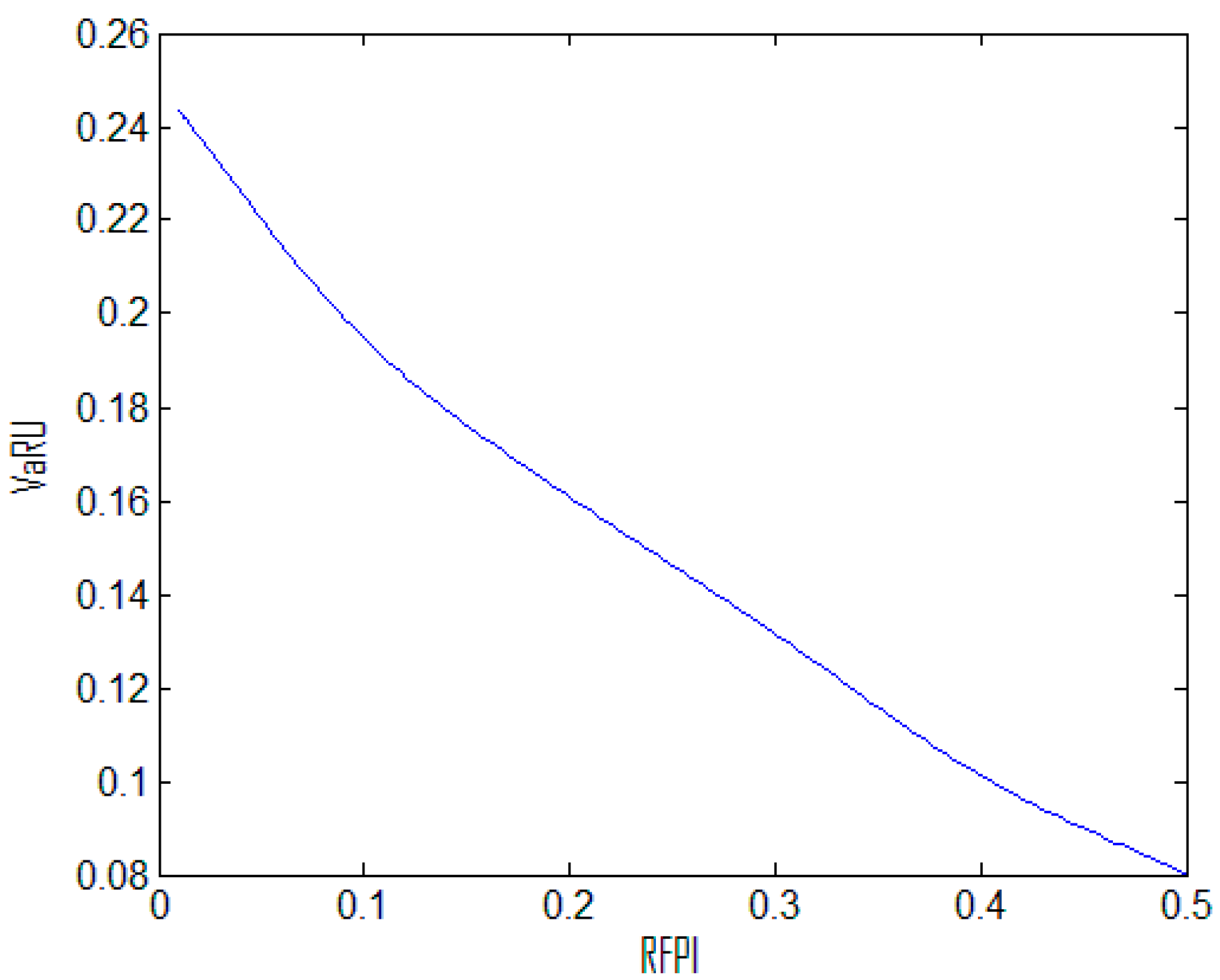
(iii) The VaRU of the portfolio decreases with the increase of the RFPI.

As described in Figure 4, the VaRU is up to 19.16% when the RFPI is 10%. As the RFPI increases to 50%, the VaRU decreases to 8.01%. We can see that the constraint of the VaRU becomes stricter when the RFPI is higher. Compared with the VaRU model, our model can search the optimal VaRU automatically under a certain RFPI value instead of subjective measurement, which is easy to see by combining Equations (12) with (13).

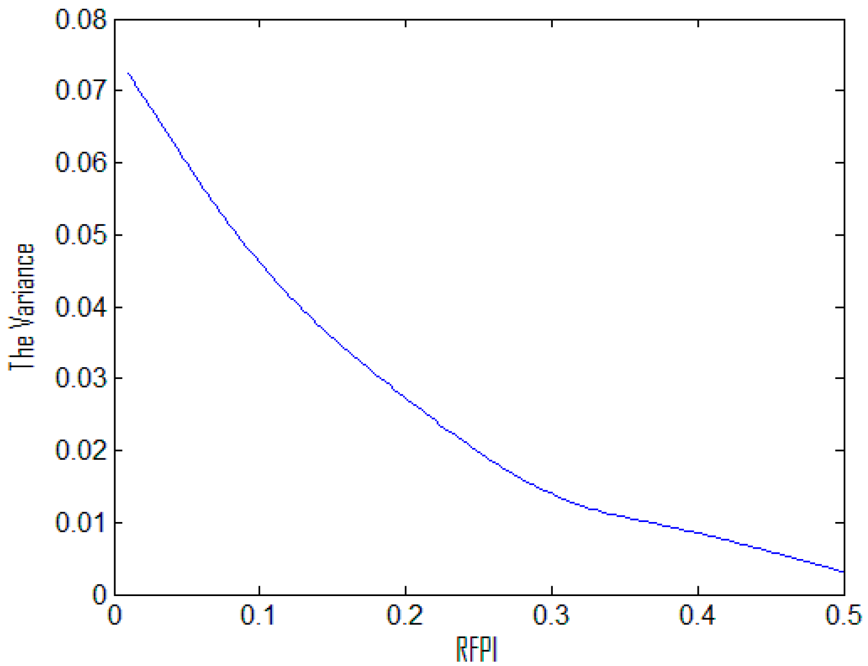
(iv) The variance of the portfolio decreases with the increase of the RFPI.

As shown in Figure 5, the portfolio variance also decreases as the RFPI increases. When the RFPI is 10%, the variance of the portfolio is 0.0445. The portfolio variance is only 0.0031 when the RFPI increases to 50%. This shows that RFPI can be used as a risk measure instead of variance, and the RFPI is more sensitive and stringent than variance. Therefore, it plays a very important role in setting the preset RFPI in portfolio selections. Especially, it suits the investors with high risk aversion or institution investors (e.g., pension fund investors).

5. Conclusions

This paper studied the protective screening effect of a risk-free security return on the portfolio selection expectations. We used uncertain variables to describe the security returns which are subject to experts’ evaluations and further proposed the risk-free protection index model under uncertainty framework. The RFPI was used to evaluate the protection made by risk-free asset when the risk assets happen to lose at a certain confidence level. Based on the RFPI, RIM for uncertain portfolio and MVEM for a diversified fuzzy portfolio, we put forward a risk-free protection index model with entropy constraint in uncertainty environment. Our study shows that the weight of the risk-free asset investment increases with the increase of the RFPI, while the expected return rate, the VaRU, and the variance of portfolio selection all decrease with the increase of the RFPI. Furthermore, the empirical results indicate that our proposed model is more meaningful and applicable in reality; it especially suits the investors with high risk aversion or institution investors.

In the paper, the author assumed that all return rates of $i$-th securities satisfied independent and normal uncertain distribution. However, not all return rates are independent because of the possible correlation effect among $i$-th securities in today’s highly related markets and the return rates of $i$-th securities don’t completely subject to normal uncertain distribution. Thus, we can take both the co-variance of a pair of assets in the model and abnormal uncertain distribution or other kinds of distributions into account in the future research. In addition, we can extend our portfolio selection problem to multi-objective portfolio problems and also add the crisp forms of the proposed model in the further study.