“Over-Learning” Phenomenon of Wavelet Neural Networks in Remote Sensing Image Classifications with Different Entropy Error Functions

Abstract

Artificial neural networks are widely applied for prediction, function simulation, and data classification. Among these applications, the wavelet neural network is widely used in image classification problems due to its advantages of high approximation capabilities, fault-tolerant capabilities, learning capacity, its ability to effectively overcome local minimization issues, and so on. The error function of a network is critical to determine the convergence, stability, and classification accuracy of a neural network. The selection of the error function directly determines the network’s performance. Different error functions will correspond with different minimum error values in training samples. With the decrease of network errors, the accuracy of the image classification is increased. However, if the image classification accuracy is difficult to improve upon, or is even decreased with the decreasing of the errors, then this indicates that the network has an “over-learning” phenomenon, which is closely related to the selection of the function errors. With regards to remote sensing data, it has not yet been reported whether there have been studies conducted regarding the “over-learning” phenomenon, as well as the relationship between the “over-learning” phenomenon and error functions. This study takes SAR, hyper-spectral, high-resolution, and multi-spectral images as data sources, in order to comprehensively and systematically analyze the possibility of an “over-learning” phenomenon in the remote sensing images from the aspects of image characteristics and neural network. Then, this study discusses the impact of three typical entropy error functions (NB, CE, and SH) on the “over-learning” phenomenon of a network. The experimental results show that the “over-learning” phenomenon may be caused only when there is a strong separability between the ground features, a low image complexity, a small image size, and a large number of hidden nodes. The SH entropy error function in that case will show a good “over-learning” resistance ability. However, for remote sensing image classification, the “over-learning” phenomenon will not be easily caused in most cases, due to the complexity of the image itself, and the diversity of the ground features. In that case, the NB and CE entropy error network mainly show a good stability. Therefore, a blind selection of a SH entropy error function with a high “over-learning” resistance ability from the wavelet neural network classification of the remote sensing image will only decrease the classification accuracy of the remote sensing image. It is therefore recommended to use an NB or CE entropy error function with a stable learning effect.

1. Introduction

Over the past several decades, artificial neural networks have become one of the hot study topics of remote sensing image classification [1,2,3,4], due to their good self-organization [5,6], self-learning [7,8], and self-adaptive abilities [9,10]. The back-propagation (BP) neural network is currently the most widely used artificial neural network [11,12,13,14]. Rumelhart proposed the BP algorithm as early as 1986 [15]. Although this algorithm is simple, and easy to master and realize, it still has deficiencies which include a slow convergence speed, a frequent non-convergence, a convergence to the local minimum, and so on. Considering the disadvantages of the BP neural network, Zhang et al. officially proposed the concept of a wavelet neural network in 1992 [16]. A wavelet neural network is constructed on the basis of the BP neural network, and in combination with the wavelet analysis theory. Comparing with the BP neural network, the wavelet neural network shows advantages in local information extraction and analysis, and also can overcome the defect of a slow convergence speed which characterizes the BP neural network. Currently, the most widely applied wavelet neural network is the BP wavelet neural network, which replaces the hidden-layer excitation function (sigmoid function) of the BP neural network with the wavelet function, and adopted the BP network ideology in order to perform the network learning and training. Currently, it is widely applied in remote sensing image classification [17,18,19].

An error function is the critical point in which to determine the convergence, stability, and classification accuracy of a neural network. The supervised learning algorithm is the core of the feed-forward neural network. This learning algorithm reversely changes the network’s weight and threshold value, in accordance with the function (error function) between the actual output and the anticipated output of a network, and minimizes the error value through repeated training in order to obtain the output and input relationship of a network [20]. The most commonly supervised learning method is the gradient descent method [15,21,22], and the most widely used error function in this method is the mean square error function. However, the curved surface of a mean square error function is the multi-dimensional hyper-surface with many flat zones and local minimum valleys. Therefore, it affects the convergence speed of a neural network, and can even be trapped in the local minimum point, which can easily cause a “false saturation” phenomenon [23]. The entropy error function proposed by Karayiannis in 1992 can be used to solve the “false saturation” phenomenon existing in the neural network training of a traditional mean square error function [24]. However, an “over-learning” phenomenon is often caused due to the too strong error signal of the NB entropy error function. In 1992, Ooyen et al. proposed the cross-entropy error function to improve the convergence of a neural network [25]. However, it also causes the “over-learning” phenomenon. Therefore, the scholar Oh SH modified the entropy error function in 1995, for the purpose of overcoming the “over-learning” phenomenon [26,27]. The above mentioned NB, CE, and SH entropy error functions are the most typical and widely used entropy error functions in neural networks.

Also, the above mentioned “over-learning” phenomenon usually occurs in circumstances which include simple characteristics and small data processing, such as handwriting recognition. However, for a remote sensing image classification with large calculation and processing, it is worthwhile to study whether an “over-learning” phenomenon exists in the neural network, and also whether it is necessary to use the SH entropy error function to resist the “over-learning” phenomenon. If the “over-learning” phenomenon does not exist or does not easily occur in the remote sensing image classification, then the blind use of the SH entropy error function resisting the “over-learning” phenomenon will sacrifice the accuracy of the classification. Therefore, it is necessary to systematically discuss the performances of the neural networks of the NB, CE, and SH entropy error functions in the remote sensing image classification, in order to answer the above questions and provide a basis for the selection of an entropy error function in a wavelet neural network.

In order to systematically study the performance of an entropy error function in remote sensing image classification, the remote sensing image types selected in this study cover the hyper-spectral image, multi-spectral image, high spatial resolution image, and Synthetic Aperture Radar (SAR), as well as other common remote sensing images. In this study, it is expected that the obtained conclusions will have a universality for the instruction of the selection of the entropy error function of the wavelet neural network in remote sensing image classifications. The characteristics of the remote sensing images, structure of neural networks, and training processes can possibly affect the performance of the “over-learning” phenomenon. Therefore, in order to comprehensively recognize the existence or non-existence and performance of an “over-learning” phenomenon, experimental studies of the above mentioned three influence factors were implemented in this study.

2. Method of Study

First, this paper introduces the wavelet neural network structure and entropy error function. Then, the mechanism and process of the “over-learning” phenomenon are explained, and finally the relationship between the three factors (characteristic of remote sensing image, structure of neural network, and training process) and the “over-learning” phenomenon are illustrated. This study also uses the experimental results to provide instructions for the selection of an entropy error function in a wavelet neural network.

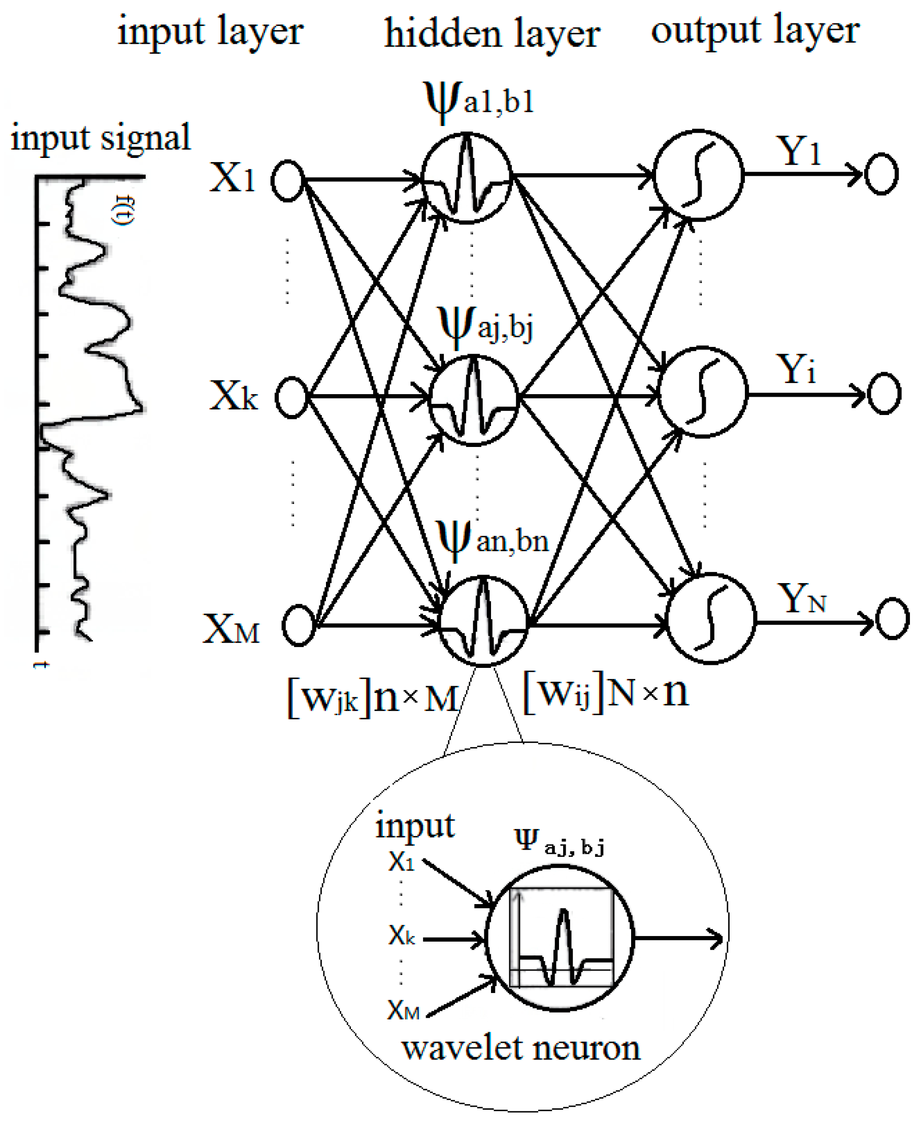
2.1. Structure and Training Process of the Wavelet Neural Network

The BP wavelet neural network applied in this study includes an input layer, hidden layer, and output layer. A corresponding weight value is used for connecting the input layer with the hidden layer, and the hidden layer with the output layer. The BP wavelet neural network structure of a single hidden layer is as shown in Figure 1. The training process of a wavelet neural network adopts the batch training method, with its flow process is as shown in Figure 2. It can be seen in this figure that P is the total number of samples, p indicates the p-th sample, and q denotes the number of trainings.

In which the excitation function of the hidden layer uses the Morlet wavelet function (see Equation (1)):

$$\psi \left(\mathrm{t}\right)=e^{(-\frac{t^2}{2})}\cos \left(1.75\mathrm{t}\right)$$

(1)

The wavelet neural network model is obtained by Equations (2)–(5):

$$ne{t}_j^p={\displaystyle \sum }_{k=1}^M{w}_{jk}{x}_k^p$$

(2)

$${\psi }_{a,b}\left(ne{t}_j^p\right)=\psi (\frac{ne{t}_j^p-b_j}{a_j})$$

(3)

$$y_i^p=f\left[{\displaystyle \sum }_{j=1}^n{w}_{ij}{\psi }_{a,b}\left(ne{t}_j^p\right)-{\beta }_i\right],i=1,2,\dots ,N$$

(4)

$$ne{t}_i^p={\displaystyle \sum }_{j=1}^n{w}_{ij}{\psi }_{a,b}\left(ne{t}_j^p\right)$$

(5)

The meaning of the parameters is as shown in

Table 1. Explanation of the parameter.

Parameter	Explanation
p (p = 1, 2, …, P)	number of input samples
k (k = 1, 2, …, M)	number of nodes in the input layer
j (j = 1, 2, …, n)	number of nodes in the hidden layer
i (i = 1, 2, …, N)	number of nodes in the output layer
${[w_{jk}]}_{n\times \mathrm{M}}$	weight matrix n × M from the input layer to the hidden layer, with $w_{jk}$ as the weight connecting node j of hidden layer with the node k of the input layer); (the initial value is a random value of [−1, 1])
${[w_{ij}]}_{N\times \mathrm{n}}$	weight matrix N × n from the hidden layer to the output layer, with $w_{ij}$ as the weight connecting the node i of the output layer and node j of the hidden layer; (the initial value is a random value of [−1, 1])
$x_k^p$	the kth input of the pth sample in the input layer
${\mathrm{net}}_j^p$	input of the jth node in the hidden layer of the pth sample
${\mathrm{net}}_i^p$	input of the ith node in the output layer of the pth sample
aj and bj	scaling parameter and translation parameter of the jth node of the hidden layer, respectively
${\psi }_{a,b}\left({\mathrm{net}}_j^p\right)$	output of the jth node of the hidden layer of the pth sample
${\beta }_i$	threshold value at the ith node of the output layer, (the initial value is a random value of [−1, 1])
$y_i^p$	the ith actual output in the output layer of the pth sample

.

The classification experiment process of the wavelet neural network is as follows:

(a)

The preprocessing of the original image is implemented, the features are extracted, and the expert interpretation chart is determined.

(b)

The region of interest is selected.

(c)

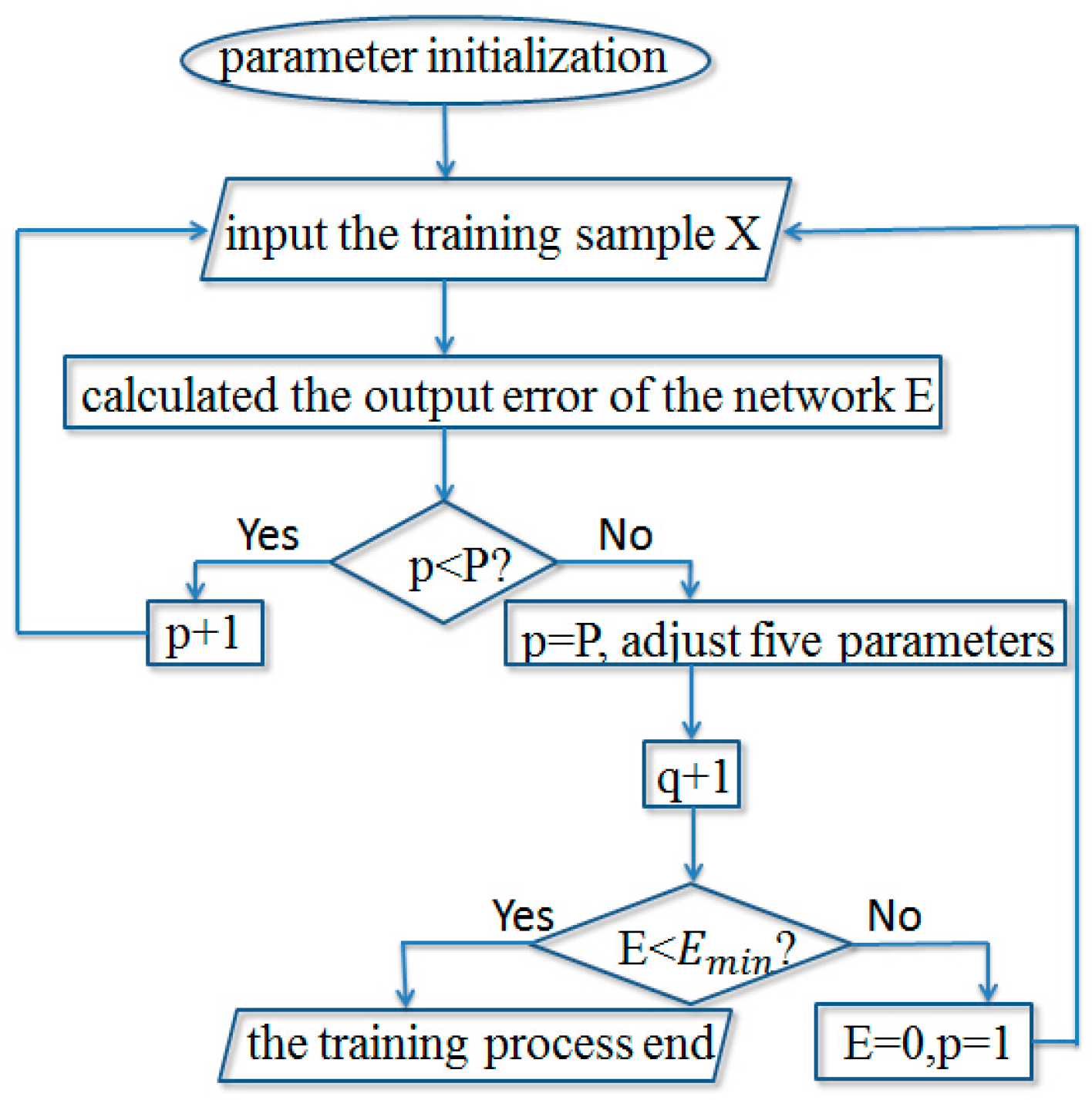
The wavelet neural network model is built, and the number of nodes in each layer is determined (numbers of the input layer nodes equal to numbers of features; numbers of the hidden layer nodes is determined by the testing; numbers of the output layer nodes equal to numbers of classified types), as shown in Figure 1.

(d)

The characteristic value of the pixels in the region of interest is used as the input, in order to conduct the training of the wavelet neural network. Setting the number of times of iterations is 100. Setting the output minimum error E_min of the neural is 1 × 10⁻⁵. If the output error E < E_min, then end the training. If the E > E_min, then repeat training the network.

(e)

The classification result is simulated in order to obtain the classification results of the diagram, and make an accuracy assessment of classification.

(f)

The number of nodes of the hidden layer and the number of iterations are adjusted. Trainings are conducted and classification results of the networks with different entropy error function are compared.

2.2. Entropy Error Function

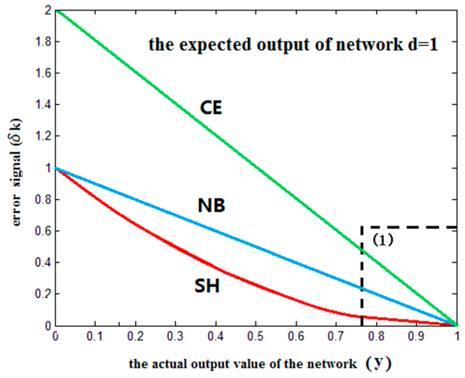
2.2.1. NB Entropy Error Function

The NB entropy error function of the wavelet neural network adopted the entropy error function proposed by Karayiannis NB in 1992, as shown in Formula (6). The wavelet neural network of the NB entropy error function requires $0<y_i^p<1$ Therefore in this study, the log-sigmoid function is selected (as shown in Formula (7)) as the nerve cell excitation function of the output layer:

$$\mathrm{E}=-{\sum }_{p=1}^P{\sum }_{i=1}^N\left[d_i^p\ln y_i^p+\left(1-d_i^p\right)\ln \left(1-y_i^p\right)\right]$$

(6)

In which E is the network error; $d_i^p$ is the ith expected output of the pth sample in the output layer; and $y_i^p$ is the ith actual output of the pth sample in the output layer:

$$f\left(t\right)=\frac{1}{1+e^{-t}}$$

(7)

2.2.2. CE Entropy Error Function

The CE entropy error function of the wavelet neural network adopted the cross-entropy error function proposed by Ooyen et al. in 1992, as shown in Equation (8). The wavelet neural network of the cross-entropy error function required $-1<y_i^p<1$. Therefore, the tan-sigmoid function is selected (as shown in Formula (10)) as the nerve cell excitation function of the output layer:

$$\mathrm{E}=-{\displaystyle \sum }_{p=1}^P{\displaystyle \sum }_{i=1}^N\left[(1+d_i^p\right)\ln \left(1+y_i^p\right)+\left(1-d_i^p\right)\ln \left(1-y_i^p\right)]$$

(8)

2.2.3. SH Entropy Error Function

The SH entropy error function of the wavelet neural network adopted the entropy error function proposed by Oh in 1995, as shown in Equation (9). The wavelet neural network of the SH entropy error function required $-1<y_i^p<1$. Therefore, the tan-sigmoid function is selected (as shown in Formula (10)) as the nerve cell excitation function of the output layer of the output layer:

$$\mathrm{E}=-{\displaystyle \sum }_{p=1}^P{\displaystyle \sum }_{i=1}^N{d}_i^p[-y_i^p+\frac{1+{d_i^p}^2}{2}\ln \frac{1+y_i^p}{1-y_i^p}+d_i^p\ln \left(1-y_i^p\right)\left(1+y_i^p\right)]$$

(9)

$$f\left(t\right)=\frac{2}{1+e^{-2t}}-1$$

(10)

The gradient information could be deduced by using the network model, and the entropy error formula (as shown in

Table 2. Gradient of error function.

Gradient	NB Error Function	CE Error Function	SH Error Function
$\frac{\partial E}{\partial w_{jk}}$	${\displaystyle {\displaystyle \sum }_{p=1}^P}{\displaystyle {\displaystyle \sum }_{i=1}^N}\left(y_i^p-d_i^p\right)w_{ij}{\psi }^{\prime }\left(ne{t}_j^p\right)x_k^p/a_j$	${\displaystyle {\displaystyle \sum }_{p=1}^P}{\displaystyle {\displaystyle \sum }_{i=1}^N}2\left(y_i^p-d_i^p\right)w_{ij}{\psi }^{\prime }\left(ne{t}_j^p\right)x_k^p/a_j$	$-{\displaystyle {\displaystyle \sum }_{p=1}^P}{\displaystyle {\displaystyle \sum }_{i=1}^N}{d}_i^p\frac{{\mathrm{w}}_{\mathrm{ij}}{{\psi }_{a,b}}^{\prime }\left(ne{t}_j^p\right)x_k^p}{a_j}·{\left(y_i^p-d_i^p\right)}^2$
$\frac{\partial E}{\partial w_{ij}}$	${\displaystyle {\displaystyle \sum }_{p=1}^P}\left(y_i^p-d_i^p\right){\psi }_{a,b}\left(ne{t}_j^p\right)$	${\displaystyle {\displaystyle \sum }_{p=1}^P}2\left(y_i^p-d_i^p\right){\psi }_{a,b}\left(ne{t}_j^p\right)$	$-{\displaystyle {\displaystyle \sum }_{p=1}^P}{\displaystyle {\displaystyle \sum }_{i=1}^N}{d}_i^p{\psi }_{a,b}\left(ne{t}_j^p\right)·{\left(y_i^p-d_i^p\right)}^2$
$\frac{\partial E}{\partial a_j}$	${\displaystyle {\displaystyle \sum }_{p=1}^P}{\displaystyle {\displaystyle \sum }_{i=1}^N}\left(d_i^p-y_i^p\right)w_{ij}{\psi }^{\prime }\left(ne{t}_j^p\right)(ne{t}_j^p-b_j)/a_j^2$	${\displaystyle {\displaystyle \sum }_{p=1}^P}{\displaystyle {\displaystyle \sum }_{i=1}^N}2\left(d_i^p-y_i^p\right)w_{ij}{\psi }^{\prime }\left(ne{t}_j^p\right)(ne{t}_j^p-b_j)/a_j^2$	$-{\displaystyle {\displaystyle \sum }_{p=1}^P}{\displaystyle {\displaystyle \sum }_{i=1}^N}\frac{d_i^p{\mathrm{w}}_{\mathrm{ij}}{{\psi }_{a,b}}^{\prime }\left(ne{t}_j^p\right)\left(b_j-w_{jk}{x}_k^p\right)}{{a_j}^2}·{(y_i^p-d_i^p)}^2$
$\frac{\partial E}{\partial b_j}$	${\displaystyle {\displaystyle \sum }_{p=1}^P}{\displaystyle {\displaystyle \sum }_{i=1}^N}\left(d_i^p-y_i^p\right)w_{ij}{\psi }^{\prime }\left(ne{t}_j^p\right)/a_j$	${\displaystyle {\displaystyle \sum }_{p=1}^P}{\displaystyle {\displaystyle \sum }_{i=1}^N}2\left(d_i^p-y_i^p\right)w_{ij}{\psi }^{\prime }\left(ne{t}_j^p\right)/a_j$	$-{\displaystyle {\displaystyle \sum }_{p=1}^P}{\displaystyle {\displaystyle \sum }_{i=1}^N}{d}_i^p{\mathrm{w}}_{\mathrm{ij}}{{\psi }_{a,b}}^{\prime }\left(ne{t}_j^p\right)(\frac{-1}{a_j})·{(y_i^p-d_i^p)}^2$
$\frac{\partial E}{\partial {\beta }_i}$	${\displaystyle {\displaystyle \sum }_{p=1}^P}\left(d_i^p-y_i^p\right)$	${\displaystyle {\displaystyle \sum }_{p=1}^P}2\left(d_i^p-y_i^p\right)$	$-{\displaystyle {\displaystyle \sum }_{p=1}^P}{\displaystyle {\displaystyle \sum }_{i=1}^N}(-d_i^p)·{(y_i^p-d_i^p)}^2$

Note: The meanings of the parameters in the formula correspond with the above content.

).

2.3. “Over-Learning” Phenomenon and Method of Study

2.3.1. “Over-Learning” Phenomenon

The “over-learning” of the network is relative to the normal learning. When the actual output is close to the expected output during the network training process, then the network has a weak “error signal”. Or when there is a large gap between the actual output and expected output, then the network has strong “error signal”. Then the network is referred to as the “normal learning”. In contrast, when the actual output is close to the expected output, and the network had a strong error signal, then the network continues to learn, and two possibilities exist. The first possibility is that when the network weight value is not close to the optimum value, the network weight value causes the network simulation degree to increase in the case of continuous learning. The second possibility is that when the network weight value has already been close to the optimum network weight value, then the network weight value is disturbed in the case of continuous learning, and the network simulation degree decreases. This is referred to as the “over-learning”.

The network error signal ${\delta }_i$ can be calculated using the error formula and the network model, as shown in Equation (11), in which, η is the network learning rate:

$${\delta }_i=-\frac{\partial E}{\partial ne{t}_i^p}=-\eta \frac{\partial E}{\partial y_i}·\frac{\partial y_i}{\partial ne{t}_i^p}$$

(11)

The error signal of the mean square error function, NB error function, CE error function and SH error function, can be calculated using Equation (11) (see Equations (12)–(15)):

$$\text{Mean square}: {\delta }_i=\left(d_i-y_i\right)y_i\left(1-y_i\right)$$

(12)

$$\text{NB}: {\delta }_i=d_i-y_i$$

(13)

$$\text{CE}: {\delta }_i=2\left(d_i-y_i\right)$$

(14)

$$\text{SH}: {\delta }_i=d_i{\left(d_i-y_i\right)}^2$$

(15)

Figure 3 shows the corresponding signal values of the three error entropy functions (NB, CE, and SH) with the change of the actual output y from 0 to 1, when the expected output of the network d = 1. In this study, the fiducial mark (1) area is focused on, and it is discovered that the “over-learning” more easily occurs with the NB and CE. Meanwhile, with the SH the “over-learning” does not easily occur, indicating that the SH has an “over-learning” resistance ability. This is due to the fact that the SH gives a weak “error signal” when the actual output is close to the expected output, while the entropy functions NB and CE give strong error signals, Therefore the network can continue to learn. It is therefore determined that in the neural network of the entropy error functions NB and CE, the “over-learning” phenomenon more easily occurs (see Figure 4 for its performance).

In this study, during the learning process of network parameters, it cannot be guaranteed that the network has a good prediction and generalization capacity to the unknown samples when the error function reaches the minimum value [28]. The “over-learning” phenomenon shows that the image classification accuracy is difficult to improve upon, or that the event decreases with the decreasing of the error, when the network training error drops to a certain degree (as shown in Figure 4).

2.3.2. Study Method for the “Over-Learning” Phenomenon

In order to study whether there is an “over-learning” phenomenon in the wavelet neural network (WNN) remote sensing image classification, as well as the existing conditions and performance of the “over-learning” phenomenon, this study investigates from the following two aspects: on the one hand, starting from the input information of the neural network, the relationship between the image characteristics and the “over-learning” phenomenon are discussed; on the other hand, starting from the self-structure of the neural network, the relationship between the neural networks with different numbers of nodes in the hidden layer (reflecting the differences in the neural network structure), and the number of iterations of the neural network (reflecting the training process of the neural network), along with the “over-learning” phenomenon are analyzed. A comparison is made between the classification accuracy obtained from the experimental study, and the minimum error value. When the corresponding minimum error value of the training sample is low and the image classification accuracy is low, this shows that an “over-learning” phenomenon has occurred in the neural networks.

Remote Sensing Image Characteristics and the “Over-Learning” Phenomenon

In order to study the relationship between the image characteristics and the “over-learning” phenomenon, it is necessary to establish a method of describing the image characteristics. For this purpose, the factors of the image’s complexity, as well as the image size are considered. The phenomenon of the “same object with different spectrums” commonly exists in remote sensing images, and its differences of degree will increase the complexity of the classification, as well as affect the automatic classification accuracy of the remote sensing images [29]. In order to quantitatively describe the characteristics of the phenomenon of the “same object with different spectrums”, the index SP for the phenomenon of “same object with different spectrums” is proposed. In addition, the information entropy of the images represents the complexity of the images. The class numbers of the remote sensing image classifications, image pixels (image size), and number of wave bands of the input images, are related to the input of the neural network [30,31].

The image complexity index AI reflects the degree of complexity of the images in this paper. The larger the AI value indicates more information is in the images or image is more complex. Computation formula of AI is defined as follows:

$$\mathrm{AI}=\mathrm{KN}+\mathrm{SP}+\mathrm{H}\times 0.1+\mathrm{M}+\mathrm{P}\times 0.0001$$

(16)

In which AI is the complexity index of the image; KN is the number of categories contained in the image; SP is the index describing the “same object with different spectrums” of the image; H is the information entropy describing the image information quantity; M is the number of wave bands of effective characteristics of the image; and P is the total number of pixels of the image. The index SP of the “same object with different spectrums” refers to the difference of the spectrum characteristic values of the same type of ground feature, and reflects the degree of the “same object with different spectrums” of the image. SP(t) is the spectral difference value of the tth type of ground feature; $x_i$ is the characteristic value of the ith pixel point; and N is the total number of pixels of the tth type of ground feature of the image as follows:

$$\overline{x}=\frac{{\sum }_{i=1}^N{x}_i}{N}$$

(17)

$$\mathrm{SP}\left(t\right)=\frac{\left(\frac{{\sum }_{i=1}^{N-1}{\left(x_i-x_{i+1}\right)}^2}{N-1}\right)+(\frac{{\sum }_{i=1}^N{\left(x_i-\overline{x}\right)}^2}{N})}{2}$$

(18)

Shannon proposed the definition of information and information entropy in 1948 [32]. Within the field of image processing, the information entropy indicates a type of characteristic parameter used for the measurement of the gray-scale distribution randomness in the gray level co-occurrence matrix, and reflects the size of the average information in an image. The larger the information entropy, the larger the information size of an image, and the higher the degree of complexity.

Number of Hidden Nodes and “Over-Learning” Phenomenon in the Neural Network

The number of the hidden layer neural nodes of the neural network is one of the factors which determine the neural network structure. In order to fully investigate the impact of the three types of entropy error functions on the wavelet neural networks with different structures, a classification experiment with a different number of hidden layer nodes is conducted, and the relationship with the “over-learning” phenomenon is discussed. Also, the number of hidden layer nodes is arranged from small to large, in order to make a classification of the different images, provided that the other parameters of the network remained unchanged. With the increase in the number of hidden layer nodes, the network scale also gradually increases. It is then observed whether the network approximation ability displays a surplus and “over-learning” phenomenon in the experimental results.

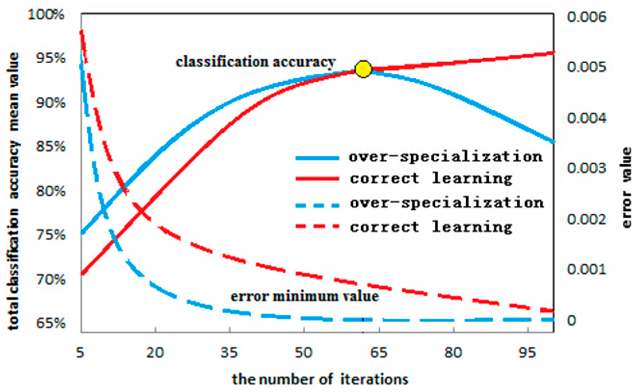
Investigation of “Over-Learning” Phenomenon through the Training Process of the Neural Network

The focus of this study is to investigate the “over-learning” phenomenon through the training process of the neural network, which will be helpful for understanding the “over-learning” phenomenon. In this study’s designed experiment, only the number of iterations of the neural network is changed, and the other parameters are not changed. Then, the change process of the training error value, as well as the classification accuracy of the three different entropy error function networks (NB, CE, and SH) with the increase of the number of the iterations of the neural network are observed, for the purpose of judging whether the network had an “over-learning” phenomenon, and also to judge its performance. For one image with the same interest of region and initial weight condition, the number of hidden layer nodes is set, the number of iterations is increased from small to large, and then the classification of these three types of entropy error function networks is performed three times, in order to obtain overall accuracy mean value of the classification and the minimum error value curve.

3. Experiment and Analysis

3.1. Experiment Images

3.1.1. Data of Experiment 1

Remote sensing image of sea-ice (as shown in Figure 5). This data contain seven characteristic images extracted from the SAR image of the sea-ice. They are: the volume scattering image of the LEE filtering of the C waveband; the volume scattering image of the LEE filtering of the L waveband; the entropy image of the LEE filtering of the L waveband; the anisotropy image of the LEE filtering of the C wave band; and the principal component analysis images of the 1st, 2nd, and 3rd principal component wavebands.

3.1.2. Data of Experiment 2

The Indian pines hyper-spectral data (as shown in Figure 6) is an image obtained from AVIRIS on 12 June 1992; with a wave length scope of 0.4 to 2.5 μm, a spectral resolution of 10 nm, and a spatial resolution of 17 m; there are a total of 220 wave bands. 20th, 23rd, 29th, 32nd, 33rd, 35th, 54th, 56th, 87th and 116th wave bands (10 in total) are selected as the classification experiment input in accordance with [33]. The ground features are divided into nine classes, in accordance with the actual ground circumstances.

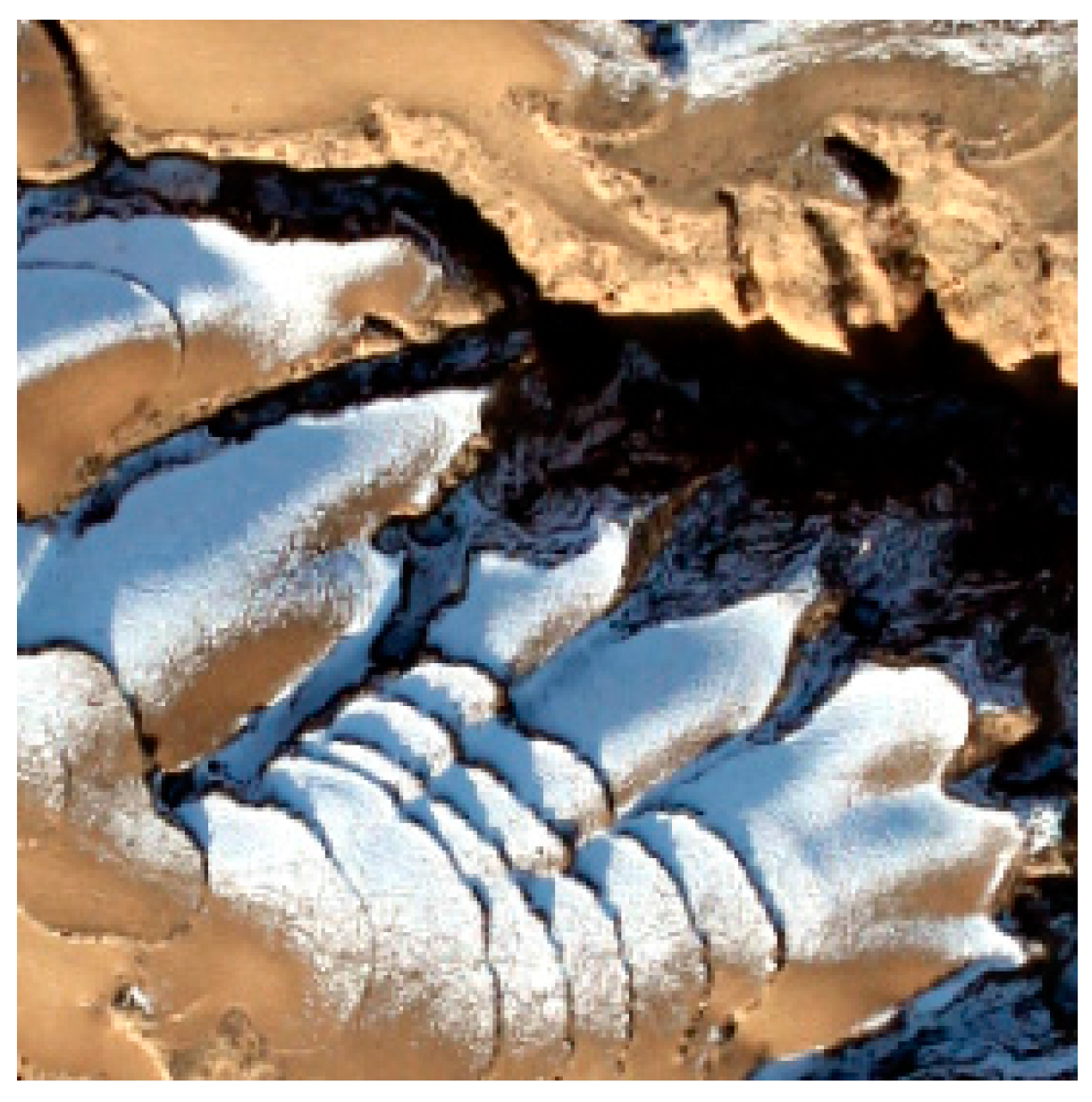
3.1.3. Data of Experiment 3

A high-resolution image of the snow mountain (as shown in Figure 7), obtained by using a Canon 5D Mark II digital camera with a spatial resolution of 0.2 m. This study uses three spectral characteristic images, and 6 R-channel 3 × 3 window texture characteristic images, which are the mean value, mean square, homogeneity, contrast ratio, non-similarity, and entropy, respectively.

3.1.4. Data of Experiment 4

The TM data in Nanjing District (as shown in Figure 8), obtained on 5 July 1988. The with spatial resolution of all of wave bands is 30 m, with the exception of the thermal infrared band, which is 120 m, and there are a total of seven wave bands.

3.1.5. Data of Experiment 5

The high-resolution image of houses (as shown in Figure 9), obtained using a Canon 5D Mark II digital camera carried by an unmanned aerial vehicle; spatial resolution is 5 cm.

3.1.6. Data of Experiment 6

The hyper-spectral data of Heihe (as shown in Figure 10) obtained from the comprehensive remote sensing observation joint experiment of the ecological-hydrological process in the Heihe River Basin [34], which is an airborne hyper-spectral data of a flight lasting 12 h 26′ 42″ on 29 June 2012. The sensor is a Compact Airborne Spectrographic Imager CASI produced by ITRES Co. (Calgary, AB, Canada), with a wavelength of 350 to 1050 nm, 48 spectral channels (7.2 nm, FWHM), and a spatial resolution of 1 m.

3.2. Result Analysis of “Over-Learning” Phenomenon

3.2.1. Investigation of “Over-Learning” Phenomenon through the Training Process of Neural Network

The focus of this study is to investigate the overall training process and simulation results of a neural network, which will be helpful for understanding the “over-learning” phenomenon. Through the analysis of the “over-learning” mechanism of a network (Figure 3 and Figure 4), it is determined that the SH entropy error function network has an “over-learning” resistance ability, while the NB and CE entropy error function networks do not have such abilities. With the increase in the number of iterations, the classification accuracy is compared with the minimum error value. When the corresponding minimum error value of a training sample drops to the lowest level, and the image classification accuracy is decreased, these results indicates that the neural networks exhibited an “over-learning” phenomenon. In the same experiment, if the classification accuracy of the SH entropy function network is higher than that of the NB or CE, but its minimum error value is larger than that of the NB and CE, then it is believed that the NB and CE networks exhibits an “over-learning” phenomenon, otherwise the networks never undergo the “over-learning” phenomenon. It can be determined from Figure 11, Figure 12 and Figure 13 that:

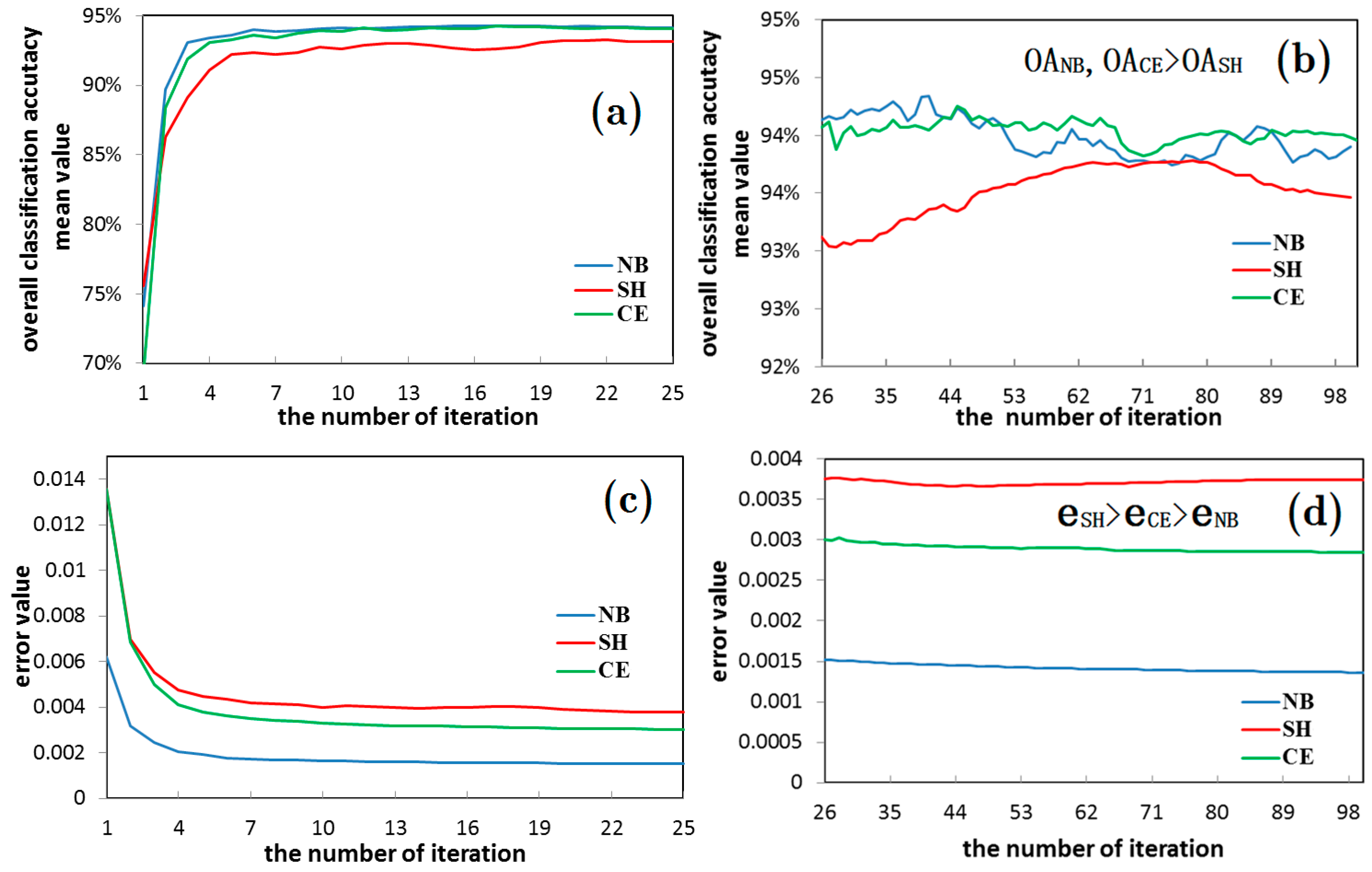
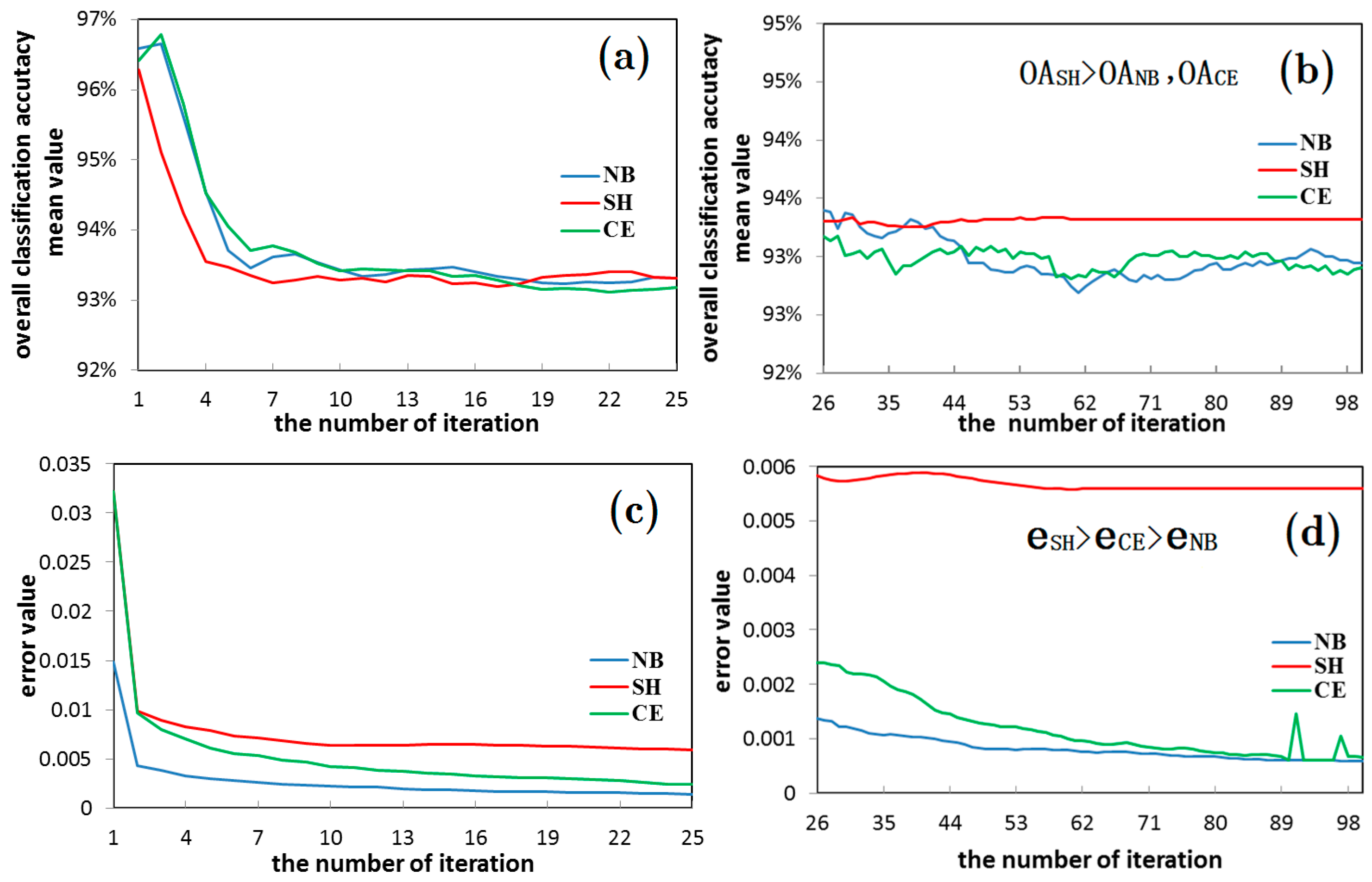
• A network will exhibit an over-learning phenomenon only for a very small size of images with a very low complexity degree. The lager the image size, the larger the AI index of an image, the more complex an image. In the case of that, the “over-learning” phenomenon will not be frequent. During the experiment, the “over-learning” phenomenon is obvious only in the 50 × 50 high-resolution image of houses, and hyper-spectral image of Heihe, which has the smallest AI index. At that time, the minimum error value of the SH entropy error function neural network is larger than that of NB and CE. However, the classification accuracy of the SH entropy error network is higher than that of the NB and CE. Therefore, the SH entropy error network shows a good “over-learning” resistance ability, while the NB and SH entropy error function networks exhibits the “over-learning” phenomenon.
• In most experiments (SAR, multi-spectral, and hyper-spectral image), the classification accuracy of the SH entropy error is lower than that of the NB and CE, and the classification accuracy of the SH entropy error will be higher than NB and CE only when the image complexity degree is very low. These results in fact show that the wavelet neural network for the remote sensing image will not easily cause an “over-learning” phenomenon. Also, the NB and CE networks will exhibit an “over-learning” phenomenon only when the image is small, such as merely containing 50 × 50 pixels (however, this is rare).

3.2.2. Remote Sensing Image Characteristics and “Over-Learning” Phenomenon

In order to study the “over-learning” phenomenon in the WNN remote sensing image classification, four rectangular subsets are created from the high-resolution images of houses, and the hyper-spectral images of Heihe (as shown in Figure 14 and Figure 15). The calculation results of their AI index values shows the law of changing from small to large. These four rectangular zones represent the images whose “same object with different spectra” phenomenon changed from less to more; the complexity degree of ground features changed from low to high; and the separability changed from strong to weak, respectively. The number of iterations is set at 100 with a different number of hidden layer nodes, and the four rectangular zones are classified 30 times, using three types of entropy error function neural networks, in order to obtain the image characteristic AI value of the four rectangular zones (as shown in Figure 14 and Figure 15), as well as the WNN classification result of the four rectangular zones (as shown in Figure 16 and Figure 17):

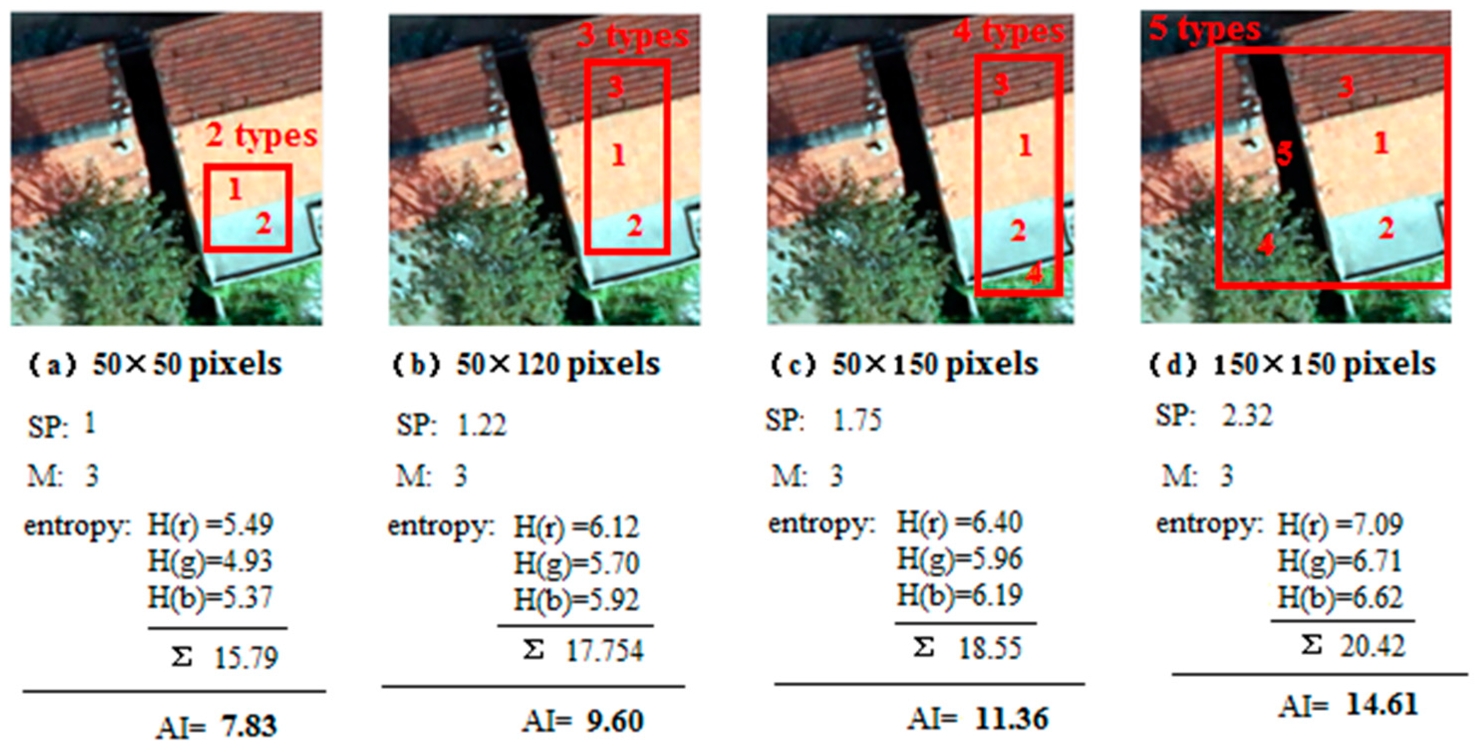
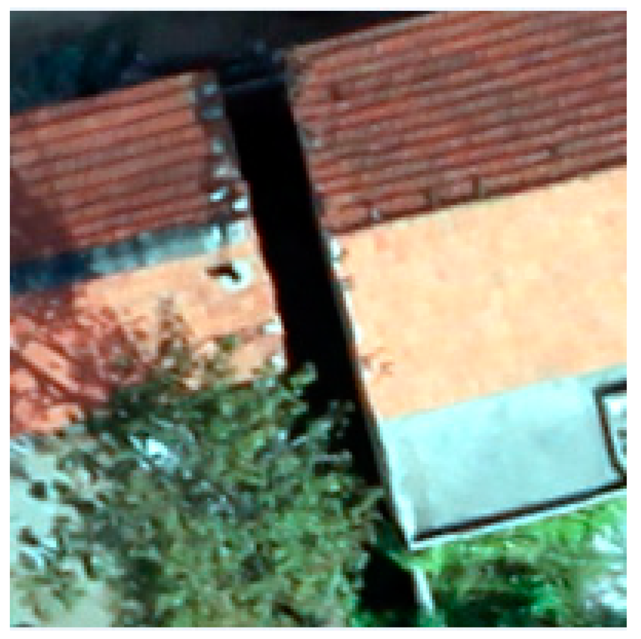
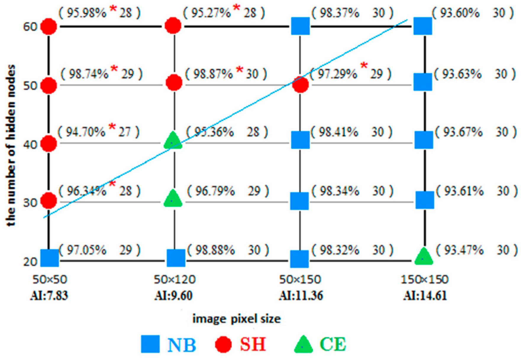
• It is found in the classification experiment of high-resolution image of houses (as shown in the Figure 14 and Figure 16) that the SH entropy function network has a higher overall classification accuracy than the NB and CE under the small pixel image (50 × 50 pixels), or when the image characteristic is simple. This is more obvious when the number of hidden layer nodes is increased. For example, in the 50 × 50 pixels image classification (AI index was 7.82), the classification accuracy of the SH entropy error network with four hidden layer nodes (30, 40, 50, and 60) is higher than the NB or CE. This indicates that the NB and CE entropy error function network has a surplus learning ability, and experienced an “over-learning” phenomenon, while the SH network has a moderate learning ability, and an “over-learning” resistance ability. Therefore, the SH error function is the recommended selection.
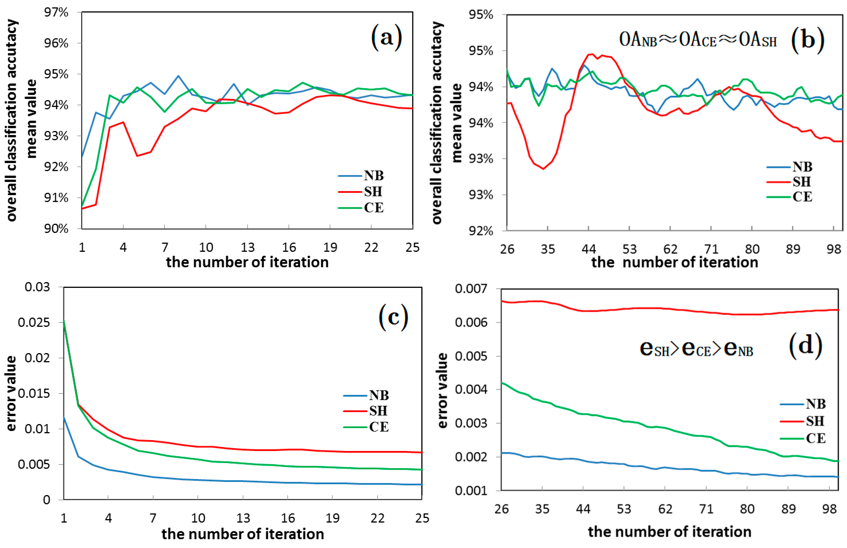
• In the large-pixel images, the classification accuracy of the NB and CE entropy error function network is found to be higher than the SH, with the increase of the complexity degree of the ground features. For example, in the 150 × 150 pixel image classification (AI index was 14.61, and the complexity degree of image obviously rises compared with the 50 × 50 pixel), for the five hidden layer nodes, the classification accuracy of the NB and CE entropy error function network is higher than the SH. These results indicate that the network learning ability is not in surplus and an “over-learning” phenomenon does not exist. Therefore in this study, the NB or CE entropy error functions are commended to be selected in order to guarantee the classification accuracy of the network.
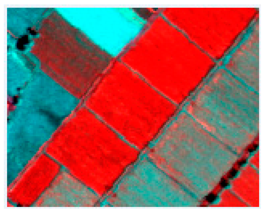
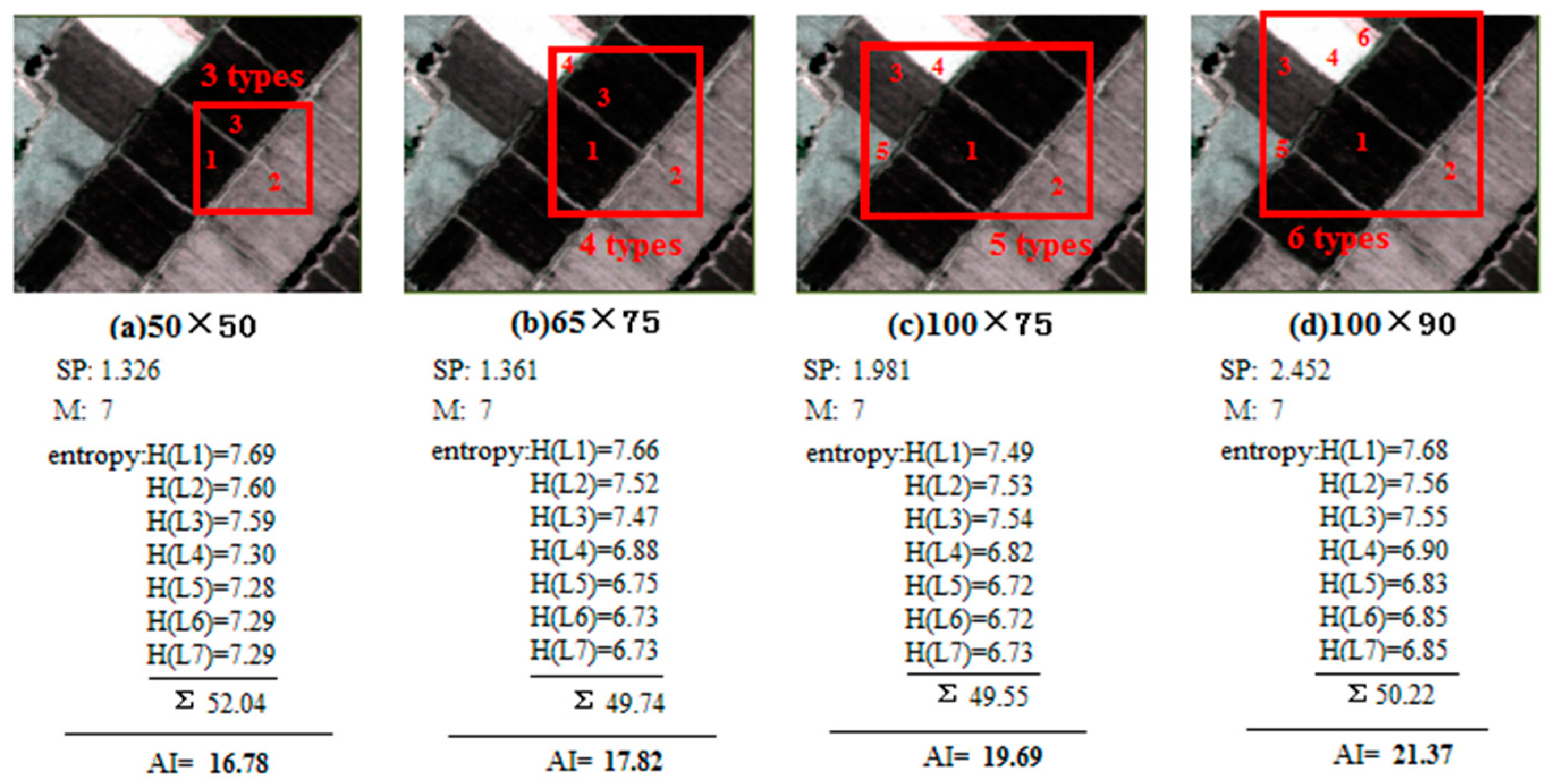
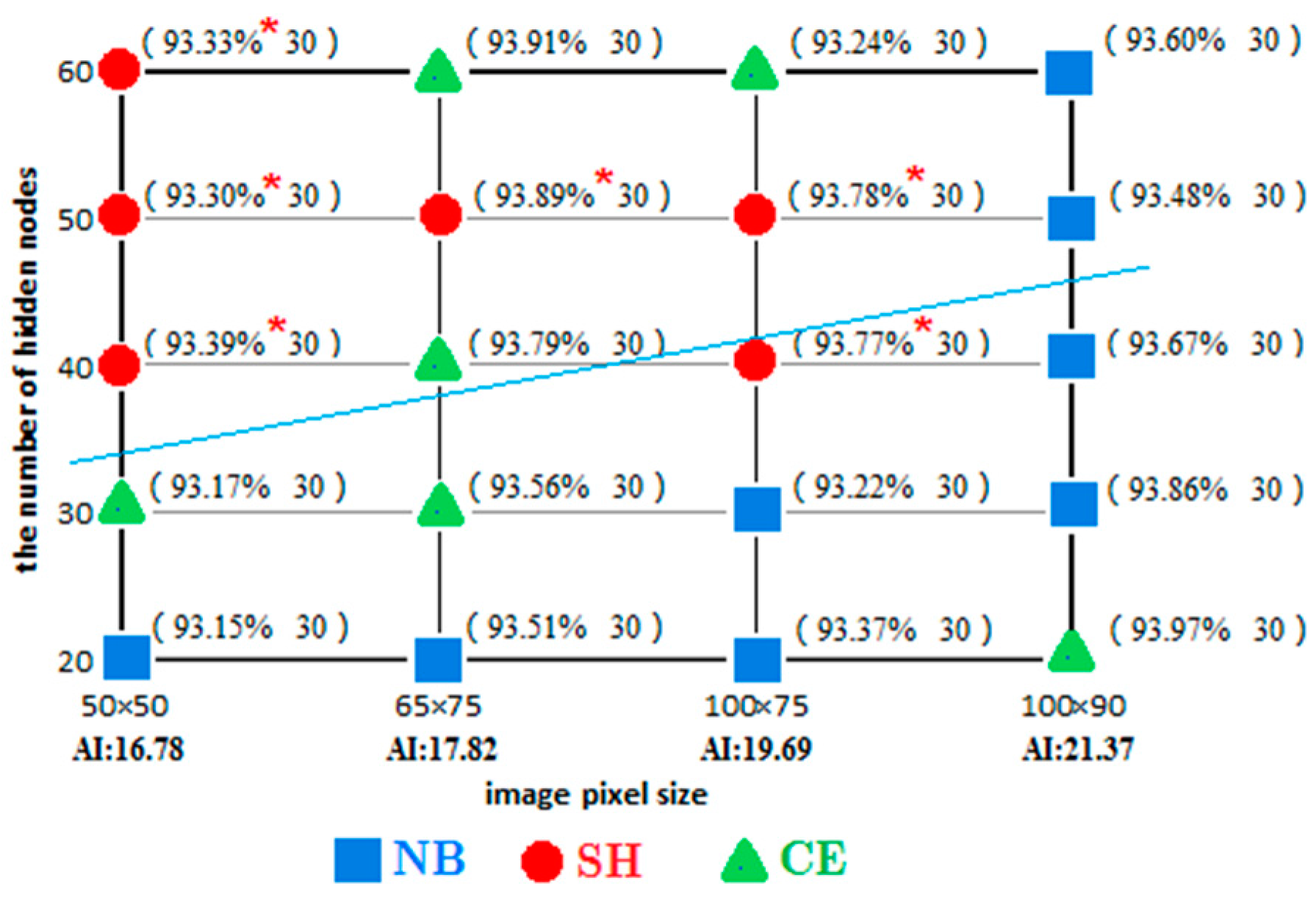
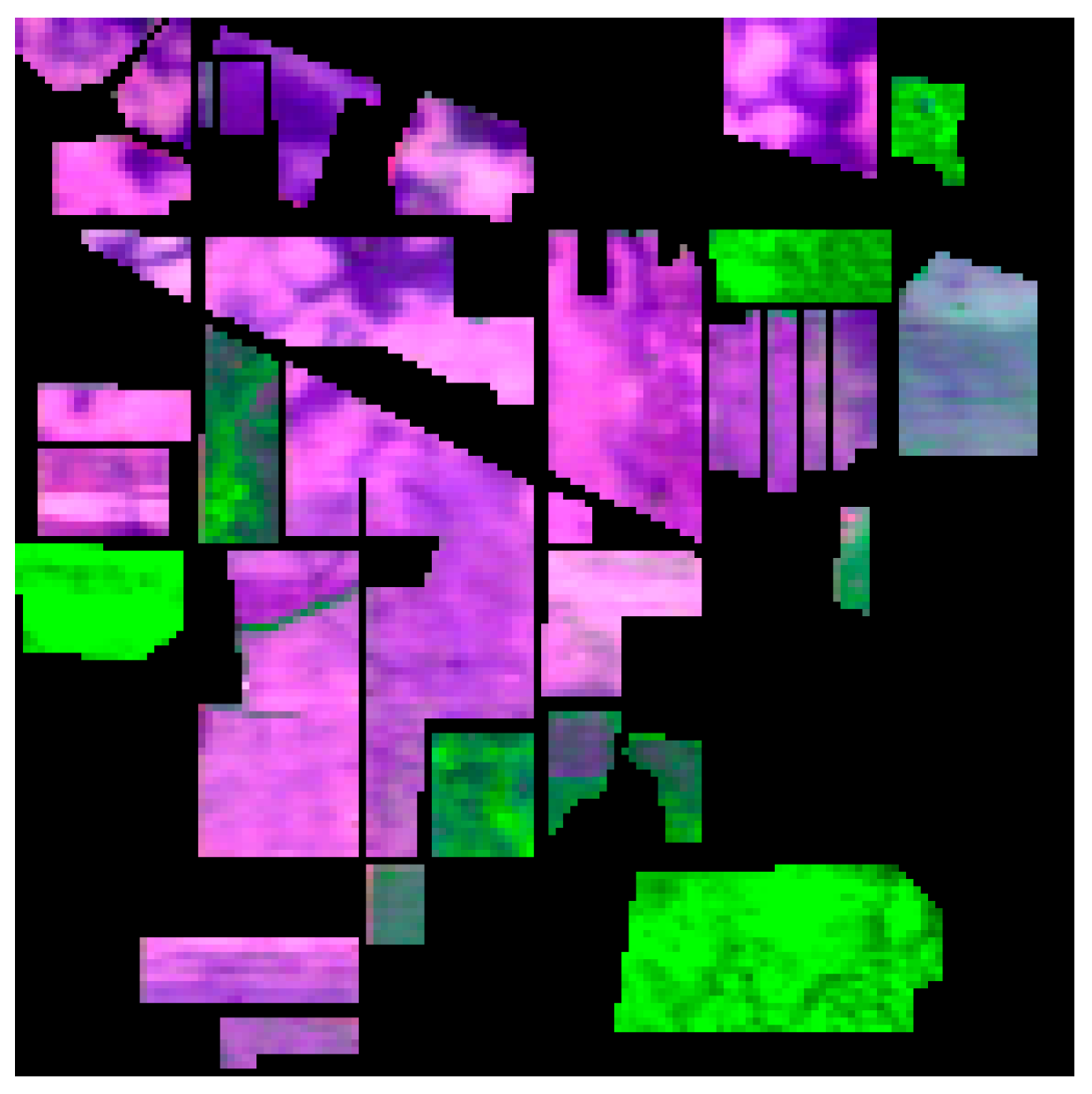
• There was also a similar law in the hyper-spectral image of the Heihe River. For example, the network easily has an “over-learning” phenomenon when the image complexity degree is low with the small image condition. Meanwhile, with the large image condition, the network does not easily have an “over-learning” phenomenon when the image complexity degree is high (as shown in Figure 15 and Figure 17).

3.2.3. Different Hidden Layer Nodes and “Over-Learning” Phenomenon in the Neural Network

In this study, in order to comprehensively investigate the relationship between the different hidden layer nodes (reflecting the different neural network structures), and the “over-learning” phenomenon, the number of iterations of the same image in the same interest of region were set at 100, and the hidden layer nodes changes from small to large. Classifications are made of the three types of entropy error function neural networks 30 times, in order to obtain the statistical result of the value of the overall classification accuracy, standard deviation, and minimum error value, as well as the convergence frequency (as shown in Figure 16). The following conclusions are obtained:

• The possibility of “over-learning” increases with the increase in the number of hidden layer nodes. This is due to the fact that the increase in the hidden layer nodes of the neural network is helpful in improving the network learning ability. Not only does the classification of the 50 × 50 small image exhibit an “over-learning” phenomenon, namely the classification accuracy of the SH was higher than NB and CE (as shown in Figure 16 and Figure 17), but also the larger 50 × 120 image also exhibits an “over-learning” phenomenon when the number of hidden layer nodes is up to 50 (as shown in

  Table 3. Comparison of the mean value and minimum error value of the overall classification accuracy in the network classification in different numbers of hidden layer nodes.

  Iteration 100		Hidden Nodes 30		Hidden Nodes 40		Hidden Nodes 50
  		Sorting of Overall	Sorting of Error	Sorting of Overall	Sorting of Error	Sorting of Overall	Sorting of Error
  		Classification Accutacy	Minimum Value	Classification Accutacy	Minimum Value	Classification Accutacy	Minimum Value
  test data 1	Sea ice 93 × 2545 (SIR-C)	NB > CE > SH	SH > CE > NB	NB > CE > SH	SH > CE > NB	NB > CE > SH	SH > CE > NB
  test data 2	Indian pines 145 × 145 (HSI)	NB > CE > SH	SH > CE > NB	NB > SH > CE	SH > CE > NB	NB > SH > CE	SH > CE > NB
  test data 3	Snow mountain 300 × 300 (HRG)	NB > CE > SH	SH > CE > NB	NB > CE > SH	SH > CE > NB	NB > CE > SH	SH > CE > NB
  test data 4	Nanjing 400 × 400 (TM)	NB > CE > SH	SH > CE > NB	NB = CE > SH	SH > CE > NB	NB > CE > SH	SH > CE > NB
  test data 5	Building 50 × 50 (HRG)	SH > NB > CE	SH > CE = NB	SH > CE > NB	SH > CE = NB	SH > NB > CE	SH > CE = NB
  test data 6	Building 50 × 120 (HRG)	CE > NB > SH	SH > CE = NB	CE > NB > SH	SH > CE = NB	SH > CE > NB	SH > NB > CE
  test data 7	Heihe river 50 × 50 (HSI)	CE > NB > SH	SH > CE > NB	SH > NB > CE	SH > CE > NB	SH > NB > CE	SH > NB > CE
  test data 8	Heihe river 100 × 90 (HSI)	NB > CE > SH	SH > CE > NB	NB > CE > SH	SH > CE > NB	NB > CE > SH	SH > CE > NB

  ).
• Therefore, the suitable number of hidden layer nodes should be set during the neural network training, provided that the accuracy requirement is satisfied, in order to prevent an “over-learning” phenomenon. In addition, the overall classification accuracy of the wavelet neural network in the SH entropy error function shows an increasing trend with the increase in the number of hidden layer nodes. This is due to the fact that the occurrence possibility of an “over-learning” phenomenon rises. However, the classification accuracy of the SH entropy error in most of the experiments is lower than the NB and CE, which makes clear that the wavelet neural network of the NB and CE entropy error function was very robust (as shown in Table 3).

4. Conclusions

An “over-learning” phenomenon will easily occur under the circumstances with simple characteristics and small data processing volume, such as handwriting recognition. It will be worthwhile to conduct deeper studies into whether an “over-learning” phenomenon will occur in the remote sensing image classifications with large data and processing volumes, and whether it is necessary to resist the “over-learning” phenomenon by using an SH entropy error function. Therefore, it is necessary to systematically discuss the performance of the NB, CE, and SH entropy error function neural network in remote sensing image classification, in order to answer the above questions, and provide a basis for the selection of an entropy error function in wavelet neural networks.

The remote sensing image types selected in this study cover hyper-spectral images, multi-spectral images, high spatial resolution images, Synthetic Aperture Radar (SAR) and other common remote sensing images, so that the obtained conclusions can possess universality. The characteristics of the remote sensing images, structure of neural network, and training process are the three factors which affect the performance of the “over-learning” phenomenon. In order to comprehensively understand whether there is an “over-learning” phenomenon and how it behaves, this study begin from the above three influence factors for the purpose of conducting research experiments, and to obtain the following conclusions:

• As far as the remote sensing images are concerned, the wavelet neural network will not easily cause an “over-learning” phenomenon, and the NB and CE networks will experience “over-learning” phenomenon only when the image is very small (however, this is rare). It will be more difficult to exhibit an “over-learning” phenomenon when the image complexity degree become higher.
• The number of hidden layer nodes is also one of the factors influencing the “over-learning” phenomenon. With the increase in the number of hidden layer nodes, the simple and small images with a low complexity degree will have a higher possibility of causing an “over-learning” phenomenon. However, most of remote sensing images are complex, and have only a small possibility of causing an “over-learning” phenomenon.

To summarize, for most remote sensing images, the “over-learning” phenomenon of a wavelet neural network of entropy error function will not easily occur in the classification of remote sensing images, due to the complexity of the image data, and the classification diversity of the ground features. The “over-learning” phenomenon will occur only when the image is very small, the type of ground features are very few in number, and the separability among the ground features is high. Therefore, a blind selection of the SH entropy error function with a high “over-learning” resistance ability will only sacrifice the classification accuracy of the remote sensing image, Thus SH is not recommended. Instead we suggest to use NB or CE entropy error functions, in order to maintain a stable learning effect.

References

1. Singha, S.; Bellerby, T.J.; Trieschmann, O. Detection and classification of oil spill and look-alike spots from SAR imagery using an artificial neural network. Int. Geosci. Remote Sens. Symp. 2012, 53, 5630–5633. [Google Scholar]
2. Collingwood, A.; Treitz, P.; Charbonneau, F.; Atkinson, D. Artificial neural network modeling of high arctic phytomass using synthetic aperture radar and multispectral data. Remote Sens. 2014, 6, 2134–2153. [Google Scholar] [CrossRef]
3. Taravat, A.; Proud, S.; Peronaci, S.; Del-Frate, F.; Oppelt, N. Multilayer Perceptron Neural Networks Model for Meteosat Second Generation SEVIRI Daytime Cloud Masking. Remote Sens. 2015, 7, 1529–1539. [Google Scholar] [CrossRef] [Green Version]
4. Tang, J.; Deng, C.; Huang, G.B.; Zhao, B. Compressed-domain ship detection on spaceborne optical image using deep neural network and extreme learning machine. IEEE Trans. Geosci. Remote Sens. 2015, 53, 1174–1185. [Google Scholar] [CrossRef]
5. Ghamisi, P.; Chen, Y.; Zhu, X.X. A Self-Improving Convolution Neural Network for the Classification of Hyperspectral Data. IEEE Geosci. Remote Sens. Lett. 2016, 13, 1537–1541. [Google Scholar] [CrossRef]
6. Li, J.; Du, Q.; Li, Y. An efficient radial basis function neural network for hyperspectral remote sensing image classification. Soft Comput. 2016, 20, 4753–4759. [Google Scholar] [CrossRef]
7. Maggiori, E.; Tarabalka, Y.; Charpiat, G.; Alliez, P. Convolutional Neural Networks for Large-Scale Remote-Sensing Image Classification. IEEE Trans. Geosci. Remote Sens. 2016, 55, 645–657. [Google Scholar] [CrossRef]
8. Li, Y.; Xie, W.; Li, H. Hyperspectral image reconstruction by deep convolutional neural network for classification. Pattern Recognit. 2017, 63, 371–383. [Google Scholar] [CrossRef]
9. Nogueira, K.; Penatti, O.A.B.; dos Santos, J.A. Towards better exploiting convolutional neural networks for remote sensing scene classification. Pattern Recognit. 2017, 61, 539–556. [Google Scholar] [CrossRef]
10. Zhong, Y.; Fei, F.; Liu, Y.; Zhao, B.; Jiao, H.; Zhang, L. SatCNN: Satellite image dataset classification using agile convolutional neural networks. Remote Sens. Lett. 2017, 8, 136–145. [Google Scholar] [CrossRef]
11. Heermann, P.D.; Khazenie, N. Classification of multispectral remote sensing data using a back-propagation neural network. IEEE Trans. Geosci. Remote Sens. 1992, 30, 81–88. [Google Scholar] [CrossRef]
12. Li, Z.Y. Supervised classification of multispectral remote sensing image using a BP neural network. J. Infrared Millim. Waves 1998, 17, 153–156. [Google Scholar]
13. Burks, T.F.; Shearer, S.A.; Gates, R.S.; Donohue, K.D. Backpropagation neural network design and evaluation for classifying weed species using color image texture. Trans. ASAE 2000, 43, 1029–1037. [Google Scholar] [CrossRef]
14. Song, K.; Li, L.; Li, S.; Tedesco, L.; Duan, H.; Li, Z.; Shi, K.; Du, J.; Zhao, Y.; Shao, T. Using partial least squares-artificial neural network for inversion of inland water Chlorophyll-a. IEEE Trans. Geosci Remote Sens. 2014, 52, 1502–1517. [Google Scholar] [CrossRef]
15. Rumerhart, D.E.; Hinton, G.E.; Williams, R.J. Learning representations by back-propagation errors. Nature 1986, 323, 533–536. [Google Scholar] [CrossRef]
16. Zhang, Q.; Benveniste, A. Wavelet networks. IEEE Trans. Neural Netw. 1992, 3, 889–898. [Google Scholar] [CrossRef] [PubMed]
17. Song, D.; Chen, S.; Ma, Y.; Shen, C.; Zhang, Y. Impact of different saturation encoding modes on object classification using a BP wavelet neural network. Int. J. Remote Sens. 2014, 35, 7878–7897. [Google Scholar] [CrossRef]
18. Jin, Y.; Chen, G.; Liu, H. Fault Diagnosis of Analog Circuit Based on BP Wavelet Neural Network. Meas. Control Technol. 2007, 26, 64–69. [Google Scholar]
19. Hsu, P.H.; Yang, H.H. Hyperspectral image classification using wavelet networks. In Proceedings of the IEEE International Geoscience and Remote Sensing Symposium, IGARSS 2007, Barcelona, Spain, 23–28 July 2007.
20. Jin, C. Structure Modality of the Error Function for Feedforward Neural Networks. J. Comput. Res. Dev. 2003, 40, 913–917. [Google Scholar]
21. Ampazis, N.; Perantonis, S.J. Two highly efficient second-order algorithms for training feedforward networks. IEEE Trans. Neural Netw. 2002, 13, 1064–1074. [Google Scholar] [CrossRef] [PubMed]
22. Benediktsson, J.A.; Swain, P.H.; Ersoy, O.K. Conjugate-gradient neural networks in classification of multisource and very-high-dimensional remote sensing data. Int. J. Remote Sens. 1993, 14, 2883–2903. [Google Scholar] [CrossRef]
23. Vapnik, V.N. The Nature of Statistical Learning Theory. IEEE Trans. Neural Netw. 1995, 10, 988–999. [Google Scholar] [CrossRef] [PubMed]
24. Karayiannis, N.B.; Venetsanopoulos, A.N. Fast learning algorithms for neural networks. IEEE Trans. Circuits Syst. II Analog Digit. Signal Process. 1992, 39, 453–474. [Google Scholar] [CrossRef]
25. Van, O.A.; Nienhuis, B. Improving the Convergence of the Back-Propagation Algorithm. Neural Netw. 1992, 5, 465–471. [Google Scholar] [CrossRef]
26. Oh, S.H.; Lee, Y. A modified error function to improve the error back-propagation algorithm for multi-layer perceptrons. ETRI J. 1995, 17, 11–22. [Google Scholar] [CrossRef]
27. Oh, S.H. Improving the Error Back Propagation Algorithm with a Modified Error Function. IEEE Trans. Neural Netw. 1997, 8, 799–803. [Google Scholar] [PubMed]
28. Li, Y.; Qin, G.; Wen, X.; Hu, N. Neural Network Learning Algorithm of Over-learning and Solving Method. J. Vib. Meas. Diagn. 2002, 22, 260–264. [Google Scholar]
29. Sun, J. Principles and Applications of Remote Sensing; Wuhan University Press: Wuhan, China, 2009. [Google Scholar]
30. Blamire, P.A. The influence of relative sample size in training artificial neural networks. Int. J. Remote Sens. 1996, 17, 223–230. [Google Scholar] [CrossRef]
31. Foody, G.M.; Mcculloch, M.B.; Yates, W.B. Classification of remotely sensed data by an artificial neural network: Issues related to training data characteristics. Photogramm. Eng. Remote Sens. 1995, 61, 391–401. [Google Scholar]
32. Shannon, C.E. A Mathematical Theory of Communication. Bell. Syst. Tech. J. 1948, 27, 623–659. [Google Scholar] [CrossRef]
33. Zhou, Y.; Li, X.R.; Zhao, L.Y. Modified Linear-Prediction Based Band Selection for Hyperspectral Image. Acta Opt. Sin. 2013, 33, 256–263. [Google Scholar]
34. Li, X.; Cheng, G.D.; Liu, S.M.; Xiao, Q.; Ma, M.; Jin, R.; Che, T.; Liu, Q.; Wang, W.; Qi, Y.; et al. Heihe Watershed Allied Telemetry Experimental Research (Hiwater): Scientific Objectives and Experimental Design. Bull. Am. Meteorol. Soc. 2013, 94, 1145–1160. [Google Scholar] [CrossRef]
Figure 1. BP wavelet neural network structure of a single hidden layer.
Entropy 19 00101 g001
Figure 2. Flow chart for the training process of the wavelet neural network.
Entropy 19 00101 g002
Figure 3. The corresponding signal values of three error entropy functions (d = 1).
Entropy 19 00101 g003
Figure 4. Schematic diagram for the “over-learning” phenomenon.
Entropy 19 00101 g004
Figure 5. False color characteristic images extracted from the SAR image of the sea-ice (R:G:B = PCA1:PCA2:PCA3).
Entropy 19 00101 g005
Figure 6. Indian pines hyper-spectral image (R:G:B = 20:54:116).
Entropy 19 00101 g006
Figure 7. High-resolution image of snow mountain (R:G:B = 1:2:3).
Entropy 19 00101 g007
Figure 8. TM Image in Nanjing (R:G:B = 1:6:3).
Entropy 19 00101 g008
Figure 9. High-resolution Image of Houses (R:G:B = 1:2:3).
Entropy 19 00101 g009
Figure 10. Hyper-spectral image of Heihei (R:G:B = 4:27:35).
Entropy 19 00101 g010
Figure 11. Comparison diagram for the mean value of overall classification accuracy and minimum error value of the Heihe River 50 × 50 image.
Entropy 19 00101 g011
Figure 12. Comparison diagram for the mean value of overall classification accuracy and minimum error value of the Heihe River 65 × 75 image.
Entropy 19 00101 g012
Figure 13. Comparison diagram for the mean value of overall classification accuracy and minimum error value of the Heihe River 100 × 90 image.
Entropy 19 00101 g013
Figure 14. Information Entropy in the 4 Rectangular Zones of High-resolution Images of Houses.
Entropy 19 00101 g014
Figure 15. Information entropy in the four rectangular zones of hyper-spectral image of Heihei.
Entropy 19 00101 g015
Figure 16. Classification accuracy and convergence frequency in four rectangular zones of high-resolution image of houses (mark the AI value in the figure). Note: means that in the image classification in corresponding rectangular zone under the corresponding hidden layer nodes of its location, the NB entropy error function has the highest classification accuracy, means the SH entropy error function has the highest classification accuracy, and means the CE entropy error function has the highest classification accuracy. There are the mean value of overall classification accuracy and convergence frequency in the braces nearby , and point. The “*” mark location means that the training sample of the SH entropy error function has the largest corresponding minimum error value, and the highest classification accuracy, and this indicates that the neural network overcame the existing “over-learning” phenomenon.
Entropy 19 00101 g016
Figure 17. Classification accuracy and convergence frequency in the four rectangular zones of hyper-spectral images of Heihe. Note: meaning of each symbol is the same with the Figure 16.
Entropy 19 00101 g017