1. Introduction
Artificial Neural Networks (ANNs) are computational models inspired by biological neural networks that are particularly useful in the field of modeling, forecasting and prediction in complex systems [
1,
2,
3]. ANNs are based in the interconnection of series of processing elements called neurons or nodes. The connection from a neuron to another is characterized with a value called weight which represents the influence that the neuron has in its neighboring neurons. Neural networks are widely known for their capacity to learn directly from data measurements [
4]. This process is called training and implies that the network will be able to represent both linear and non-linear models.
The Earth’s atmosphere is in constant change. Climatological conditions such as wind, temperature, its components’ density, etc. are the cause of the turbulent profiles in the atmosphere. The speed of the changes in these turbulences becomes a great challenge for astronomical observation, since the atmosphere causes optical aberrations that distorts images received by ground-based telescopes. In order to provide a solution to this problem, the field of adaptive optics is currently in continuous development.
The aim of adaptive optics is to correct the optical atmospheric aberrations through measuring the wavefront from the incoming light with wavefront sensors. The referred correction is applied by means of a deformable mirror controlled by a computer. All this process has to be done in the shortest time possible, as the changing nature of the atmosphere implies that optical aberrations change drastically.
Adaptive optics has become an indispensable tool for astronomic observations. The advantages that techniques from adaptive optics for correcting the effect of atmospheric distortions in the images are widely known [
5,
6]. In adaptive optics, the error in the wavefront (WFE) introduced by atmospheric turbulences in the light coming from the guide star used as reference source can be calculated with tomography techniques. This conforms a real-time control system that compensates the astronomical image with deformable mirrors [
7].
The development of algorithms for reconstructors that correct fast enough the deformations introduced by atmospheric aberrations, with the highest possible accuracy, is one of the most challenging lines of research in the field of adaptive optics. Some of the most successful techniques developed in the last years and widely employed in real applications are Learn and Apply method [
8] and the Complex Atmospheric Reconstructor based on Machine lEarNing (CARMEN), which has shown interesting and promising results [
9,
10].
Artificial Neural Network systems as CARMEN, can be used as reconstructors for Multi-Object Adaptive Optics (MOAO) [
11]. MOAO is a technique that allows the wavefront correction in large telescopes that require tomographic techniques to reconstruct the phase aberrations. It corrects local areas with several objects in order to conform a wide field of view. For the training process, simulations of several layers of atmospheric turbulences are used. Consequently, the network will not require knowledge of the actual atmospheric conditions [
12]. As ANNs can generate non-linear responses, reconstructors based on these systems are more robust for noisy wavefront measurements than linear techniques. The wavefront error, which is induced by atmospheric distortions effects, can be quantified, ratifying the advantages of reconstructors based on ANNs over other reconstructor techniques and uncorrected images. Testing reconstructors can give, for example, reductions of image distortion of 64% for CARMEN, when WFE is 1088 nm for uncorrected images, and 387 nm for the correction with ANNs [
9].
Based on the encouraging results provided by CARMEN on-sky testing [
13], the development of new reconstructors based on ANNs is a line of investigation in progress. Due to the difficulty of testing the reconstructors in real telescopes, the study of the behavior of these techniques is needed for validating its correct performance. In this work, we will compare data from CARMEN with data provided by a version of CARMEN which is updated continuously, improving its performance over time. This would assure the robustness of the system before its implementation and usage in large telescopes.
In order to study the characteristics of the neural networks reconstructors previously introduced, we developed a new procedure that is presented here. For validating new models in real applications like telescopes, it becomes necessary to verify the aptness of the new proposed models attending to its particularities. Therefore, the main purpose of this paper is to detail the procedure that will allow us to detect and compare time structures between inputs and outputs of complex systems, such as artificial neural networks, and corroborate the correct performance of a work in progress reconstructor.
In the first section, techniques involved in both retrieving data for the work and analyzing them are presented. The next section will present the data, with the explanation of the data sets obtained from the ANNs. In the last section, the procedure will be presented, with the help of its application on one of the data sets, and will conclude with the application in other data set and the comparison between both.
2. Materials and Methods
2.1. Artificial Neural Networks
One of the most effective category of ANN for modeling complex systems is the Multi-Layer Perceptron (MLP) [
14] is a specific type of Feedforward Neural Network [
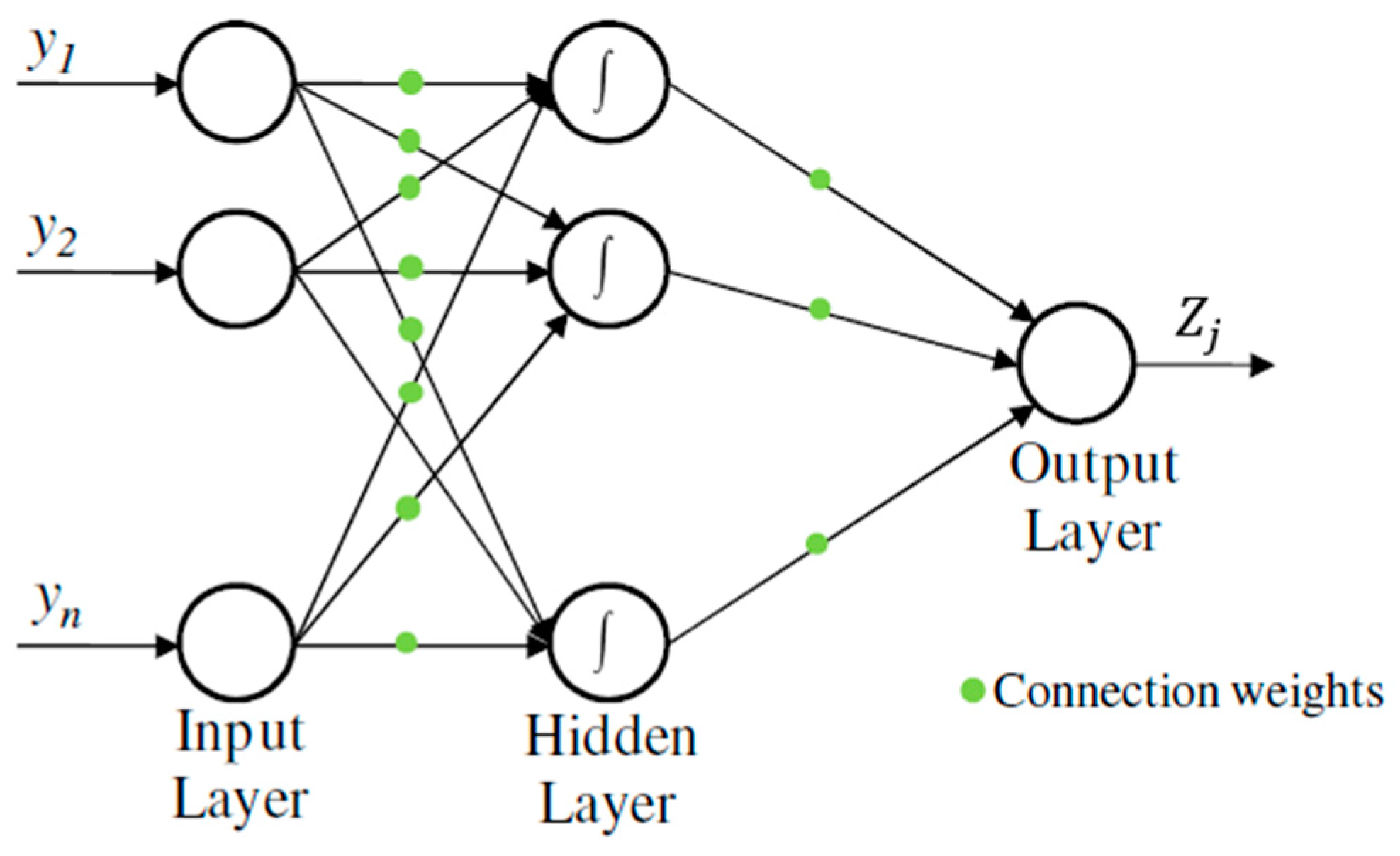
15]. Nodes are organized in different layers which are classified into input, hidden and output layers. Connections between neurons are established with one or more neurons of the following layers only. Each connection between neurons has a weight, which represents the importance of the preceding neuron in the result of the actual one.
Source nodes in the input layers supply the input vector, also called activation pattern, which will turn into the input signal for the neurons in the hidden layer. Each neuron receives a series of data from the preceding layer neurons and transforms them locally using an activation or transfer function and sends the result to one or more nodes in the following layer. The bias is used to shift value of the activation function for the next layers and consequently enhance the flexibility of the network. When the signal has been treated by all layers, the signal given by the last one, the output layer, constitutes the response of the network to the given input [
16]. A graphical representation of a MLP is shown in
Figure 1.
Mathematically a neuron of the MLP neural network can be modeled as Equation (1):
where
is the connection weight from neuron
to neuron
. While
is the input value from each neuron
,
is the output value of neuron
, after the application of
, the activation function of the node, which transforms the input locally.
In order to adopt the structure of the function embedded in the data, a learning algorithm is needed for training the network. This is performed by providing a set of the most representative inputs and their corresponding outputs; the learning algorithm is used then to change the values of the weights of the network. The learning algorithm is one of the key features in the performance of the neural network [
17]. Systems of neural networks can be used as reconstructors in the field of adaptive optics [
7].
2.2. Time Series Clustering
In order to study the characteristics of the reconstructors used in adaptive optics, different ways of networks data analysis were considered. As data changes in time, they were treated as time series. Since the analysis as univariate time series models or vectorial time series models turned out not to be the most appropriate, the usage of tools such as time series clustering became mandatory.
Self-Organising Tree Algorithm (SOTA) was first described by Dopazo and Carazo [
18] and is one from the wide range of existing algorithms for time series clustering. It is a clustering algorithm based on an unsupervised neural network with a binary tree topology. Specifically, the neural network is based on both Kohonen Self-Organizing Maps (SOM) [
19] and growing cell structure [
20]. This algorithm was developed for its use in recognition of gene patterns and, as advantage, it allows to work with big data sets with low computational cost [
21]. Furthermore, the advantages of this algorithm have been extensively discussed on previous works, where its performance, similarity and accuracy have been compared with the results provided by other clustering algorithm broadly used, such as Hierarchical Clustering or Self-Organizing Maps. These advantages are more remarkable as the data sets grow. For example, execution times for SOTA improve 85% over Hierarchical Clusterings and 64% over Self-Organizing Maps, when reaching data sizes of 5000 times series [
22].
The idea behind the algorithm uses as base the self-organized neural networks proposed by Kohonen that generates an output mapping which represents the estimation of the probability density function of the input data. This procedure is improved with the use of growing cell structure that allows to change the topology of the output map, increasing it in regions of higher density. SOTA algorithm implements this method with binary tree topology as output map, resulting on a hierarchical clustering algorithm with the robustness of a neural network.
SOTA algorithm is suitable for its use with several types of time series data [
23,
24,
25]. The implementation of this algorithm relays on the choice of a distance measurement of the time series data. Either
Euclidean distance or
Pearson correlation coefficient are considered. The selection of the best measurement is based on the aim of the clustering. For data with similar values on its properties,
Euclidean distance is recommended; on the other hand, the measurement of trends is done with
Pearson correlation coefficient [
21]. The steps for the algorithm, with the implementation of growing cell structure, are detailed below.
A cycle
of the algorithm is computed with the following steps:
Step 1: Computation of all distances between each profile vector or series vector to each external neurons;
Step 2: Selection of the winning cell between all the output neurons. The winning cell has minimum distance ;
Step 3: Update neuron
and its neighbors neurons as Equation (2) shows:
where
is the
-th cell vector at the cycle
and
the
th series vector. Also,
η is a decreasing term in time depending on the neuron that is updated and an initial number of iterations. This parameter is set in order to establish the convergence of the algorithm. The values for the factors
η were set at
,
and
which are set for the winning cell, the ancestors (the corresponding cell from the previous iteration) and the sisters cells (the output neurons that did not become the winning cell), respectively. Its election corresponds with the values originally set for the algorithm, which relies on the binary tree structure, and its topology [
18,
21].
When a cycle ends, the tree network is updated adding two neurons to the neuron with higher diversity, which is defined as the mean value of the distances between a neuron and each possible sequence linked to the neuron. It is defined in Equation (3):
where
is the number of possible sequences associated to the neuron
. The algorithm can be set to end when a number of epochs is reached or for certain values of diversity. Once the algorithm ended, the clustering corresponds to the topology of the trained network, as also happens in SOM algorithms.
In order to perform the clustering, a criteria is needed for the determination of the optimal number of clusters. Once the clustering is completed, internal measures of the partitions allow the determination of compactness, connectedness and separation of the cluster partitions. The Dunn index [
26] will be used as it characterizes both compactness and separation. Compactness assesses cluster homogeneity, which is characterized with the variance of elements in the same cluster, while separation quantifies the degree of separation between clusters.
The Dunn index is defined by Equation (4):
where
is the maximum distance between observations from the same cluster
. As it characterizes the relation of the minimum distance between observations from different clusters and the maximum distance between observations from the same cluster, Dunn index will have positive values and should be maximized. This measures the compactness of each cluster, and the separation between clusters, resulting on a value of the relation between them. The present research used the implementation of the SOTA algorithm and Dunn index of the package clValid (version 0.6-6) [
23] of the statistical software R (version 3.3.2) [
27].
2.3. Data Sets
In this work, we are considering two data sets from two reconstructors. For both of them, inputs are the same, simulated atmospheric data from four guide laser stars. The outputs corresponds with the response of each ANN reconstructor to the inputs.
The first set of data have the inputs and the outputs provided by CARMEN. The second set of data has the inputs and the outputs provided by a version of CARMEN which is currently in development. For this improved version, we update the neural network weights, using on-line training [
28]. This is done with real-time information about the current turbulence profile. Consequently, the weights for the trained network are updated continuously.
Both sets of data from the two reconstructor systems, will contain both input data for the neural networks and the outputs of the system. These elements have vectorial time series nature. With the purpose of analyzing the data, we will consider both input and output data together, so the resulting set of data will have concatenated all the time series.
In particular, the input data considered for this work of both data sets corresponds to the 144 centroids provided by a Shack-Hartmann Wave-front sensor [
29], which is set to measure the aberration of the light taken by a guide star. The centroids are determined for its horizontal and vertical coordinates, resulting on 288 data measurements. The measures are repeated each 2 ms, for a measurement time of 5 s, having a total of 2500 values for each series.
Some adaptive optics systems, as MOAO, uses a number of Shack-Hartmann sensor whose field of view overlap with that of the astronomical target in order to retrieve aberration information for the whole area of the integrated lightcone to the target, input data are measured for a total of 4 guide stars which corresponds the system CANARY-C2 [
30]. Input data are formed by the concatenation of the 4 sets of data. This leads to a total of 1152 time series that corresponds to the input data for both data sets. As well as input data was taken each 2 ms giving time series structure, so does the output data resulting on a vector of 288 time series.
2.4. Procedure
2.4.1. Objective of the Procedure
As the reconstructor CARMEN has good performance, it is expected that the improved version explained in
Section 2 will have good performance as well. In our case, despite the fact that the improved version seems to bring good results in the same terms as CARMEN [
8], the differences between them are the updates in time. Since the physical problem consists on the continuous variation of the atmosphere, it is expected that the on-line training of a network with new data provides more robustness over time. This is the reason a time structure comparison between CARMEN, which good performance we already know, and the time structure from the improved version is required.
With this procedure, the objectives are two-fold. First, we want to corroborate if exists any type of temporal structure in the temporal evolution of each value of the data. If it exists and is preserved in the outputs through the use of the network of CARMEN, we want to verify that in the case of the improved version, the temporal evolution can also be classified and preserved for the outputs of the network. Second, once the time structures are characterized and classified, we want to estimate the similarity between temporal structures of inputs and outputs and check if the performance over time in the reconstructor in development is comparable to the performance of CARMEN.
2.4.2. Treatment of the Data
As the aim of the procedure presented in this work is characterizing the behavior of a physical system with temporal evolution, the data sets considered will have input and output series concatenated in the same set.
It is, for the treatment of the data with this procedure, data should be presented to the algorithm as a set, which consists on time series that are to be classified and compared, assembled as sequence.
For any other data measurement that would be analyzed with this methodology, data should be treated in the same way, creating a dataset with the inputs and outputs of the system under study concatenated, as it allows an easier interpretation of the results and its subsequent analysis.
2.4.3. Clustering
Since input and output data are considered all together in the same set, without specifying distinctions, the application of a clustering algorithm will lead to distinguish temporal structures in the data, regardless it belongs to input or output data. Due to this property, the aim is to search if the inputs and outputs share similar time structure. Since the algorithm does not know the source of the data, it can cluster the output data alone (in one or more clusters) if output data do not share time structure with the other series, or it can be clustered in the same clusters as input data if the structure is similar.
This allows to confirm if input and output data shares similar time structure, but not only that, since in case of affirmative conclusion, this procedure establish a way to compare structures between clusterings. Then, characterization of the similarity of time structure between clusterings can be performed.
For the data sets considered, the election of SOTA as the clustering algorithm between all the available, as it was specified in
Section 2.2, is due to its computational simplicity for data sets of this magnitude. Time and complexity discussion of the algorithm can be found on [
21]. Also, its advantages in accuracy and performance over other algorithms [
22], justifies its choice as well.
2.4.4. Similarity of Temporal Structures
Usually, clustering comparison is performed in a one to one contrast, giving 0 or 1 if two series are in different or same cluster respectively, and averaging [
31,
32]. When the distance between clusters increases, the structure presents more differences, so we want to take this into account. In order to characterize “density patterns” in the clustering of each subset, the similarity value
Si, for series
i and
j classified in clusters
and
respectively, is defined in Equation (5):
Instead of giving 1 if the series belong to the same cluster, and 0 if not, we introduce the criteria: assigning a value that ranges from 0, if they are in different clusters at maximum distance, to 1, if they belong to the same cluster, and in other case, a proportional value to the distance between its clusters.
With this approach pattern structures in the input series can be recognized, if reproduced in the output series, even if they don’t belong to the same clusters. Also, this criterion allows to estimate a degree of similarity in the pattern structures from the input series and the output series.
3. Results
3.1. Procedure Results of the Data Set from CARMEN Reconstructor
Determination of the most adequate number of partitions for the first data set, is performed by means of the Dunn index calculation for different number of clusters. Results are shown in
Table 1.
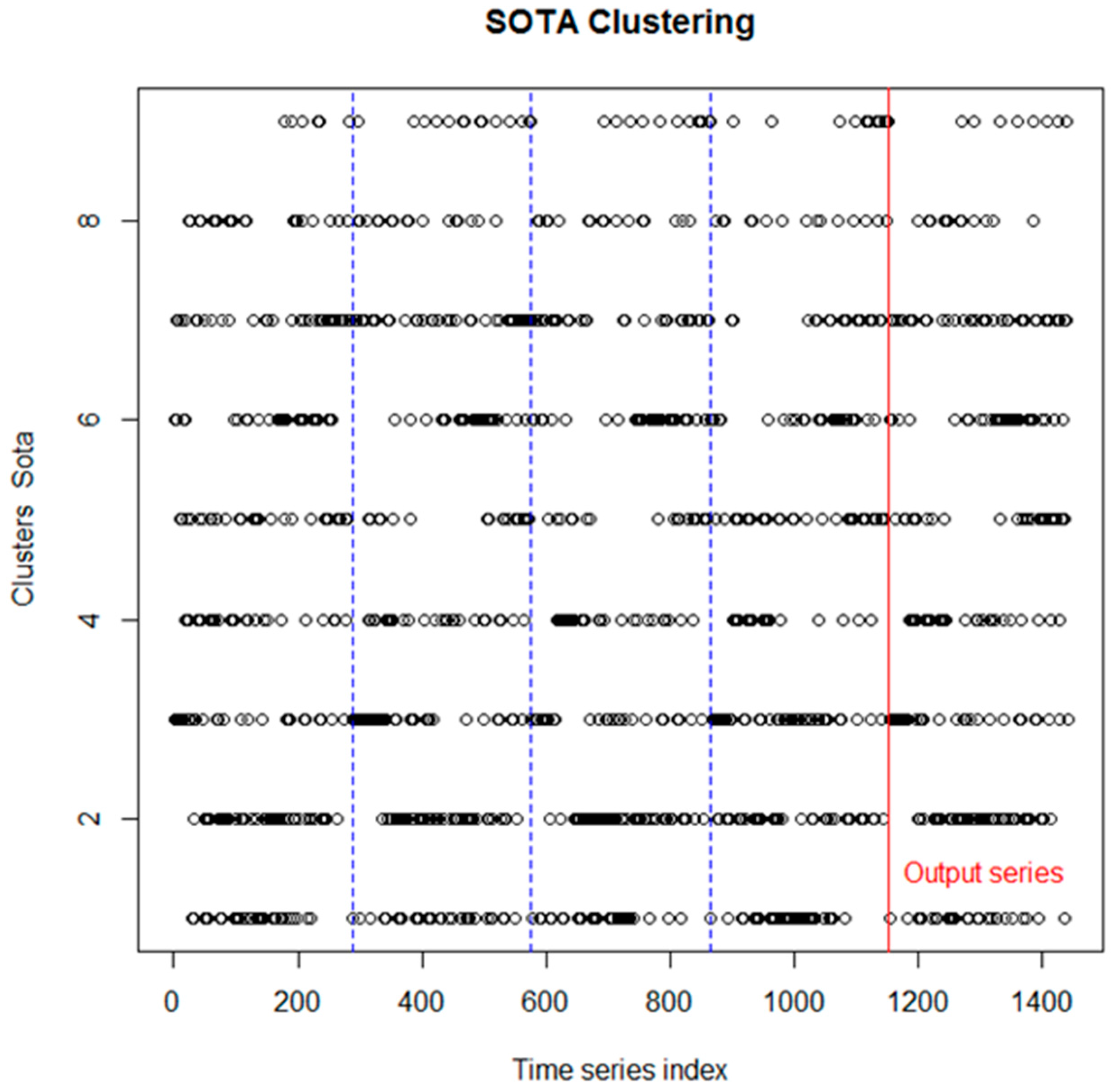
The best option for clustering the data seems to be nine partitions, since for ten partitions or higher, the value of Dunn index remains constant. This allows the clustering and the formation of binary tree structure by the algorithm with the given data.
Results of the clustering for each series from the first data set are shown in
Figure 2. As it was discussed above, the fact that the clustering algorithm recognizes similar time structure for inputs and outputs (by classifying the series from the outputs in the same clusters as the series from the inputs), shows that the physical system, in this case the neural network, preserves time structure within its application.
Once the first objective is confirmed, we use the previous results to characterize the similarity between temporal structures in input and output data. This will be presented by means of contrasting the structures in each subset of inputs and the set of outputs.
3.2. Procedure Results of the Data Set from Improved CARMEN Reconstructor
For the second data set, the procedure will be performed in the same way. Dunn index is shown in
Table 2.
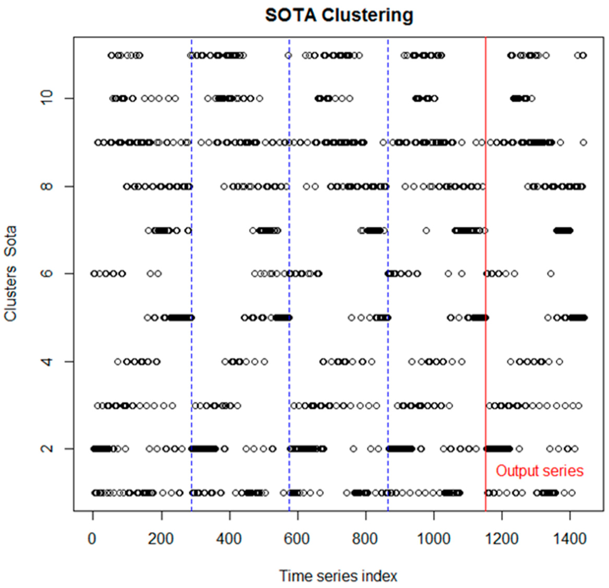
Since for more than 11 clusters, the Dunn index associated to this data remains constant, the most appropriate number of clusters, regarding to connectivity, corresponds to 11. Clustering is performed in all the subsets of series attached together, and the distribution in clusters of these series can be observed in the graphic of
Figure 3.
3.3. Similarity Results
For the first data set, the contrast between clustering from each subset of inputs and the subset of outputs is shown in
Table 3.
The measurement of the similarities for the second clustering is shown in
Table 4.
4. Discussion
For the original reconstructor, in average, the result is 82.67% of similarity between the structures of the clustering, very similar for the first three sets of inputs and slightly lower for the fourth. All the results, graphical and numerical, allow the characterization of the similarity, and in this case, support the hypothesis of preservation of time structure of the input series into the output series via the neural network system.
For the new system considered, as can be observed in
Figure 3, temporal structure of the series tend to be replicated in each subset of series, and the structure for the series belonging to the output subset is very similar to the structure of the series from the subsets of inputs. Since the density patterns in the distribution of series among the clusters is similar, the improved version of CARMEN preserves the temporal structure, as CARMEN does. In average, there is an 87.53% of similarity, and both numerical and graphical results leads to a high similarity of time structures between the inputs and the outputs of the system.
This procedure allowed us to characterize the high percentage of time structure preservation of both systems and conclude that the new version of the reconstructor is expected to perform satisfactorily, as the original does, when it gets implemented.
5. Conclusions
The procedure described in the present paper, was determined by the necessity of finding an adequate tool to describe the temporal structures in reconstructors for adaptive optics, where the robustness for temporal evolution is a relevant feature.
The goals of the procedure are to accomplish two aims; first, determining if exists correlation between temporal structures from inputs and outputs of any system with temporal evolution, and second, characterizing the similitude of these temporal structures. Both aims were checked in two applications with real data sets with positive results.
In this paper, the procedure was tested satisfactorily with data from two reconstructors and then, it is concluded that both systems are suitable for its implementation on real situations. Particularly, in CARMEN, that already had its good performance proven in previous works, resulted in finding temporal structure between its inputs and outputs. Also, this allowed us to characterize the similarity between time structure patterns.
Since the aberrations produced by the atmosphere are continuous and extremely fast, the idea in the development of the second reconstructor is its improvement in each time instant. As this is also the main difference from the original reconstructor, we wanted to find a similar time structure behavior between inputs and outputs, to corroborate that its performance over time is in the same terms as CARMEN.
Regarding the similarity values of time structure for the time series of inputs and outputs obtained, the procedure suggest that the second reconstructor will work correctly, at least when used for time intervals of 5 s, which is the time frame of the analyzed data. This encourage us to continue the work in the development of this type of recontructors and opens the possibility of its future implementation in telescopes.
Although this procedure is applied to data provided from ANNs, it can be used in any other physical system with temporal evolution where their robustness is relevant and its characterization is required. Consequently, the procedure allow us to test the suitability of the reconstructors before implementation on real applications. Additionally, although this procedure is presented here for an adaptive optics application, it is expected to perform the characterization of data, as long as the data has evolution in time, from several types of physical systems, for testing its suitability as well.


 ,
, 
