
Multilevel Integration Entropies: The Case of Reconstruction of Structural Quasi-Stability in Building Complex Datasets


1
Shenzhen Graduate School, Harbin Institute of Technology, Shenzhen 518055, China
2
Institute of Nuclear Sciences Vinča, University of Belgrade, Belgrade 11351, Serbia
3
Shenzhen Graduate School, Harbin Institute of Technology, Shenzhen 518055, China
*
Author to whom correspondence should be addressed.
Entropy 2017, 19(4), 172; https://doi.org/10.3390/e19040172
Submission received: 27 February 2017
/
Revised: 12 April 2017
/
Accepted: 14 April 2017
/
Published: 18 April 2017
Abstract
:The emergence of complex datasets permeates versatile research disciplines leading to the necessity to develop methods for tackling complexity through finding the patterns inherent in datasets. The challenge lies in transforming the extracted patterns into pragmatic knowledge. In this paper, new information entropy measures for the characterization of the multidimensional structure extracted from complex datasets are proposed, complementing the conventionally-applied algebraic topology methods. Derived from topological relationships embedded in datasets, multilevel entropy measures are used to track transitions in building the high dimensional structure of datasets captured by the stratified partition of a simplicial complex. The proposed entropies are found suitable for defining and operationalizing the intuitive notions of structural relationships in a cumulative experience of a taxi driver’s cognitive map formed by origins and destinations. The comparison of multilevel integration entropies calculated after each new added ride to the data structure indicates slowing the pace of change over time in the origin-destination structure. The repetitiveness in taxi driver rides, and the stability of origin-destination structure, exhibits the relative invariance of rides in space and time. These results shed light on taxi driver’s ride habits, as well as on the commuting of persons whom he/she drove.
1. Introduction
The omnipresent phenomenon of complexity permeates contemporary research topics in physical, social, biological, informational sciences, as well as the industry sectors, and it is followed by the explosion of large quantities of data about complex systems. Answering the question “How can we extract meaningful information from the data in order to decipher the challenges imposed by the complexity?” can get us closer to resolving problems about the properties of complex datasets and, accordingly, reconstructing the internal properties of complex systems. The initial steps toward solutions require the development of a methodology that would accurately detect the pertinent, intrinsic, dependencies of the elements of the dataset, under the assumption that dependencies embedded in a dataset lead toward building patterns of behavior at different aggregation levels of dataset elements.
In order to characterize the (in)distinguishability of substructures embedded in the dataset, we introduced the information entropy measures, to quantify the information that emerges from the built-in similarity relationships of dataset elements represented by the connectivity embedded at different levels of the hierarchical data structure. The structure of a dataset is mathematically represented as a simplicial complex, hence providing us the opportunity to apply the rich apparatus of algebraic topology [1]. Based on the Shannon information measure [2], we define the multi-dimensional entropies and depart from the hitherto research that relates the concepts of algebraic topology and information theory, such as the cohomological nature of information [3], persistent entropy [4,5], the graph’s topological entropy [6] or higher-order spectral entropy [7]. The introduced vector-like entropies capture the (in)distinguishability of different layers of the rigorously partitioned structure of the dataset and, further, indicate the way that the changes of data affect the internal structural relationships of the dataset. Hence, our objective is to relate the structure of a simplicial complex, via entropy measures, to the pattern formation of dependencies between aggregations of complex datasets.
Topological data analysis (TDA) [8,9,10,11] emerges as a powerful tool for the extraction of the shapes of large datasets, thus complementing conventional statistical methods for data analysis. Though the rapid advancement of TDA brings various tools under the umbrella of data analysis research, the rich conceptual repertoire of algebraic topology has not yet been exhausted. The most important tool of TDA is the persistent homology method [12,13], which is proven as useful in many real-world applications. The abundance of applications covers a broad range of phenomena in biological and medical science, like breast cancer research [14], brain science [15,16,17,18,19,20,21], biomolecules [22,23,24], evolution [25] and bacteria [26], followed by the applications in sensor networks [27,28], signal analysis [29], image processing [30], musical data [31], text mining [32], phase space reconstruction of dynamical systems [33,34], as well as complex networks related to either dynamics taking place on networks [35] or structural properties [36,37].
Originating from the same field of mathematics as TDA, i.e., algebraic topology, and based on the ideas of modeling complex social systems, R.Atkin developed the mathematical framework called Q-analysis [38,39,40] with the intention to capture versatile structural properties of social phenomena, as well as datasets emerging in these phenomena. The applications of Q-analysis span through different fields and problems, like studying the qualitative and quantitative structure of television programs [41], analysis of the content of newspaper stories [42], social networks [43,44,45,46], urban planning [47,48], relationships among geological regions [49], distribution systems [50], decision making [51], diagnosis of failure in large systems [52], controllability of dynamical systems [53] and the game of chess [54], to mention a few. These applications, and many others, express the usefulness of Q-analysis in data analysis; nevertheless, in most of the cases, it was applied to the analysis of small datasets suggesting possible inadequacy for handling the modern explosion of large datasets. Aside from recent applications of the concepts emerging from Q-analysis on higher-order structural properties of complex networks [55], an extension of Q-analysis concepts to larger datasets is still lacking.
The objects of interest that are built from the dataset are the same for the TDA and Q-analysis, that is convex polyhedra, called simplices, and their aggregation into simplicial complex [1], which builds the higher-dimensional discrete geometrical space. Nevertheless, the definitions of collections of simplices within simplicial complex are defined in rather different ways. The apparatus of TDA is rooted mostly on the homology groups, which are defined for the groups of the same-dimensional simplices called chain groups, where the chain represents a formal sum of the same-dimensional simplices. On the other hand, the Q-analysis method is grounded on building the chains of connectivity between multi-dimensional simplices through their multi-dimensional overlapping. Since the aggregations of simplices emerging from the Q-analysis method explicitly capture the versatility of relationships between simplices, and accordingly between the elements of the original complex dataset, we have defined multilevel integration entropies under the framework of Q-analysis.
We have calculated the multilevel integration entropies for the case of GPS coordinates (latitude and longitude) of a taxi driver’s pick up and drop off of passengers. Namely, this dataset is particularly convenient due to its different properties. First, the building of this particular dataset can be traced in time, since a taxi driver accumulates knowledge about visited locations. Second, without loss of generality, it turns out to be suitable for the clear introduction of the Q-analysis concepts and, hence, the interpretation of results, due to the origin/destination relationship. Third, this dataset can be interpreted from a two-fold point of view. From the taxi driver point of view, the cumulative aggregation of experience (or knowledge) builds a part of the so-called cognitive map [56]. Namely, as taxi drivers take passengers, they travel through the city environment and, hence, incrementally accumulate the experience about the origins and destinations they have visited. In that way, through the experience, a particular taxi driver builds a mental map (or cognitive map) [57]. Although there are different definitions of a cognitive map, for the purposes of the current research, we will accept a very general one: the cognitive map is a mental construct that we use to understand and know the environment [58]. Hence, the reason for building the cognitive map is that people store information about their environment, which they then use to make spatial decisions. Or in the broadest sense, the cognitive map is the cognitive apparatus that underlies...behavior [59]. The reason for choosing the broad definitions lies in the following: we are considering an abstract mind space built from the relationships between origins and destinations that has topological and combinatorial relationships, whereas the cognitive map may also store information about distances between places (hence, including some metrics), the routes and paths where people have traveled, the names of places and other information that can be learned from and about the environment. Hence, the abstract mental space of relationships between origins and destinations can be understood as a subset of the actual cognitive map and treated as the truncated cognitive map. On the other hand, the taxi drivers’ data are convenient for considering cognitive maps as the underlying space of behavior, especially since we know that they originate from the purposes that characterize the specificity of the work characteristics of the taxi drivers. Namely, the previous research in cognitive maps of taxi drivers showed that, due to the particularity of their jobs, they recover the urban spatial structure with higher accuracy than other social groups whose job is not related to traveling within the city [60] or that of novice taxi drivers [61].
From another point of view, the analysis of the datasets of a taxi driver’s GPS coordinates can be interpreted in the context of human mobility [62], as well. Namely, the research involving people commuting in an urban area attracted considerable attention [63,64], particularly due to the interest in the possible prediction of human mobility [65] (where entropy measures have been used in the research of limitations in the predictability of human mobility). Although our results can be interpreted either way, we restrict ourselves to the former one. The reason for this choice lies in the necessity that, if we want to examine human mobility, the data from more taxi drivers should be taken into consideration. Nevertheless, as will be shown, even the data from one taxi driver’s rides are enough for highlighting the patterns of behavior in time and space, on the one side, and to emphasize the characterization of intrinsic structural changes of dataset by introduced entropy concepts, on the other.
The case study of a taxi driver’s GPS datasets demonstrates that the methodology can be applied to a wide variety of real-world datasets, although further developments in building a more consistent research program in relation to the conventional topological data analysis remain to be developed.
2. Results
Our aim is to express the collection of elements of datasets in a holistic way as the integrated configuration of information [66,67], rather than as a simple collection of elements. In that way, the collection of elements of datasets builds the structure, which captures the patterns embedded within the dataset. This enables us to build a multidimensional structure of a simplicial complex and then analyze it using an appropriate apparatus grounded in algebraic topology. In the core of such an apparatus lies the methodology for the extraction of chains of connectivity between groups of elements in datasets.
2.1. Simplicial Complex in the Context of Case Study
We have considered the dataset obtained from the GPS coordinates of pick up and drop off recordings of one taxi driver who had 3623 rides, after data cleaning (see the Appendix), recorded during the period of three months. The city area is divided into square cells of equal size 2 km × 2 km each and labeled by numerals from 1 to 968. When the taxi driver picks up a passenger at the location that is within the cell i and drops off a passenger at the location that is within the cell j, we say that the taxi driver drove from origin i to the destination j. The information about drives from origins to destinations is stored in the origin-destination () matrix, where rows are associated with origins, columns are associated with the destinations, and the matrix elements are if the taxi driver had a ride from origin i to destination j, and otherwise. Building a simplicial complex (see the Appendix for a formal definition) from these data is straightforward: associate origins (rows) to simplices and destinations (columns) to vertices. In this way, we build the simplicial complex of origins and, accordingly, its conjugate complex is the simplicial complex of destinations; hence, we are provided with the two-fold reconstruction of the structure of a cognitive map, or in other words, a complex system of taxi driver’s rides.
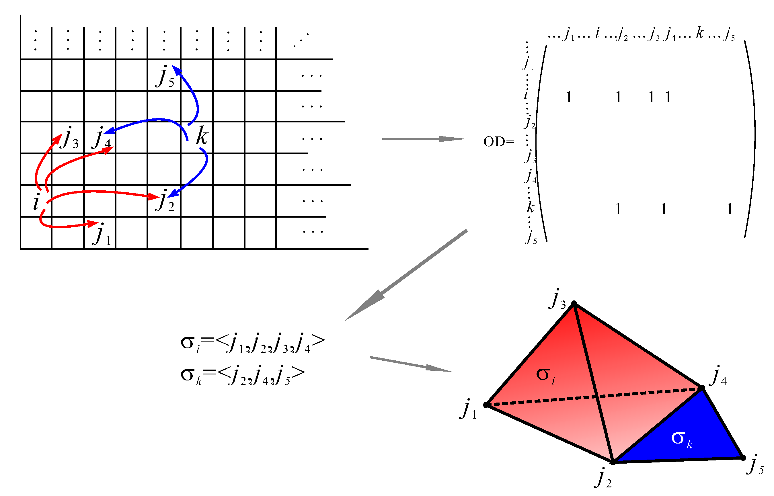
An example of the procedure of building a simplicial complex is illustrated in Figure 1 for the case when the taxi driver picked up passengers at the location within the cells i and k and dropped them off at destinations , , , and , , , respectively. The information about it is stored in the origin-destination () matrix where nonzero elements are associated with the entries , , , , , and . Hence, relating simplices to rows and vertices to columns, we identify two simplices and , represented geometrically as three-simplex and two-simplex, which share one-face.
Generally, the dataset of locations, which the taxi driver visited, is divided into two datasets: the set of origins X and the set of destinations Y, which are apparently overlapping. Taking into consideration that from one origin the taxi driver can, at different time moments, take rides to different destinations , then the rule “rides from origin to destination” is associated with the binary relation , which partitions a set of destinations Y into subsets, building the subset of the power set of Y [41,68]. Each element is associated with an element from the set , which is -related to them. For convenience, in order to make a distinction between an element from the set X and an element of the power set to which an element is -related, we will label the latter as . Although this distinction seems unnecessary, it makes an important conceptual step in our approach. Namely, whereas “” is just an element in the set X, the represents an integrated collection of elements generated by the -relation and, as such, labels the information of the aggregation of elements. In this way, the integrated collection of elements of dataset Y becomes an object of interest embodied in the element of another set X, hence introducing the technique of naming a collection of objects. In the example presented in Figure 1, simplex labels the integrated configuration of information, which emerged from the compilation of taxi driver rides from the cell i to cells , , , . In the first approximation, the knowledge of visiting any of the , , , cells cannot be separated from the knowledge of visiting all of them. Although due to the memory effect (like forgetting), it is possible in reality.
The elements of the set may overlap, since the taxi driver can have rides from different origins toward some of the same destinations. This property leads us to another partition of the dataset by focusing on the chains of connectivity between the elements of set X via their dependence on the elements of Y [38,39]. In order to extract the chains of connectivity within the dataset, we will reach for concepts of algebraic topology. We can represent each element of the set X by a convex polyhedron [1,69] defined with vertices and write it as:
whenever the matrix of relation has entry one at positions , with (like in the example in Figure 1). This q-dimensional polyhedron represents a q-simplex [1], and polyhedra among themselves may share subpolyhedra, called faces [1]. The collection of simplices together with all of their faces is called a simplicial complex [1], denoted by , and the notation means that the set X provided the names for simplices (i.e., ) and is called the set of simplices, whereas the set Y is the set of vertices that define simplices by the relation [68]. Generally, whether we first choose that the elements of set X are related to the elements of set Y, or vice versa, is rather arbitrary, since either the dataset or the context of the inquiry does not impose any constrains. Therefore, there are naturally two simplicial complexes related to the dataset: the first that we have already defined and the second, defined by the inverse of the -relation, , that is [69]. Accordingly, in the first, simplices are built by the integration of elements of Y into the subsets of Y and named by the elements of the set X, whereas the second simplicial complex is built by the integration of elements of X into the subsets of X and named by the elements of set Y. The simplicial complex is called the conjugate complex of simplicial complex . The dimension of simplicial complex is equal to the maximal dimension of all simplices.
The elements of the set may share different numbers of elements from Y, that is the faces shared by polyhedra can have different dimensions. Hence, when a p-simplex and an r-simplex share vertices, common to the sets of vertices and vertices that define and , respectively, we say that two simplices and share q-dimensional face or q-face [68] in the structure of . Two simplices and are said to be q-connected [68] if between them exists a chain of connection, such that every two adjacent simplices share at least a q-face. The relation of q-connectivity between simplices of is an equivalence relation, which partitions the simplicial complex , for any given q-value, into disjointed components. Note that the chains of q-connectivity are not the same as the formal sums of the elements of chain group [1]. Namely, the set of k-simplices forms the so-called chain group , with the addition as group operation, and the formal sum of a finite number of oriented k-simplices is a k-chain of simplices. Hence, all members of the k-chain have the same dimension, whereas the members of the q-connectivity chain may have different dimensions ranging from to q. Further, unlike the q-connectivity chain, which is defined due to the face-sharing property between simplices, the members of the k-chain do not have to share vertices.
The number of disjointed components for different q-values is stored in the entries of the Q-vector (or the structure vector) [55,68]:
The equivalence relation for different q-values partitions the simplicial complex into a sequence of simplicial complexes, where, for the decreasing q-values, each set is a subset of the subsequent set, or more precisely:
where is the dimension of a simplicial complex, and is the simplicial subcomplex at the q-level, containing simplices higher or equal to the dimension q. In this way, the natural filtration of the simplicial complex is defined, since the filtration parameter takes the values of the sequence of dimensions.
The origin/destination matrix is initially empty; the rides are arranged by the sequence of unevenly spaced temporal events , which are associated with the occurrences of rides, and if the taxi driver had a ride from origin i to the destination j at the moment , then the matrix element is increased by one (i.e., ). Note that, defined in this way, we build a sequence of nested simplicial complexes:
which resembles the persistent homology filtration [12], with the time as a parameter. Nevertheless, at this moment, our procedure is departing from the approach of persistent homology, since our interest is in the connectivity chains of a different kind, which are not (but can be) non-bounding cycles. Figure 2 illustrates the way of building the sequence of simplicial complexes and the structural changes encoded in the Q-vector entries, by adding new taxi rides in consecutive time moments. In the example presented in Figure 2, for convenience, simplices and vertices are labeled differently, although in our case study, the sets of origins and destinations are the same, hence having the same labels. From the example illustrated in Figure 2 at the moment , the taxi driver had a ride from origin b to the destination 3, which as a consequence has changed in the dimension of simplex , whereas at the moment , the taxi driver had a ride from the origin e to the destination 7, which as a consequence has change in the dimension of simplex . The changes in these time moment transitions affected q-levels 2 and 1.
2.2. Multilevel Integration Entropies
Within the structure of dataset , disjointed collections of simplices are embedded for a particular q-value, and hence, the probability of finding a connectivity class that emerges at the q-level is equal to . We define a integration entropy for each q-value as:
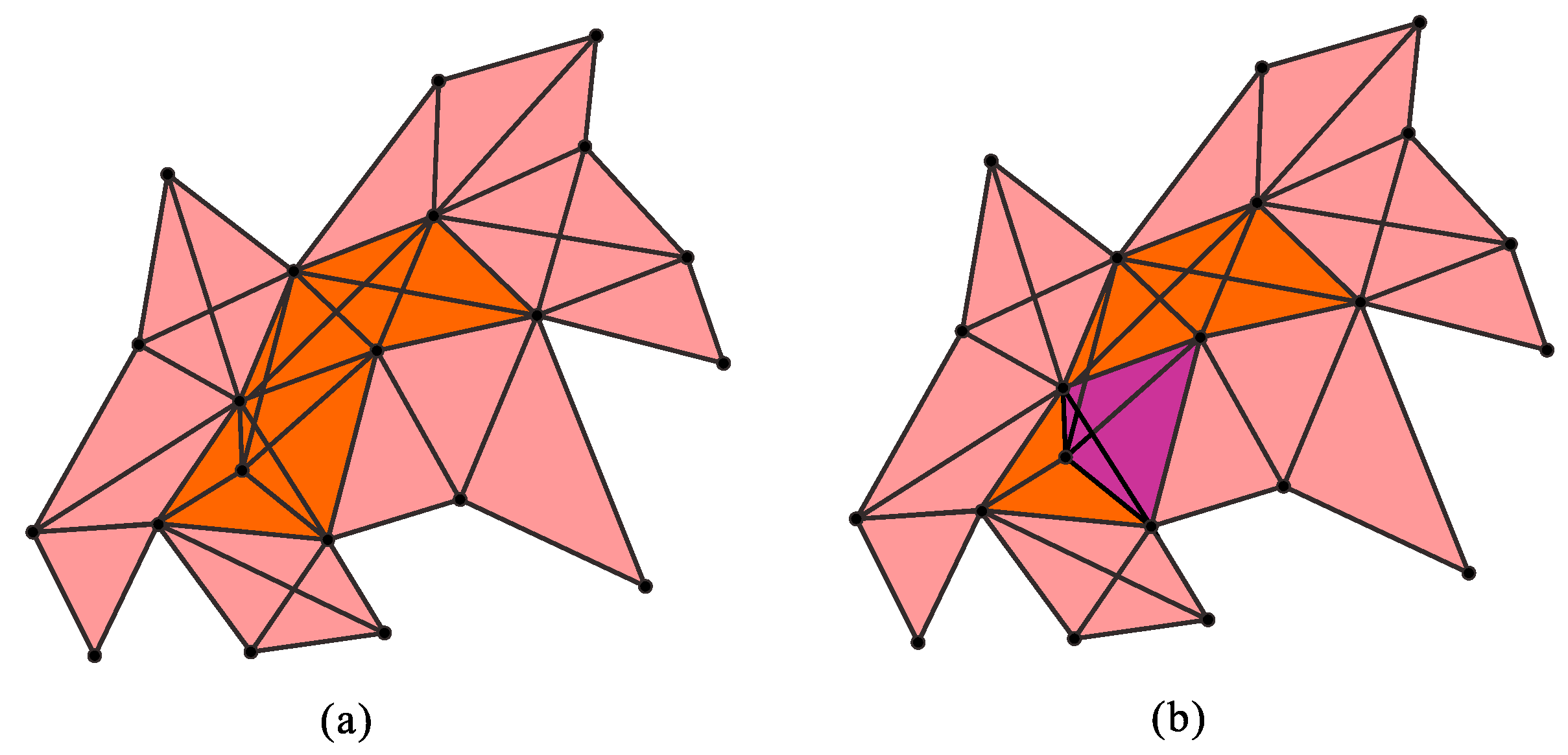
which measures the uncertainty of finding the q-connectivity class, or the indistinguishability of the collection of simplices for a q-value, and accordingly, the indistinguishability of the aggregation of the group of elements of datasets for a q-value. Clearly, . Figure 3a illustrates the way in which the connectivity class is embedded into the structure of a simplicial complex. If we have only one connectivity class , then , meaning that the collection of simplices is distinguishable for the q-value, or if we have connectivity classes, where N is the number of simplices at the q-level, then has maximal value. Note that is the vector quantity:
Since q-simplex appears at the levels q, , , ..., 1, 0, it is a part of some connectivity class at each of these levels. The property of embeddedness of a single simplex within the connectivity class within the simplicial complex is illustrated in Figure 3b, for one simplex and one connectivity class. We define the probability that a simplex appears in i-th connectivity class at the q-level as:
where is the number of simplices in the i-th connectivity class at the q-level, is the total number of simplices at the q-level, and the probability is normalized
We define a participation in an integration entropy measure, which quantifies the uncertainty to find a simplex at the q-level, or in other words, the (in)distinguishability of simplices at the q-level:
and this quantity is also vector-like:
Two limiting cases emerge for the entropy value : (1) at the q-level, only one connectivity class exists, then ; and (2) at the q-level, connectivity classes exist, and each contains only one simplex, then .
The amount of new information under the update of relations between datasets is different for two entropies. The entropy can be changed only if at the q-level, the updated data structure leads toward merging, splitting or adding new connectivity classes, regardless of the number of simplices that form them. On the other hand, the amount of new information of may either increase or decrease by changing the number of simplices in connectivity classes, together with the merging, splitting or adding of new connectivity classes. For every q, .
2.3. Results of the Calculations
The values of vector entries of entropy , for the simplicial complex and its conjugate calculated at temporal events , when the taxi driver had a ride, are presented in Figure 4a,b, respectively, and the values of vector entries of entropy for simplicial complex and its conjugate calculated at temporal events t when the taxi driver had a ride are presented in Figure 5a,b, respectively. From Figure 4 and Figure 5, we notice that the information about the aggregation of simplices and (in)distinguishability of simplices at different sub-structural levels is changing as new data are added. The first notable characteristic is that the q-level for which entropies are maximal (indicated by different shades of red) is increasing in time. Specifically, the values of maximal entropy in the case of the conjugate complex (built by the destination simplices) are higher for both entropies and . What clearly distinguishes the results for and is the zone of smaller entropy values for lower q-levels, indicated by the blue color in Figure 4 and Figure 5. Whereas the width of the zones of lower values for the simplicial complex and its conjugate are increasing over time, for the entropy , this is not the case. The behavior can be interpreted in the following way: with each new ride, the change of the simplex’s (either origin or destination) dimension shifts that simplex to a higher dimension fostering the distinguishability between simplices, and hence, the width of the zone of lower entropy values increases. Nevertheless, the connectivity of the group of simplices is less affected by the simplex’s changes due to the addition of new rides.
Nevertheless, a closer look at all four figures suggests that differences in entropy values at the same q-level and at two successive time moments are not too different. Hence, the calculation of similarity between entropies at two successive moments, performed for the whole time period, may shed light on understanding the transitions in data structure under the changes of entropy. The comparison of vector-like quantities that characterize the simplicial complex can be performed in different ways, for example by finding the critical dimension [47,48] or calculation of the cosine of an angle between two vectors [38]; we have chosen the latter one for the following reasons. Namely, we are interested in the changes of the structure of the dataset under the filtration of the simplicial complex through the successive time steps by calculating the entropies of the nested sequence of simplicial complexes. Hence, we want to track changes that emerge at different q-levels and that affect the overall structural changes of the simplicial complex. Therefore, for the comparison between entropies at two successive moments, we calculate:
and the same for the , and the norm is Euclidean:
and:
where . Hence, the coefficient , which we will call the entropy structural coefficient, takes the value of , with being the angle between the vectors and . The values of range from zero to one, where two entropy vectors are identical, in the latter case. For the convenience of the analysis of the results, the is labeled by and for and , respectively.
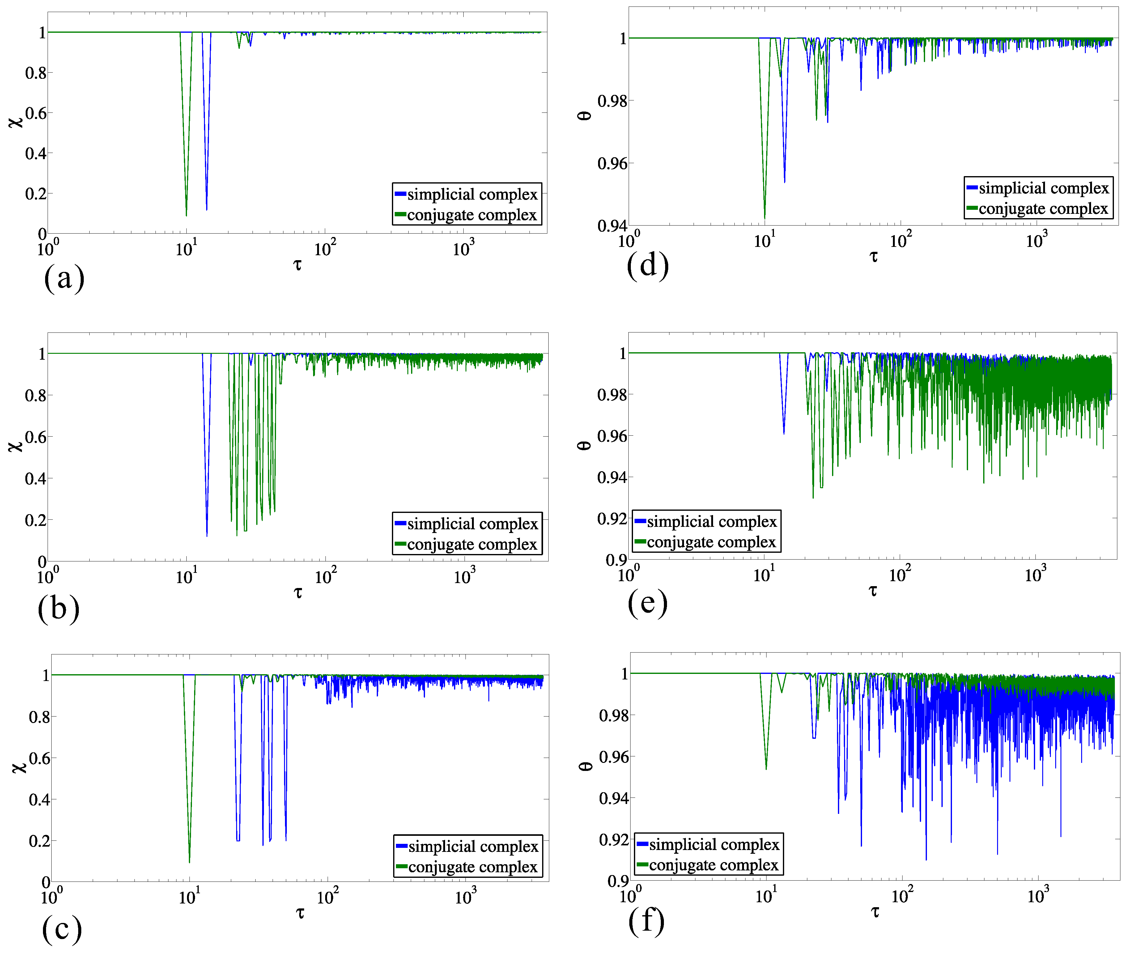
The values of entropy structural coefficient calculated between entropies and for a sequence of pairs of successive moments (labeled in graphics by ), for the simplicial complex and its conjugate, are presented in Figure 6a. After the initial significant differences in entropies, the transitions between two structures settles down close to the value , indicating the steady transitions. Similar behaviors appear in the case of the values of the entropy structural coefficient , calculated between entropies and for two successive moments , as is presented in the Figure 6d, for the simplicial complex and its conjugate. Although the behavior is similar, in the sense that the transitions settle down close to , the moment when steady transitions start occurs later.
Although the above results, for either or , indicate a certain regularity in achieving the relatively steady state of transitions in the structure of data, it is still necessary to verify to what extent the process of building the data structure carries the property of randomness. Therefore, we used the randomized datasets as the null hypothesis and compared it with the real-world dataset. The randomization procedure is performed in two ways, wherein the method of complex formation is the same as for the original data. Namely, in the first way, at each successive moment, the origin is the same as in the original data, whereas the destination is chosen randomly, and the simplicial complex is updated. In the second way, at each successive moment, the origin is chosen randomly, and the destination is the same as in the original data for a particular moment. In this way, we have built two sequences of simplicial complexes, calculated the entropies, and compared them with the results for the original data. Figure 6b,e presents the values of and , respectively, when the origins are from the original dataset and the destinations are randomized, whereas in Figure 6c,f, the values of and are presented, respectively, when the destinations are from the original dataset and the origins are randomized. All four figures indicate the significant difference with respect to the non-randomized data, though the entropy displays more robustness to the randomization. These results suggest the existence of regularity in building the simplicial complexes from datasets and accordingly regularity in building the taxi driver’s cognitive map. It practically means that, for example, the set of destinations toward which the taxi driver travels from one particular origin changes occasionally; the similarity between origins due to the shared common destinations is rather stable; and the groups of origins formed with respect to the similarity of shared destinations build a nonrandom structure.
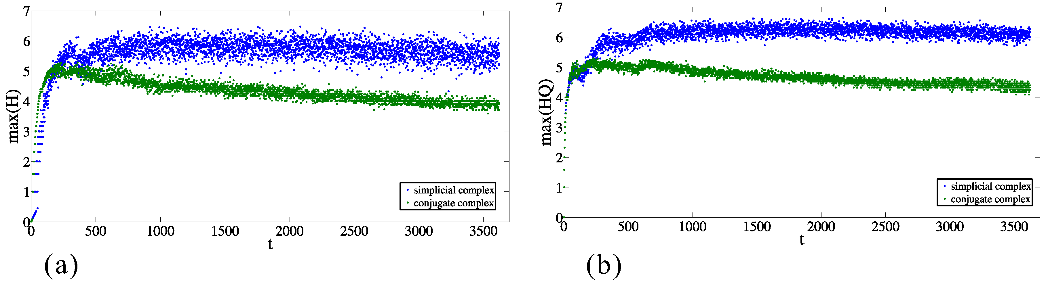
The discrepancy from random behavior is also obvious from the comparison between the maximal values of entries of entropies ( and ) for each moment in the original data and in the case of the randomized sets (as is explained above). Figure 7a,b presents the maximal values of and , respectively, for the simplicial complex and its conjugate. In both cases, in the majority of time moments, the maximal values are between and , and the maximal value for the conjugate complex is larger than for the simplicial complex. The same relationship is preserved when the origins are from the original dataset and the destinations are randomized (see Figure 8a,b, nevertheless the values are significantly different. In the case when the destinations are from the original dataset and the origins are randomized (Figure 9a,b), the results indicate complete discrepancy with respect to the original data.
3. Discussion
Herein, we have presented extensions of two data analysis methodologies (topological data analysis and Q-analysis), both originating from algebraic topology. For the case of the taxi driver’s origin-destination dataset, we have shown that the calculation and comparison of vector-like integration entropy measures lead toward detecting patterns in the generation of the dataset. Although the topological data analysis’ and the Q-analysis’ objects of interest, built over the dataset, are simplices, whose aggregation builds the topological structure of simplicial complex, the extraction of mesoscopic structures that carry the information about the shape of the dataset is different, and hence, the two methodologies complement each other. In this work, we have studied the emergence of mesoscopic structures defined within the framework of Q-analysis, that is the chains of multidimensional connectivity, and thus, shifted the focus of interest from the changes of homological objects (i.e., higher-dimensional holes) to the rigorously-defined structures built by the multidimensional collections of simplices. The partition of the simplicial complex of data into the hierarchy of sub-complexes proved to be suitable for the introduction of two multidimensional entropy measures for the comparison of structural changes of the dataset, which originate from the changes at different hierarchical levels. Particularly, the taxi driver’s origin-destination dataset comparison, between vector-like entropy measures for two consecutive rides, reveals steady behavior in transitions between two consecutive structures, unlike the case of a randomized dataset. Although the previously built cognitive map of the taxi driver is unknown to us, these results indicate that, after initial building, the core of accumulated origin-destination structure adds additional knowledge and leads toward the sporadic small changes in the structure. In other words, after some time, the taxi driver mostly has rides between previously known origins and destinations. From the analysis of such samples, we may conclude that the gross of the taxi driver’s rides are repetitive and relatively invariant in space and time. That is, whenever the taxi driver takes a new ride, it is likely that he/she already rode this ride before, rather than from a new origin toward a new destination. The cause of this kind of behavior can be either in the habit of the taxi driver to take rides between well-known origins and destinations to him/him, or the sample of persons whom he/she drove are inclined to follow a similar pattern, or the coupling between the two causes.
4. Conclusions and Future Work
It has been shown that the structure of datasets represented by a simplicial complex can be partitioned into the stratified sequence of rigorously-defined meso-structures, which are themselves simplicial complexes. The changes of the dataset affect the structure at different strata and, accordingly, are followed by the (dis)integration of meso-structures. In other words, the changes of the structure of datasets are followed by the changes of information at different strata of the dataset. The introduction of vector-like multi-level integration entropy measures proved to be useful for quantifying the information gain/loss, when meso-structures either join or disjoin. Hence, the comparison between multi-level integration entropies before and after the changes sheds light on the overall changes of the dataset structure caused by the (dis)integration of parts emerging at different levels.
Here, the calculations of comparisons between multi-level integration entropies suggest that the taxi driver’s behavior is repetitive; hence, in accordance with the results of the recent study [70], the taxi drivers’ learning of new spatial information with respect to the existing knowledge is rather poor. Nevertheless, in the context of datasets related to taxi drivers, the application will be extended to the larger group of taxi drivers, in the course of addressing the issues related to discovering the patterns of human mobility in an urban area [64,65]. Furthermore, future research may shed light on capturing the relationships between cognitive maps and commuting behavior in an urban environment and contribute to the further understanding of human mobility.
The results presented in this paper contribute to the research in spatial mental models in the sense introduced by B. Tversky [71]. We did not interview the taxi driver to acquire his spatial knowledge or the origin-destination relationships; nevertheless, from the repetitiveness of his behavior and accumulated knowledge, we may assume that he built the spatial mental model of origins and destinations. Although this assumption is rather strong, it provided us with an indirect approach to the research of building the spatial mental model.
Although in this study we limit ourselves to one specific dataset, the proposed method falls into the broader context of research in complex systems. Specifically, since different simplicial complexes can be obtained from complex networks, the calculation of proposed entropy measures may reveal additional insights into the evolution of complex networks in general and add a deeper understanding of the mechanisms that govern complex network building.
In the present paper, we address the importance, as well as usefulness, of methods that transcend homology-based tools and propose another strand of research in extracting significant and meaningful information from real datasets. The flexibility of our approach makes it suitable for the analysis of datasets of different sizes. Namely, since the method can be applied to small datasets, as well, it may serve as the bridge between large dataset and small dataset analysis.
Acknowledgments
The authors acknowledge support from the National Nature Science Foundation Committee (NSFC) of China under Project No. 61573119 and a Fundamental Research Project of Shenzhen under Projects No. JCYJ20120613144110654. and No. JCYJ20140417172417109, as well as Joyce G. Webb for editing.
Author Contributions
Slobodan Maletic designed the research, prepared the dataset and performed calculations. Slobodan Maletic and Yi Zhao analyzed the data and interpreted the results. Both authors wrote, reviewed and approved the manuscript.
Conflicts of Interest
The authors declare no conflict of interest.
Appendix A.
Appendix A.1. Simplicial Complex
A set of vertices , together with the set of subsets of this vertex set, called the set of simplices, defines a simplicial complex K [1]. Each subset called the q-simplex is uniquely defined by vertices, and the simplicial complex K is closed under the formation of subsets in the sense that any subset of a simplex from K is also a simplex from K. A p-simplex, which is defined by the subset of vertices of q-simplex , is called a p-face of the simplex . The dimension of simplicial complex K is the highest value of D for which is a simplex in K. Simplicial complex K is geometrically represented as a collection of convex polyhedra glued along the common faces, where a q-simplex is represented by a convex polyhedron with vertices.
Take two finite sets and and the binary relation between them (which by some rule, associates the elements of one set with the elements of another), then we can build two simplicial complexes. In the first one, as the vertex set may be taken , and a subset of vertices defines a q-simplex if, and only if, there exists at least one element , which is in the relation with each of these vertices [39,69]. We will denote the q-simplex, built in this way, by , and the simplicial complex by . Reversing the roles of the vertex set and the simplex set, that is applying the inverse relation , we define the second simplicial complex, called the conjugate complex of complex .
The property that any sub-simplex of a simplex is also a simplex induces various levels of adjacency between simplices and, therefore, multiple levels of connectivity between collections of simplices. Two simplices are q-near if they share a q-dimensional face [68], and hence, they are also , , ..., one- and zero-near. The collection of simplices in which any pair of simplices is connected by a chain of simplices where a pair of consecutive simplices is q-near is called the q-connected component. More formally, two simplices and are connected by the chain of q-connectivity [68] if there is a sequence of simplices such that any two consecutive simplices are at least q-near and . Note that if two simplices and are q-connected, they are also , , ..., one and zero-connected in K, due to the q-nearness property.
The q-connectivity between simplices induces an equivalence relation on simplices of a complex K, since it is reflexive, symmetric and transitive. This equivalence relation will be denoted by , so that:
Let be the set of simplices in K with dimensions greater than or equal to q, then partitions into equivalence classes of q-connected simplices. These equivalence classes are members of the quotient set , and they are called the q-connected components of K [39]. Every simplex in a q-component is q-connected to every other simplex in that component, but no simplex in one q-component is q-connected to any simplex on a distinct q-connected component. The cardinality of is denoted and is the number of distinct q-connected components in K. The value is the q-th entry of the so called Q-vector [39,55] (or first structure vector [68]), an integer vector with the length . The values of the Q-vector entries are usually written starting from the number of connected components for the largest dimension in descending order, i.e.,
The equivalence relations of q-connectivity partitions simplicial complex K into the sequence of nested simplicial sub-complexes, that is the filtration of simplicial complex K under the change of parameter q:
Furthermore, the values of Q-vector entries are equal to the zeroth-order Betti number [1] for each filtration stage.
Appendix A.2. Data Preparation
Taxi driver’s GPS data coordinates are recorded and collected within the time period of three months in Shenzhen City, China, during which the taxi driver had 4321 rides, and after data cleaning, 3623 rides were used in our calculations. In order to build matrices that capture rides from origins to destinations, the area of Shenzhen is covered by the rectangular grid of 968 cells 2 km × 2 km each. Due to the erroneous GPS coordinate recordings, part of the dataset is deleted leaving approximately of the rides in the initial dataset. The incorrect GPS recordings included the following faults either for origin or destination coordinates, or both:
- (1)
- appearance of zero values at the places of latitude and longitude coordinates;
- (2)
- the recordings of some rides were repeating;
- (3)
- the latitude and longitude coordinates of some rides are (far) out of the city border.
The cells on the grid are labeled by the numerals from 1 to 968, starting from the bottom left corner, and accordingly, the origin/destination matrix of the size is built. Whenever the origin has latitude and longitude coordinates that fall in the cell and destination has the latitude and longitude coordinates that fall in the cell , the matrix entry is increased by one.
Although we have performed calculations on the dataset of one taxi driver, the same procedure for data preparation, as well as the same coverage of the city area by rectangular grid of cells can be applied for the extraction of behavioral patterns of other taxi drivers.
References
- Munkres, J.R. Elements of Algebraic Topology; Addison-Wesley Publishing: Menlo Park, CA, USA, 1984. [Google Scholar]
- Shannon, C.E. A mathematical theory of communication. Bell Syst. Tech. J. 1948, 27, 379–423. [Google Scholar] [CrossRef]
- Baudot, P.; Bennequin, D. The Homological Nature of Entropy. Entropy 2015, 17, 3253–3318. [Google Scholar] [CrossRef]
- Chintakunta, H.; Gentimis, T.; Gonzalez-Diaz, R.; Jimenez, M.-J.; Krim, H. An entropy-based persistence barcode. Pattern Recognit. 2015, 48, 391–401. [Google Scholar] [CrossRef]
- Merelli, E.; Rucco, M.; Sloot, P.; Tesei, L. Topological Characterization of Complex Systems: Using Persistent Entropy. Entropy 2015, 17, 6872–6892. [Google Scholar] [CrossRef]
- Tadić, B.; Andjelković, M.; Šuvakov, M. The influence of architecture of nanoparticle networks on collective charge transport revealed by the fractal time series and topology of phase space manifolds. J. Coupled Syst. Multiscale Dyn. 2016, 4, 30–42. [Google Scholar] [CrossRef]
- Maletić, S.; Rajković, M. Combinatorial Laplacian and entropy of simplicial complexes associated with complex networks. Eur. Phys. J. ST 2012, 212, 77–97. [Google Scholar] [CrossRef]
- Lum, P.Y.; Singh, G.; Lehman, A.; Ishkanov, T.; Vejdemo-Johansson, M.; Alagappan, M.; Carlsson, J.; Carlsson, G. Extracting insights from the shape of complex data using topology. Sci. Rep. 2013, 3, 1236. [Google Scholar] [CrossRef] [PubMed]
- Carlsson, G. Topology and data. Bull. Am. Math. Soc. 2009, 46, 255–308. [Google Scholar] [CrossRef]
- Epstein, C.; Carlsson, G.; Edelsbrunner, H. Topological data analysis. Inverse Probl. 2011, 27, 120201. [Google Scholar]
- Edelsbrunner, H.; Harer, J. Computational Topology: An Introduction; American Mathematical Society: Providence, RI, USA, 2010. [Google Scholar]
- Edelsbrunner, H.; Harer, J. Persistent homology—A survey. Contemp. Math. 2008, 453, 257–282. [Google Scholar]
- Zomorodian, A.; Carlsson, G. Computing persistent homology. Discret. Comput. Geom. 2005, 33, 249–274. [Google Scholar] [CrossRef]
- Nicolau, M.; Levine, A.J.; Carlsson, G. Topology based data analysis identifies a subgroup of breast cancers with a unique mutational profile and excellent survival. Proc. Natl Acad. Sci. USA 2001, 108, 7265–7270. [Google Scholar] [CrossRef] [PubMed]
- Nielson, J.L.; Paquette, J.; Liu, A.W.; Guandique, C.F.; Tovar, C.A.; Inoue, T.; Irvine, K.-A.; Gensel, J.C.; Kloke, J.; Petrossian, T.C.; et al. Topological data analysis for discovery in preclinical spinal cord injury and traumatic brain injury. Nat. Commun. 2015, 6, 8581. [Google Scholar] [CrossRef] [PubMed]
- Petri, G.; Expert, P.; Turkheimer, F.; Carhart-Harris, R.; Nutt, D.; Hellyer, P.J.; Vaccarino, F. Homological scaffolds of brain functional networks. J. R. Soc. Interface 2014, 11, 20140873. [Google Scholar] [CrossRef] [PubMed]
- Lee, H.; Kang, H.; Chung, M.K.; Kim, B.N.; Lee, D.S. Persistent brain network homology from the perspective of dendrogram. IEEE Trans. Med. Imaging 2012, 31, 2267–2277. [Google Scholar] [PubMed]
- Singh, G.; Memoli, F.; Ishkhanov, T.; Sapiro, G.; Carlsson, G.; Ringach, D.L. Topological analysis of population activity in visual cortex. J. Vis. 2008, 8, 1–18. [Google Scholar] [CrossRef] [PubMed]
- Dabaghian, Y.; Mémoli, F.; Frank, L.; Carlsson, G. A topological paradigm for hippocampal spatial map formation using persistent homology. PLoS Comput. Biol. 2012, 8, e1002581. [Google Scholar] [CrossRef] [PubMed]
- Arai, M.; Brandt, V.; Dabaghian, Y. The Effects of Theta Precession on Spatial Learning and Simplicial Complex Dynamics in a Topological Model of the Hippocampal Spatial Map. PLoS Comput. Biol. 2014, 10, e1003651. [Google Scholar] [CrossRef] [PubMed]
- Bendich, P.; Marron, J.S.; Miller, E.; Pieloch, A.; Skwerer, S. Persistent homology analysis of brain artery trees. Ann. Appl. Stat. 2016, 10, 198–218. [Google Scholar] [CrossRef] [PubMed]
- Yao, Y.; Sun, J.; Huang, X.; Bowman, G.R.; Singh, G.; Lesnick, M.; Guibas, L.J.; Pande, V.S.; Carlsson, G. Topological methods for exploring low-density states in biomolecular folding pathways. J. Chem. Phys. 2009, 130, 144115. [Google Scholar] [CrossRef] [PubMed]
- Krishnamoorthy, B.; Provan, S.; Tropsha, A. A Topological Characterization of Protein Structure. Data Min. Biomed. Part IV 2007, 7, 431–455. [Google Scholar]
- Xia, K.; Wei, G.-W. Persistent homology analysis of protein structure, flexibility, and folding. Int. J. Numer. Methods Biomed. Eng. 2014, 30, 814–844. [Google Scholar] [CrossRef] [PubMed]
- Chan, J.M.; Carlsson, G.; Rabadan, R. Topology of viral evolution. Proc. Natl. Acad. Sci. USA 2013, 110, 18566. [Google Scholar] [CrossRef] [PubMed]
- Ibekwe, A.M.; Ma, J.; Crowley, D.E.; Yang, C.-H.; Johnson, A.M.; Petrossian, T.C.; Lum, P.Y. Topological data analysis of Escherichia coli O157: H7 and non-O157 survival in soils. Front. Cell. Infect. Microbiol. 2014, 4, 122. [Google Scholar] [CrossRef] [PubMed]
- De Silva, V.; Ghrist, R. Coordinate-free Coverage in Sensor Networks with Controlled Boundaries via Homology. Int. J. Robot. Res. 2006, 25, 1205–1222. [Google Scholar] [CrossRef]
- De Silva, V.; Ghrist, R. Coverage in sensor networks via persistent homology. Algebraic Geom. Topol. 2007, 7, 339–358. [Google Scholar] [CrossRef]
- Perea, J.A.; Harer, J. Sliding windows and persistence: An application of topological methods to signal analysis. Found. Comput. Math. 2015, 15, 799–838. [Google Scholar] [CrossRef]
- Carlsson, G.; Ishkhanov, T.; de Silva, V.; Zomorodian, A. On the local behavior of spaces of natural images. Int. J. Comput. Vis. 2008, 76, 1–12. [Google Scholar] [CrossRef]
- Sethares, W.A.; Budney, R. Topology of musical data. J. Math. Music 2014, 8, 73–92. [Google Scholar] [CrossRef]
- Wagner, H.; Dłotko, P.; Mrozek, M. Computational Topology in Text Mining. In Proceedings of the 4th International Workshop Computational Topology in Image Context, CTIC, Bertinoro, Italy, 28–30 May 2012; pp. 68–78. [Google Scholar]
- Maletić, S.; Zhao, Y.; Rajković, M. Persistent topological features of dynamical systems. Chaos 2016, 26, 053105. [Google Scholar] [CrossRef] [PubMed]
- Garland, J.; Bradley, E.; Meiss, J.D. Exploring the Topology of Dynamical Reconstructions. Physica D 2016, 334, 49–59. [Google Scholar] [CrossRef]
- Taylor, D.; Klimm, F.; Harrington, H.A.; Kramar, M.; Mischaikow, K.; Porter, M.A.; Mucha, P.J. Topological data analysis of contagion maps for examining spreading processes on networks. Nat. Commun. 2015, 6, 7723. [Google Scholar] [CrossRef] [PubMed]
- Carstens, C.J.; Horadam, K.J. Persistent Homology of Collaboration Networks. Math. Probl. Eng. 2013, 2013, 815035. [Google Scholar] [CrossRef]
- Horak, D.; Maletić, S.; Rajković, M. Persistent Homology of Complex Networks. J. Stat. Mech. 2009, 3, P03034. [Google Scholar] [CrossRef]
- Atkin, R.H. From cohomology in physics to q-connectivity in social sciences. Int. J. Man Mach. Stud. 1972, 4, 139–167. [Google Scholar] [CrossRef]
- Atkin, R.H. Combinatorial Connectivities in Social Systems; Birkhäuser Verlag: Stuttgart, Germany, 1977. [Google Scholar]
- Atkin, R.H. Mathematical Structure in Human Affairs; Heinemann: London, UK, 1974. [Google Scholar]
- Gould, P.; Johnson, J.; Chapman, G. The Structure of Television; Pion Limited: London, UK, 1984. [Google Scholar]
- Jacobson, T.L.; Yan, W. Q-Analysis Techniques for Studying Communication Content. Qual. Quant. 1998, 32, 93–108. [Google Scholar] [CrossRef]
- Seidman, S.B. Rethinking backcloth and traffic: Prespectives from social network analysis and Q-analysis. Environ. Plan. B 1983, 10, 439–456. [Google Scholar] [CrossRef]
- Freeman, L.C. Q-analysis and the structure of friendship networks. Int. J. Man Mach. Stud. 1980, 12, 367–378. [Google Scholar] [CrossRef]
- Doreian, P. Polyhedral Dynamics and Conflict Mobilization in Social Networks. Soc. Netw. 1981, 3, 107–116. [Google Scholar] [CrossRef]
- Doreian, P. Leveling coalitions as network phenomena. Soc. Netw. 1982, 4, 27–45. [Google Scholar] [CrossRef]
- Atkin, R.H.; Johnson, J.; Mancini, V. An analysis of urban structure using concepts of algebraic topology. Urban Stud. 1971, 8, 221–242. [Google Scholar] [CrossRef]
- Johnson, J. The q-analysis of road intersections. Int. J. Man Mach. Stud. 1976, 8, 531–548. [Google Scholar] [CrossRef]
- Griffiths, J.C. Geological Similarity by Q-Analysis. Math. Geol. 1983, 15, 85–108. [Google Scholar] [CrossRef]
- Duckstein, L. Evaluation of the Performance of a Distribution System by Q-Analysis. Appl. Math. Comput. 1983, 13, 173–185. [Google Scholar] [CrossRef]
- Duckstein, L.; Nobe, S.A. Q-analysis for modeling and decision making. Eur. J. Oper. Res. 1997, 103, 411–425. [Google Scholar] [CrossRef]
- Ishida, Y.; Adachi, N.; Tokumaru, H. Topological approach to failure diagnosis of large-scale systems. IEEE Trans. Syst. Man Cybern. 1985, 5, 327–333. [Google Scholar] [CrossRef]
- Casti, J. Polyhedral Dynamics and the Controllability of Dynamical Systems. J. Math. Anal. Appl. 1979, 68, 334–346. [Google Scholar] [CrossRef]
- Atkin, R.H. Multi-dimensional Structure in the Game of Chess. Int. J. Man Mach. Stud. 1972, 4, 341–362. [Google Scholar] [CrossRef]
- Maletić, S.; Rajković, M.; Vasiljević, D. Simplicial Complexes of Networks and Their Statistical Properties. Lect. Notes Comput. Sci. 2008, 5102, 568–575. [Google Scholar]
- Tolman, E.C. Cognitive maps in rats and men. Psychol. Rev. 1948, 55, 189–208. [Google Scholar] [CrossRef] [PubMed]
- Kitchin, R.M. Cognitive maps: What are they and why study them? J. Environ. Psychol. 1994, 14, 1–19. [Google Scholar] [CrossRef]
- Kaplan, S. Cognitive maps in perception and thought. In Image and Environment; Downs, R.M., Stea, D., Eds.; Aldine: Chicago, IL, USA, 1973; pp. 63–78. [Google Scholar]
- Tversky, B. Distortions in cognitive maps. Geoforum 1992, 23, 131–138. [Google Scholar] [CrossRef]
- Wakabayashia, Y.; Itohb, S.; Nagami, Y. The Use of Geospatial Information and Spatial Cognition of Taxi Drivers in Tokyo. Procedia Soc. Behav. Sci. 2011, 21, 353–361. [Google Scholar] [CrossRef]
- Giraudo, M.-D.; Peruch, P. Spatio-temporal aspects of the mental representation of urban space. J. Environ. Psychol. 1988, 8, 9–17. [Google Scholar] [CrossRef]
- Peng, C.; Jin, X.; Wong, K.-C.; Shi, M.; Liò, P. Collective Human Mobility Pattern from Taxi Trips in Urban Area. PLoS ONE 2012, 7, e34487. [Google Scholar]
- Brockmann, D.; Hufnagel, L.; Geisel, T. The scaling laws of human travel. Nature 2006, 439, 462–465. [Google Scholar] [CrossRef] [PubMed]
- González, M.C.; Hidalgo, C.A.; Barabási, A.-L. Understanding individual human mobility patterns. Nature 2008, 453, 779–782. [Google Scholar] [CrossRef] [PubMed]
- Song, C.; Qu, Z.; Blumm, N.; Barabási, A.-L. Limits of Predictability in Human Mobility. Science 2010, 327, 1018–1021. [Google Scholar] [CrossRef] [PubMed]
- Hull, C.L. The discrimination of stimulus configurations and the hypothesis of afferent neural interaction. Psychol. Rev. 1945, 52, 133–142. [Google Scholar] [CrossRef]
- Asch, S.E. Forming Impressions of Personality. J. Abnorm. Soc. Psychol. 1946, 41, 258–290. [Google Scholar] [CrossRef]
- Johnson, J.H. Some structures and notation of Q-analysis. Envniron. Plan. B 1981, 8, 73–86. [Google Scholar] [CrossRef]
- Dowker, C.H. Homology groups of relations. Ann. Math. 1952, 56, 84–95. [Google Scholar] [CrossRef]
- Woollett, K.; Maquire, E.A. The effect of navigational expertise on wayfinding in new environment. J. Environ. Psychol. 2010, 30, 565–573. [Google Scholar] [CrossRef] [PubMed]
- Tversky, B. Cognitive maps, cognitive collages, and spatial mental models. In Spatial Information Theory: A Theoretical Basis for GIS; Frank, A.U., Campari, I., Eds.; Springer-Verlag: New York, NY, USA, 1993; pp. 14–24. [Google Scholar]
Figure 1.
An example of simplicial complex construction from the taxi driver dataset when the city is divided into the grid of cells in the case when the taxi driver picked up passengers at the location within the cells i and k and dropped them off at destinations , , , and , , , respectively.
Figure 1.
An example of simplicial complex construction from the taxi driver dataset when the city is divided into the grid of cells in the case when the taxi driver picked up passengers at the location within the cells i and k and dropped them off at destinations , , , and , , , respectively.

Figure 2.
An example of updating the simplicial complex of origins when new rides of the taxi driver are added in two consecutive time moments ( and ) from some arbitrary moment t. The origins and the associated simplices are labeled by the letters, whereas the destinations and the associated vertices are labeled by the numerals.
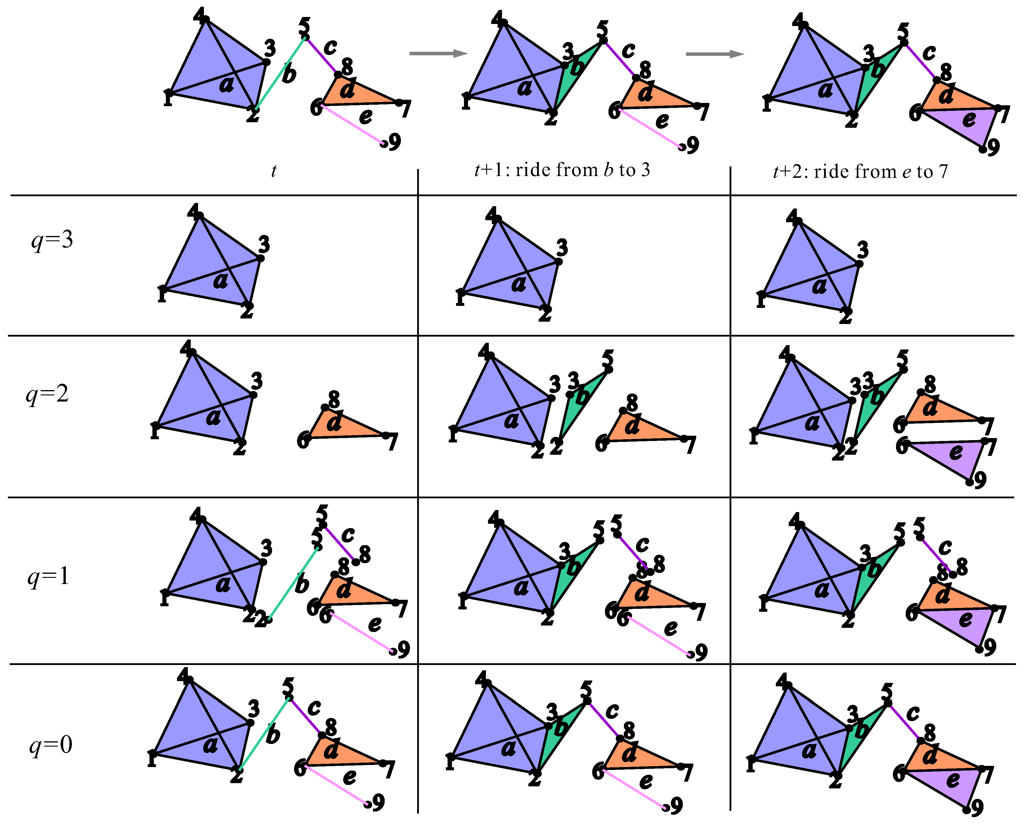
Figure 3.
An example of the embeddedness of a connected collection of simplices in simplicial complex (a) and a simplex in the connectivity class (b).
Figure 3.
An example of the embeddedness of a connected collection of simplices in simplicial complex (a) and a simplex in the connectivity class (b).

Figure 4.
Time change of the values of the entropy entries for simplicial complex of origins (a) and its conjugate complex (b).
Figure 4.
Time change of the values of the entropy entries for simplicial complex of origins (a) and its conjugate complex (b).
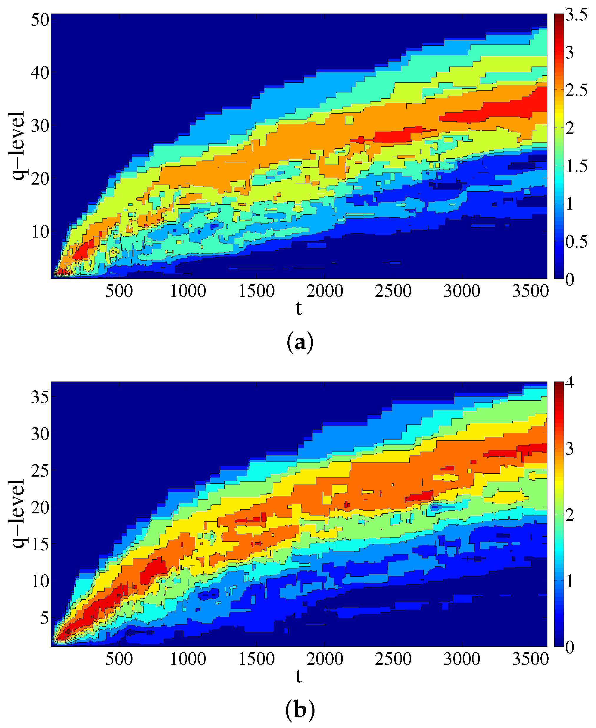
Figure 5.
Time change of the values of entropy entries for simplicial complex of origins (a) and its conjugate complex (b).
Figure 5.
Time change of the values of entropy entries for simplicial complex of origins (a) and its conjugate complex (b).
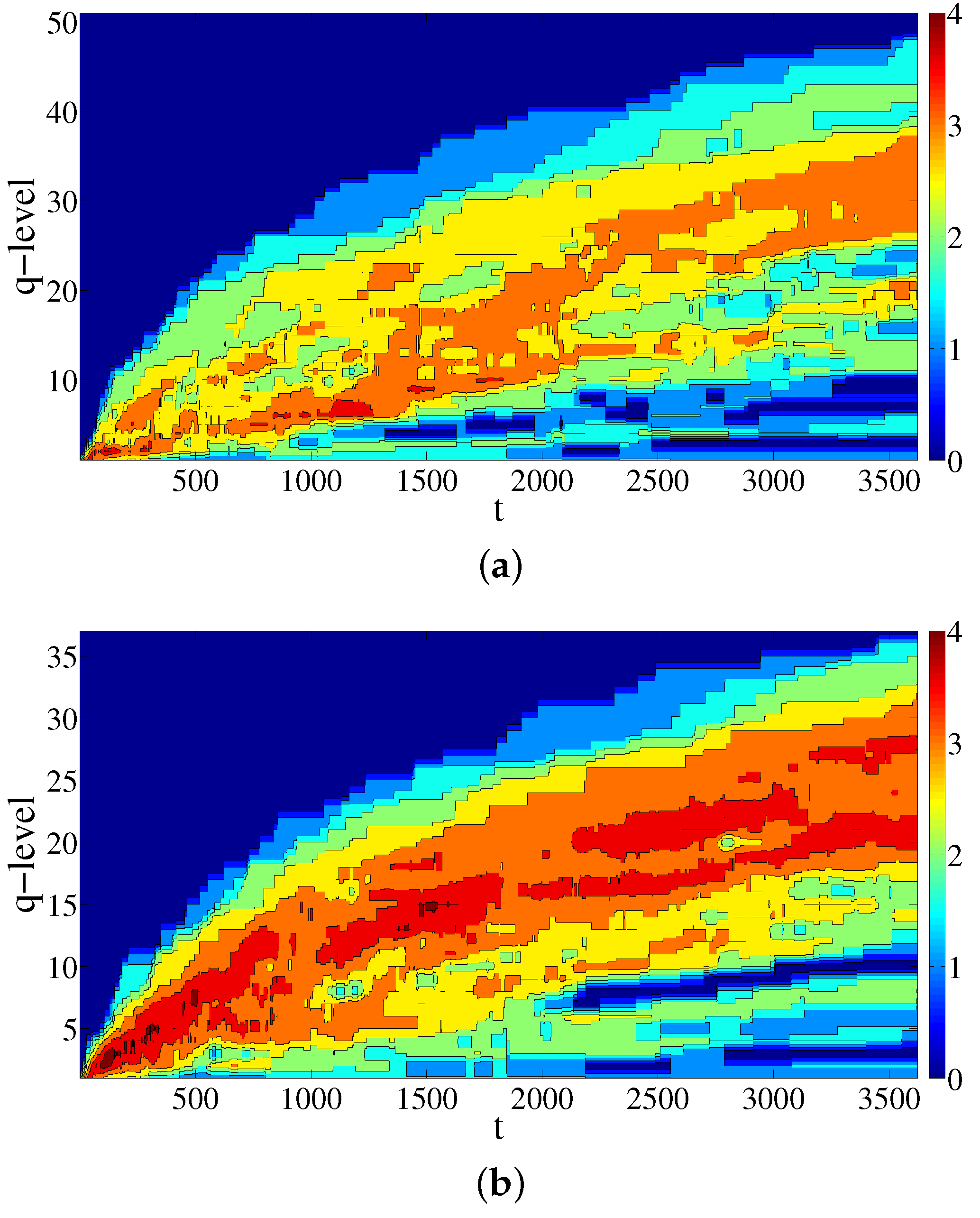
Figure 6.
Entropy structural coefficients (a–c) and (d–f) for simplicial complex and its conjugate for the original data (a,d), for the randomized destinations (b,e), and for the randomized origins (c,e) under the transition .
Figure 6.
Entropy structural coefficients (a–c) and (d–f) for simplicial complex and its conjugate for the original data (a,d), for the randomized destinations (b,e), and for the randomized origins (c,e) under the transition .

Figure 7.
Time change of the maximum values of (a) and (b) entropy entries for simplicial complex of origins and its conjugate complex of the original data.
Figure 7.
Time change of the maximum values of (a) and (b) entropy entries for simplicial complex of origins and its conjugate complex of the original data.
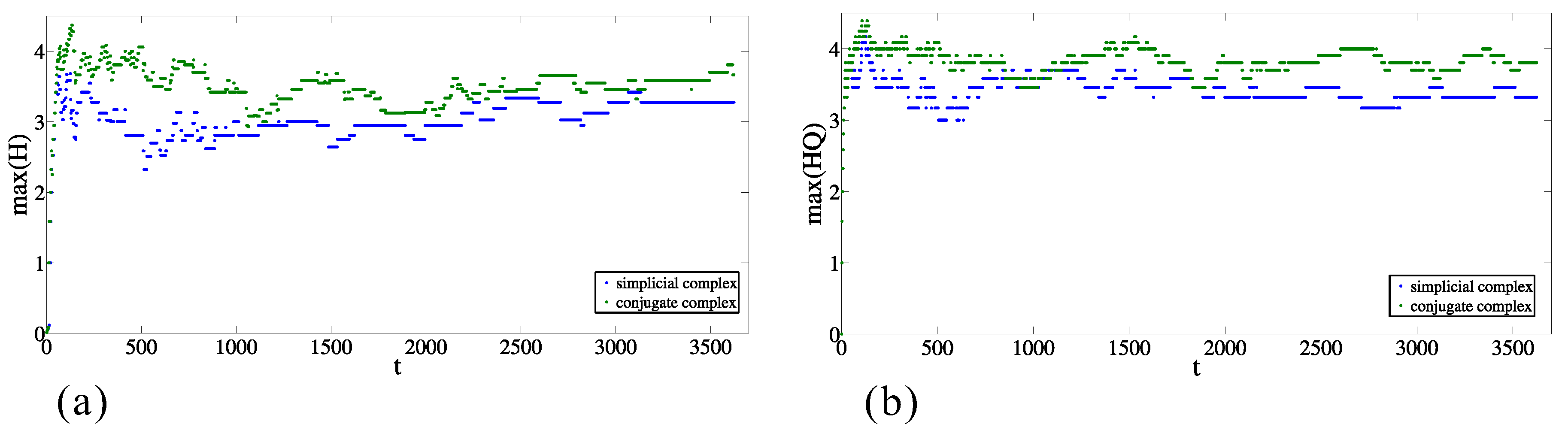
Figure 8.
Time change of the maximum values of (a) and (b) entropy entries for simplicial complex of origins and its conjugate complex for the randomized destinations.
Figure 8.
Time change of the maximum values of (a) and (b) entropy entries for simplicial complex of origins and its conjugate complex for the randomized destinations.
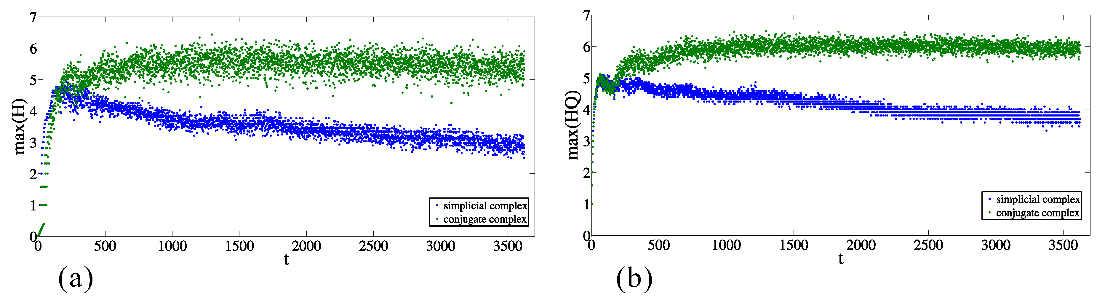
Figure 9.
Time change of the maximum values of (a) and (b) entropy entries for simplicial complex of origins and its conjugate complex for the randomized origins.
Figure 9.
Time change of the maximum values of (a) and (b) entropy entries for simplicial complex of origins and its conjugate complex for the randomized origins.

© 2017 by the authors. Licensee MDPI, Basel, Switzerland. This article is an open access article distributed under the terms and conditions of the Creative Commons Attribution (CC BY) license (http://creativecommons.org/licenses/by/4.0/).
Share and Cite
MDPI and ACS Style
Maletić, S.; Zhao, Y. Multilevel Integration Entropies: The Case of Reconstruction of Structural Quasi-Stability in Building Complex Datasets. Entropy 2017, 19, 172. https://doi.org/10.3390/e19040172
AMA Style
Maletić S, Zhao Y. Multilevel Integration Entropies: The Case of Reconstruction of Structural Quasi-Stability in Building Complex Datasets. Entropy. 2017; 19(4):172. https://doi.org/10.3390/e19040172
Chicago/Turabian StyleMaletić, Slobodan, and Yi Zhao. 2017. "Multilevel Integration Entropies: The Case of Reconstruction of Structural Quasi-Stability in Building Complex Datasets" Entropy 19, no. 4: 172. https://doi.org/10.3390/e19040172
Note that from the first issue of 2016, this journal uses article numbers instead of page numbers. See further details here.