Decomposition of the Inequality of Income Distribution by Income Types—Application for Romania


Abstract
1. Introduction
2. Problem Presentation
- To what extent is the inequality of the distribution of the total income of the population influenced by the distribution of income on the seven classes of persons. In this case, we use a decomposition of the Theil index calculated for the entire population depending on the inequality of distribution of income among the seven groups of people and the differences that exist between the seven groups. In this case, the decomposition of the Theil index corresponds to the case where the groups are disjoint [37]. The total inequality is explained by the factors that act at the level of the groups and factors that differentiate the groups of employees;
- For each group for which there are at least two income sources, the inequality of income distribution is measured by the inequality of income distribution on each source of income. In this case, because the decomposition relationship used at the previous point can no longer be used, we propose another relationship for this decomposition: the total inequality of income distributions can be decomposed into three components: the first component highlights the differences that are at the level of each data series, the second component highlights the differences between the averages of the data series, and the last term highlights the interaction between the factors.
3. Data Series
- (i)
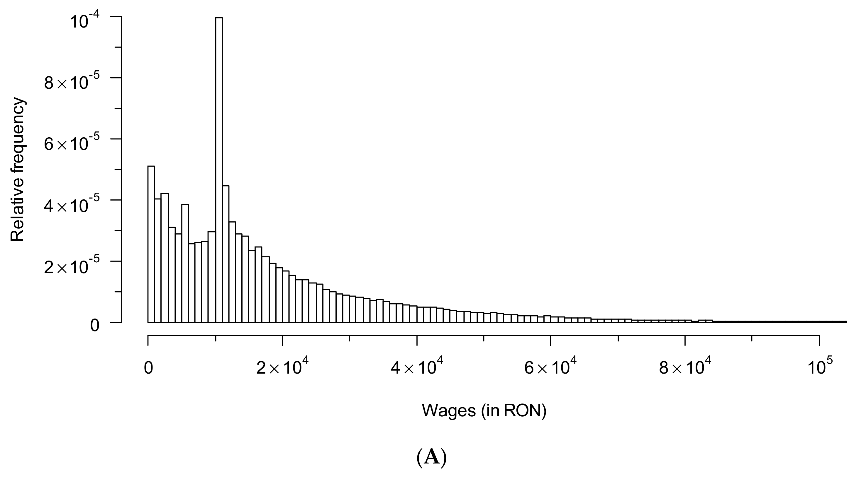
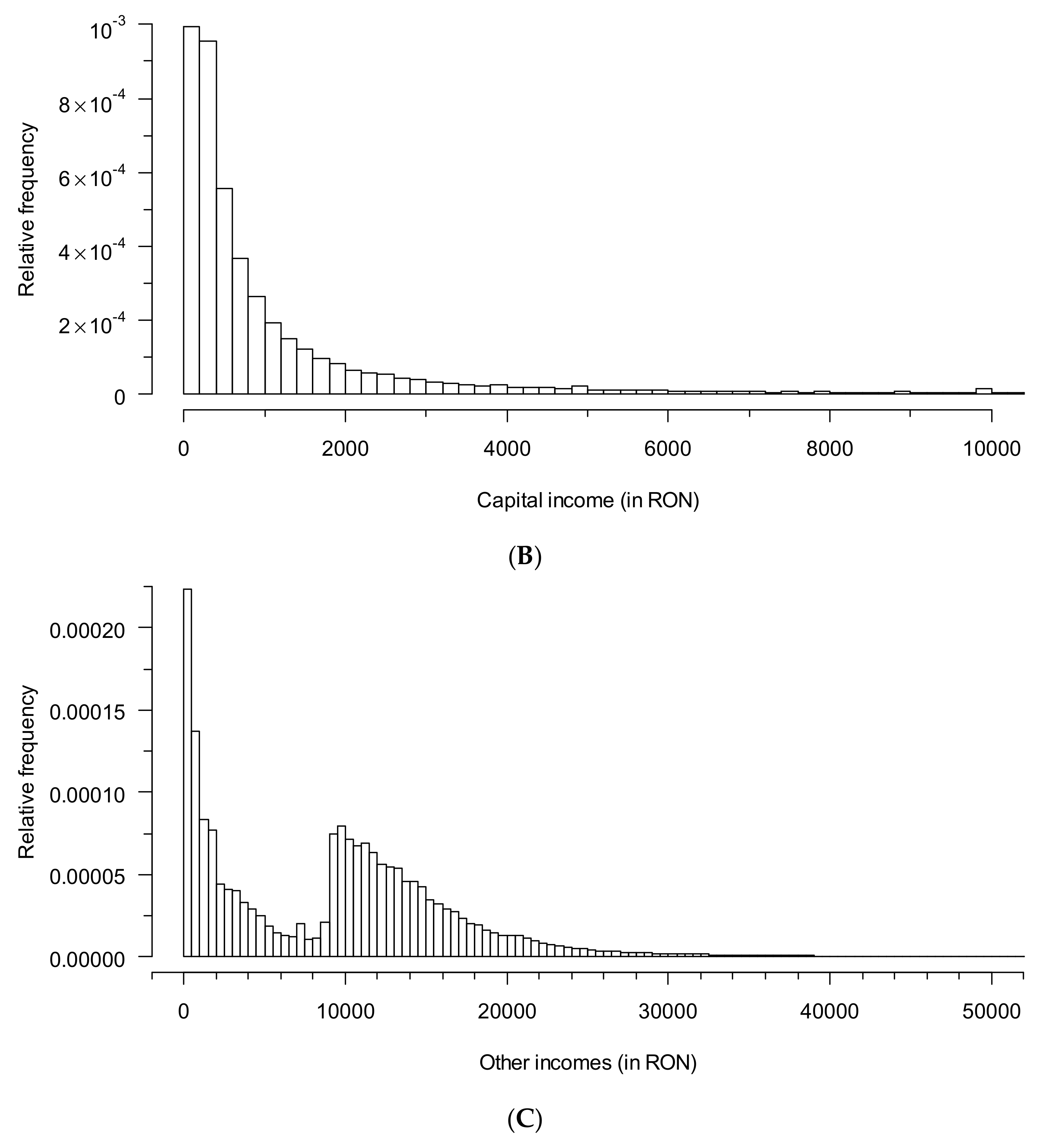
- At the level of the total population, there are significant differences in the distribution of the income obtained by the source of income (Figure 4);
- (ii)
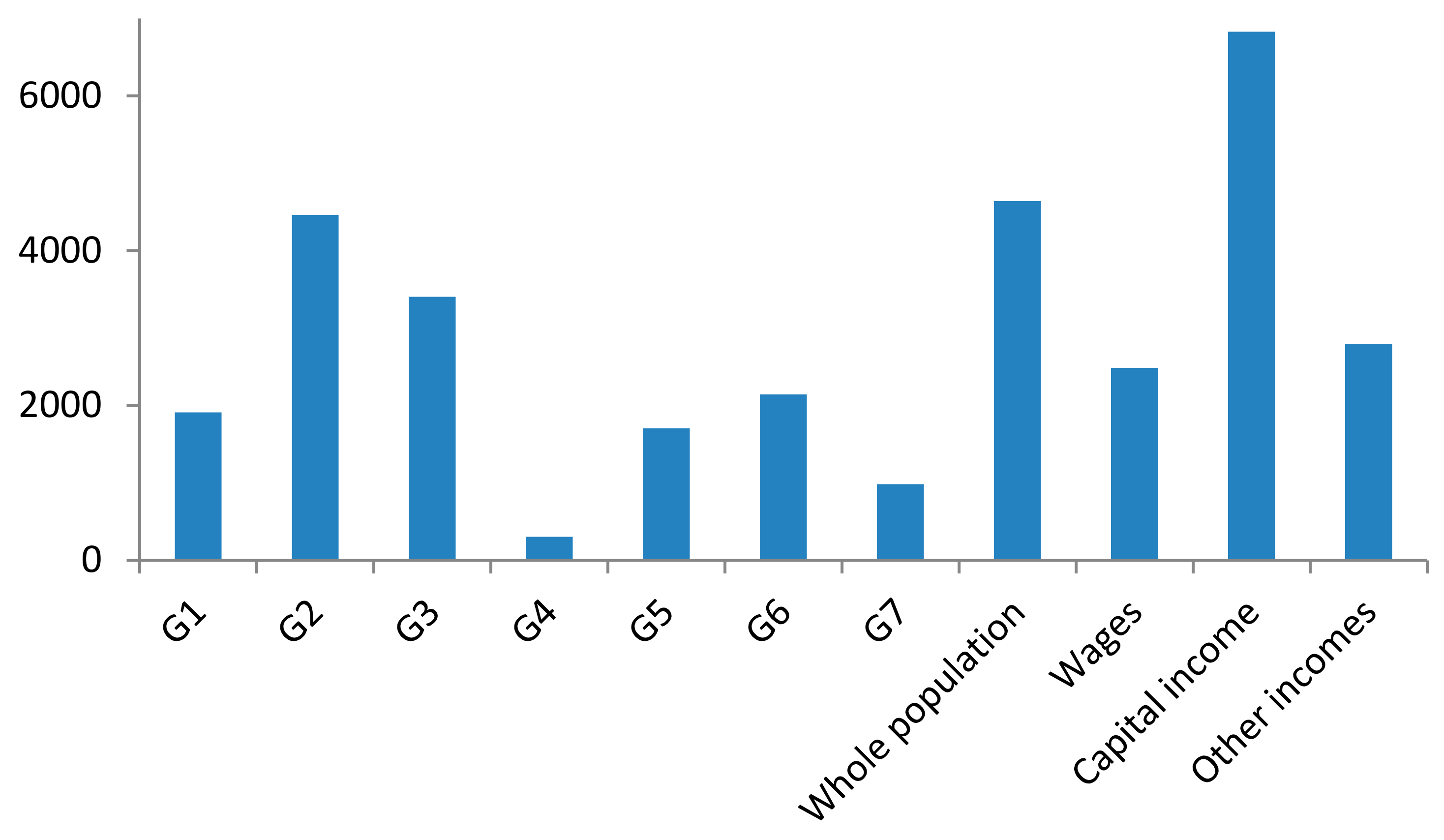
- There is a different concentration of the income from the three sources. Figure 5 shows the ratio between top 1%/bottom 99% for the total population, the seven groups, and the income from the three sources of income (we define this ratio as the ratio of the sum of incomes in the 99–100% centile to the sum of incomes in the 0–1% centile);
- (iii)
- The total income of the population is thus divided on the three sources of income: 56.0%—wages, 19.5%—capital and 24.4%—other income;
- (iv)
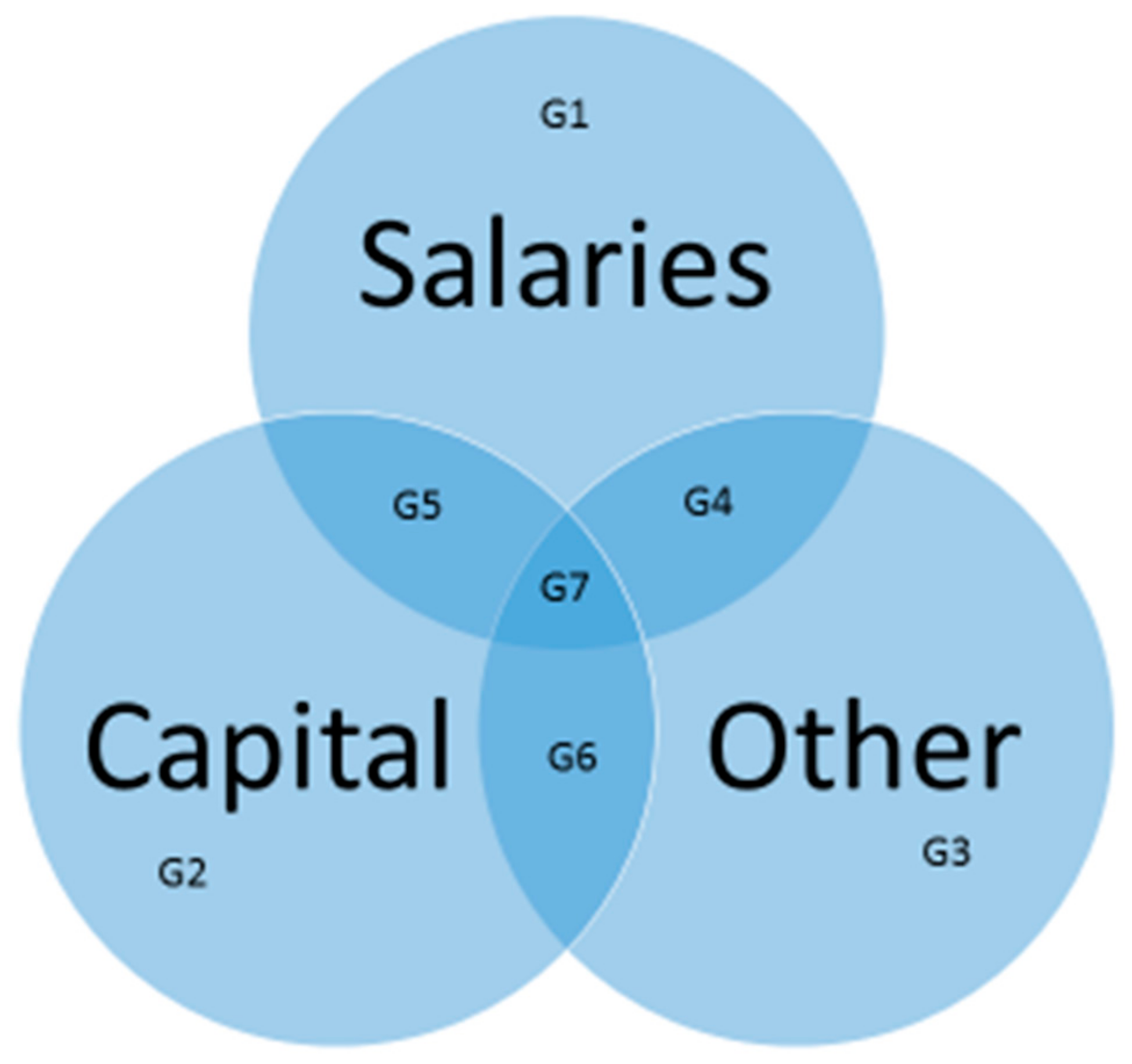
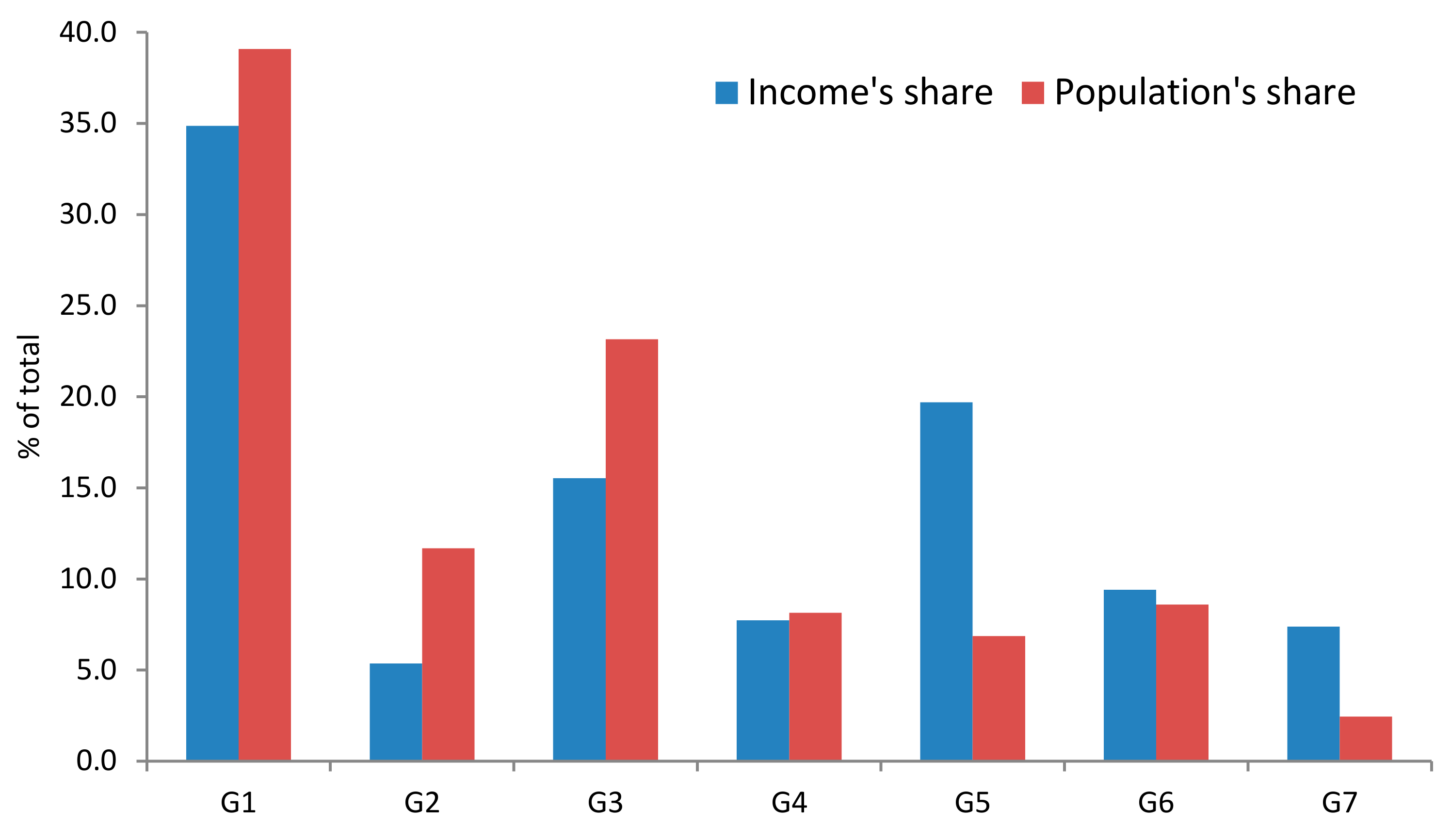
- The distribution of people who have earned income from at least one source of income on the three sources is as follows: 44% obtained at least income from wages, 23%—at least capital income and 33%—at least other income.
4. Breakdown by Disjoint Groups
- (i)
- The first term measures the inequality of income distribution as a result of the differences concerning the distribution of income in the seven groups. For each group inequality of income distribution is calculated by Theil indices and for all groups we evaluate this part of T(v) to multiply the Theil indices calculated at the group level by weighted arithmetic mean of all income;
- (ii)
- The second decomposition term in relation (3), which is denoted by , quantifies the part of the inequality of distribution of population incomes due to the differences of income distribution that exist between the seven groups. This term is a Theil index calculated for the average income at the level of the groups and using as a relative frequency the structure of the population on the seven groups from which the population is constituted.
5. Decomposing the Inequality of Income Distribution by Income Sources
- The first relationship measures the inequality of distribution of total incomes of the population due to the differences that exist in the distribution of income distributed by each income source. In this case, the Theil indices computed on the series of data constituted by income sources are multiplied by the weights of the total income from each income category in the total income of the population ;
- The second term quantifies the differences that exist between people’s income categories. This term is computed as the difference between the maximum entropy and the entropy of distributing the total income of the population by income sources ;
- The latter term is a rest that quantifies the effect of interaction between income distribution on each income category and total income distribution across the population .
6. Conclusions and Discussion
Acknowledgments
Author Contributions
Conflicts of Interest
References
- Atkinson, A.B. The Economics of Inequality; Clarendon Press: Oxford, UK, 1983; Volume 2. [Google Scholar]
- Galor, O.; Zeira, J. Income distribution and macroeconomics. Rev. Econ. Stud. 1993, 60, 35–52. [Google Scholar] [CrossRef]
- Alesina, A.; Perotti, R. Income distribution, political instability, and investment. Eur. Econ. Rev. 1996, 40, 1203–1228. [Google Scholar] [CrossRef]
- Richmond, P.; Repetowicz, P.; Hutzler, S.; Coelho, R. Comments on recent studies of the dynamics and distribution of money. Phys. A Stat. Mech. Appl. 2006, 370, 43–48. [Google Scholar] [CrossRef]
- Miśkiewicz, J. Globalization—Entropy unification through the Theil index. Phys. A Stat. Mech. Appl. 2008, 387, 6595–6604. [Google Scholar] [CrossRef]
- Miśkiewicz, J. Analysis of time series correlation. The choice of distance metrics and network structure. Acta Phys. Pol. A 2012, 121, B-89–B-94. [Google Scholar] [CrossRef]
- Dosi, G.; Fagiolo, G.; Napoletano, M.; Roventini, A. Income distribution, credit and fiscal policies in an agent-based Keynesian model. J. Econ. Dyn. Control 2013, 37, 1598–1625. [Google Scholar] [CrossRef]
- Roman, M.; Popescu, M.E. The effects of training on Romanian migrants’ income: A propensity score matching approach. J. Econ. Comput. Econ. Cybern. Stud. Res. 2015, 49, 113–128. [Google Scholar]
- Cerqueti, R.; Ausloos, M. Socio-economical analysis of Italy: The case of hagiotoponym cities. Soc. Sci. J. 2015, 52, 561–564. [Google Scholar] [CrossRef]
- Boiangiu, C.; Boiangiu, C.A.; Negrea, B.C. The entropy of transition and crisis. J. Econ. Comput. Econ. Cybern. Stud. Res. 2016, 50, 179–198. [Google Scholar]
- Taylor, L.; Rezai, A.; Foley, D.K. An integrated approach to climate change, income distribution, employment, and economic growth. Ecol. Econ. 2016, 121, 196–205. [Google Scholar] [CrossRef]
- Savage, M. Poorest Made Poorer? Decomposing Income Losses at the Bottom of the Income Distribution during the Great Recession; No. WP528; The Economic and Social Research Institute (ESRI): Dublin, Ireland, 2016. [Google Scholar]
- Berman, Y.; Ben-Jacob, E.; Shapira, Y. The dynamics of wealth inequality and the effect of income distribution. PLoS ONE 2016, 11, e0154196. [Google Scholar] [CrossRef] [PubMed]
- Dragan, I.M.; Isaic-Maniu, A. An Alternative for Indicators Which Characterize the Structure of Economic Systems. Entropy 2017, 19, 346. [Google Scholar] [CrossRef]
- Dagum, C. A new approach to the decomposition of the Gini income inequality ratio. In Income Inequality, Poverty, and Economic Welfare; Physica-Verlag HD: Heidelberg, Germany, 1998; pp. 47–63. [Google Scholar]
- Fields, G.S. Accounting for income inequality and its change: A new method, with application to the distribution of earnings in the United States. In Worker Well-Being and Public Policy; Emerald Group Publishing Limited: Bingley, UK, 2003; pp. 1–38. [Google Scholar]
- Bartolacci, F.; Castellano, N.G.; Cerqueti, R. The impact of innovation on companies’ performance: An entropy-based analysis of the STAR market segment of the Italian Stock Exchange. Technol. Anal. Strateg. Manag. 2015, 27, 102–123. [Google Scholar] [CrossRef]
- Ausloos, M.; Jovanovic, F.; Schinckus, C. On the “usual” misunderstandings between econophysics and finance: Some clarifications on modelling approaches and efficient market hypothesis. Int. Rev. Financ. Anal. 2016, 47, 7–14. [Google Scholar] [CrossRef]
- Ausloos, M.; Castellano, R.; Cerqueti, R. Regularities and discrepancies of credit default swaps: A data science approach through Benford’s law. Chaos Solitons Fractals 2016, 90, 8–17. [Google Scholar] [CrossRef]
- Bellenzier, L.; Andersen, J.V.; Rotundo, G. Contagion in the world’s stock exchanges seen as a set of coupled oscillators. Econ. Model. 2016, 59, 224–236. [Google Scholar] [CrossRef]
- Jovanovic, F.; Schinckus, C. Breaking down the barriers between econophysics and financial economics. Int. Rev. Financ. Anal. 2016, 47, 256–266. [Google Scholar] [CrossRef]
- Vitanov, N.K. Selected Models for Dynamics of Research Organizations and Research Production. In Science Dynamics and Research Production; Springer International Publishing: Cham, Switzerland, 2016; pp. 195–268. [Google Scholar]
- Vitanov, N.K. Additional Indexes and Indicators for Assessment of Research Production. In Science Dynamics and Research Production; Springer International Publishing: Cham, Switzerland, 2016; pp. 101–154. [Google Scholar]
- Varela, L.M.; Rotundo, G. Complex Network Analysis and Nonlinear Dynamics. In Complex Networks and Dynamics; Springer International Publishing: Cham, Switzerland, 2016; pp. 3–25. [Google Scholar]
- Jovanovic, F.; Schinckus, C. Econophysics and Financial Economics: An Emerging Dialogue; Oxford University Press: Oxford, UK, 2017. [Google Scholar]
- Ceptureanu, S.I.; Ceptureanu, E.G.; Orzan, M.C.; Marin, I. Toward a Romanian NPOs Sustainability Model: Determinants of Sustainability. Sustainability 2017, 9, 966. [Google Scholar] [CrossRef]
- Ausloos, M.; Bartolacci, F.; Castellano, N.G.; Cerqueti, R. Exploring how innovation strategies at time of crisis influence performance: A cluster analysis perspective. Technol. Anal. Strateg. Manag. 2017, 1–14. [Google Scholar] [CrossRef]
- Reed, W.J. The Pareto law of incomes—An explanation and an extension. Phys. A Stat. Mech. Appl. 2003, 319, 469–486. [Google Scholar] [CrossRef]
- Oancea, B.; Andrei, T.; Pirjol, D. Income distribution in Romania: The exponential-Pareto distribution. Phys. A Stat. Mech. Appl. 2017, 469, 486–498. [Google Scholar] [CrossRef]
- Tao, Y.; Wu, X.; Zhou, T.; Yan, W.; Huang, Y.; Yu, H.; Mondal, B.; Yakovenko, V.M. Universal Exponential Structure of Income Inequality: Evidence from 60 Countries. arXiv, 2016; arXiv:1612.01624. [Google Scholar]
- Derzsy, D.; Neda, Z.; Santos, M. Income distribution patterns from a complete social security database. Phys. A Stat. Mech. Appl. 2012, 391, 5611–5619. [Google Scholar] [CrossRef]
- Molnar, M. Income Distribution in Romania; Technical Report of the Institute of National Economy of the Romanian Academy; The Institute of National Economy of the Romanian Academy: București, Romania, 2010. [Google Scholar]
- Molnar, M. Income polarization in Romania. Rom. J. Econ. Forecast. 2011, 14, 64–83. [Google Scholar]
- Theil, H. Economics and Information Theory; North-Holland: Amsterdam, The Netherlands, 1967. [Google Scholar]
- Cowell, F.A. Theil, Inequality and the Structure of Income Distribution; Discussion Paper, No. DARP 67; London School of Economics & Political Science (LSE): London, UK, 2003. [Google Scholar]
- Clippe, P.; Ausloos, M. Benford’s law and Theil transform of financial data. Phys. A Stat. Mech. Appl. 2012, 391, 6556–6567. [Google Scholar] [CrossRef]
- Shorrocks, A.F. The Class of Additively Decomposable Inequality Measures. Econometrica 1980, 48, 613–625. [Google Scholar] [CrossRef]
- Cowell, F.A. Theil, Inequality Indices and Decomposition; ECINEQ WP 2005-001; Society for the Study of Economic Inequality (ECINEQ): Palma de Mallorca, Spain, 2005. [Google Scholar]
- Shorrocks, A.F. Inequality decomposition by population subgroups. Econometrica 1984, 52, 1369–1385. [Google Scholar] [CrossRef]
- Toyoda, T. Decomposability of inequality measures. Econ. Stud. Q. 1980, 31, 207–246. [Google Scholar]
- Foster, J.E.; Shneyerov, A.A. A general class of additively decomposable inequality measures. Econ. Theory 1999, 14, 89–111. [Google Scholar] [CrossRef]
- Bourguignon, F. Decomposable income inequality measures. Econometrica 1979, 47, 901–920. [Google Scholar] [CrossRef]
- Fields, G.S. Measuring Inequality Change in an Economy with Income Growth. In Economics: Income Distribution; The International Library of Critical Writings in Economics Series; Edward Elgar: Cheltenham, UK, 2000. [Google Scholar]
- Morduch, J.; Sicular, T. Rethinking inequality decomposition, with evidence from rural China. Econ. J. 2002, 112, 93–106. [Google Scholar] [CrossRef]
- Derrick, B.; Dobson-Mckittrick, A.; Toher, D.; White, P. Test statistics for comparing two proportions with partially overlapping samples. J. Appl. Quant. Methods 2015, 10, 1–14. [Google Scholar]
- Furtună, T.F.; Vinţe, C. Integrating R and Java for Enhancing Interactivity of Algorithmic Data Analysis Software Solutions. Rom. Stat. Rev. 2016, 64, 29–41. [Google Scholar]
- Seljak, R.; Pikelj, J. Statistical Data Processing with R–Metadata Driven Approach. Rom. Stat. Rev. 2016, 64, 71–78. [Google Scholar]
- Tsallis, C. Possible generalization of Boltzmann–Gibbs statistics. J. Stat. Phys. 1988, 52, 479–487. [Google Scholar] [CrossRef]
- Ausloos, M.; Miśkiewicz, J. Introducing the q-Theil index. Braz. J. Phys. 2009, 39, 388–395. [Google Scholar]


| Whole Population (Wages) | Whole Population (Capital Income) | Whole Population (Other Incomes) | Whole Population (Total Income) | |
|---|---|---|---|---|
| Average | 20,623.12 | 13,752.05 | 12,017.18 | 20,826.43 |
| Standard deviation | 33,360.71 | 1,730,903 | 49,355.52 | 942,825.90 |
| Median | 12,400 | 598 | 9960 | 11,348 |
| Coefficient of variance (%) | 161.76 | 12,586.51 | 410.71 | 4527.07 |
| Top 10%/bottom 90% | 78.91 | 1005.03 | 208.40 | 387.27 |
| Top 1%/bottom 99% | 2487.23 | 6827.21 | 2795.66 | 4640.43 |
| Mean/Median | 1.66 | 23.00 | 1.21 | 1.84 |
| G1 (wages) | G2 (capital income) | G3 (other incomes) | ||
| Average | 18,574.47 | 9562.41 | 13,971.92 | For G1, G2 and G3 the results for “Total income” are identical with those on different income source |
| Standard deviation | 26,229.85 | 1149,281 | 60,275.29 | |
| Median | 12,035 | 470 | 10,428 | |
| Coefficient of variance | 1.41 | 12,018.75 | 431.40 | |
| Top 10%/bottom 90% | 65.94 | 713.38 | 183.14 | |
| Top 1%/bottom 99% | 1912.47 | 4460.42 | 3403.67 | |
| Mean/Median | 1.54 | 20.35 | 1.34 | |
| G4 (wages and other incomes) | ||||
| Average | 14,759.89 | Not the case | 5009.29 | 19,769.19 |
| Standard deviation | 20,776.91 | 13,612.08 | 26,077.56 | |
| Median | 9843 | 1611 | 13,203 | |
| Coefficient of variance | 140.77 | 271.74 | 131.91 | |
| Top 10%/bottom 90% | 88.06 | 169.03 | 27.48 | |
| Top 1%/bottom 99% | 2182.35 | 1358.48 | 305.33 | |
| Mean/Median | 1.50 | 3.11 | 1.50 | |
| G5 (wages and capital income) | ||||
| Average | 37,104.79 | 22,572.58 | Not the case | 59,677.37 |
| Standard deviation | 59,334.21 | 468,643.80 | 473,716.70 | |
| Median | 21,979 | 703 | 27,973 | |
| Coefficient of variance | 159.91 | 2076.16 | 793.80 | |
| Top 10%/bottom 90% | 54.45 | 1635.26 | 69.82 | |
| Top 1%/bottom 99% | 1564.80 | 10,661.56 | 1705.22 | |
| Mean/Median | 1.69 | 32.11 | 2.14 | |
| G6 (capital and other sources of income) | ||||
| Average | Not the case | 9198.97 | 13,612.48 | 22,811.45 |
| Standard deviation | 1,816,826 | 38,784.26 | 1,817,392 | |
| Median | 666 | 12,501 | 14,049 | |
| Coefficient of variance | 19,750.32 | 284.92 | 7967.02 | |
| Top 10%/bottom 90% | 629.44 | 78.26 | 98.62 | |
| Top 1%/bottom 99% | 4897.98 | 1046.05 | 2142.05 | |
| Mean/Median | 13.81 | 1.09 | 1.62 | |
| G7 (wages, capital and other incomes) | ||||
| Average | 26,545.61 | 24,924.32 | 11,244.93 | 62,714.87 |
| Standard deviation | 49,203.57 | 4,204,152 | 40,777.57 | 4,204,975 |
| Median | 14,400 | 825 | 4270.5 | 28,573.50 |
| Coefficient of variance | 185.35 | 16,867.67 | 362.63 | 6704.91 |
| Top 10%/bottom 90% | 104.36 | 1774.50 | 1328.07 | 54.01 |
| Top 1%/bottom 99% | 2975.03 | 13,926.05 | 1509.16 | 982.31 |
| Mean/Median | 1.84 | 30.21 | 2.63 | 2.19 |
| Population | G1 | G2 | G3 | G4 | G5 | G6 | G7 | Whole Population |
|---|---|---|---|---|---|---|---|---|
| Theil Index | 0.47 | 3.73 | 0.88 | 0.42 | 1.06 | 1.56 | 1.95 | 1.18 |
| Theil Index | Share (%) of the Inequality Measured by the Theil Index of Each Group | |
|---|---|---|
| G1 | 0.47 | 13.91 |
| G2 | 3.73 | 16.89 |
| G3 | 0.88 | 11.52 |
| G4 | 0.42 | 2.71 |
| G5 | 1.06 | 17.66 |
| G6 | 1.56 | 12.44 |
| G7 | 1.95 | 12.21 |
| Whole population | 1.18 | 100 |
| Within groups | 1.03 | 87.34 |
| Between groups | 0.15 | 12.66 |
| Theil Index | Contribution to Total Inequality (%) | |
|---|---|---|
| G4: Wages | 0.53 | - |
| Other incomes | 0.97 | - |
| Whole population | 0.42 | 100.0 |
| 0.64 | 154.3 | |
| 0.13 | 30.6 | |
| −0.35 | −84.9 | |
| G5: Wages | 0.56 | - |
| Capital income | 3.12 | - |
| Whole population | 1.06 | 100.0 |
| 1.53 | 144.0 | |
| 0.03 | 2.8 | |
| −0.50 | −46.8 | |
| G6: Other incomes | 0.34 | - |
| Capital income | 4.43 | - |
| Whole population | 1.56 | 100.0 |
| 1.99 | 127.3 | |
| 0.02 | 1.2 | |
| −0.45 | −25.8 | |
| G7: Wages | 0.66 | - |
| Capital income | 5.29 | - |
| Other incomes | 1.00 | - |
| Whole population | 1.95 | 100.0 |
| 2.56 | 131.0 | |
| 0.06 | 3.1 | |
| −0.67 | −34.1 |
© 2017 by the authors. Licensee MDPI, Basel, Switzerland. This article is an open access article distributed under the terms and conditions of the Creative Commons Attribution (CC BY) license (http://creativecommons.org/licenses/by/4.0/).
Share and Cite
Andrei, T.; Oancea, B.; Richmond, P.; Dhesi, G.; Herteliu, C. Decomposition of the Inequality of Income Distribution by Income Types—Application for Romania. Entropy 2017, 19, 430. https://doi.org/10.3390/e19090430
Andrei T, Oancea B, Richmond P, Dhesi G, Herteliu C. Decomposition of the Inequality of Income Distribution by Income Types—Application for Romania. Entropy. 2017; 19(9):430. https://doi.org/10.3390/e19090430
Chicago/Turabian StyleAndrei, Tudorel, Bogdan Oancea, Peter Richmond, Gurjeet Dhesi, and Claudiu Herteliu. 2017. "Decomposition of the Inequality of Income Distribution by Income Types—Application for Romania" Entropy 19, no. 9: 430. https://doi.org/10.3390/e19090430
APA StyleAndrei, T., Oancea, B., Richmond, P., Dhesi, G., & Herteliu, C. (2017). Decomposition of the Inequality of Income Distribution by Income Types—Application for Romania. Entropy, 19(9), 430. https://doi.org/10.3390/e19090430