Partial Discharge Feature Extraction Based on Ensemble Empirical Mode Decomposition and Sample Entropy

Abstract

Partial Discharge (PD) pattern recognition plays an important part in electrical equipment fault diagnosis and maintenance. Feature extraction could greatly affect recognition results. Traditional PD feature extraction methods suffer from high-dimension calculation and signal attenuation. In this study, a novel feature extraction method based on Ensemble Empirical Mode Decomposition (EEMD) and Sample Entropy (SamEn) is proposed. In order to reduce the influence of noise, a wavelet method is applied to PD de-noising. Noise Rejection Ratio (NRR) and Mean Square Error (MSE) are adopted as the de-noising indexes. With EEMD, the de-noised signal is decomposed into a finite number of Intrinsic Mode Functions (IMFs). The IMFs, which contain the dominant information of PD, are selected using a correlation coefficient method. From that, the SamEn of selected IMFs are extracted as PD features. Finally, a Relevance Vector Machine (RVM) is utilized for pattern recognition using the features extracted. Experimental results demonstrate that the proposed method combines excellent properties of both EEMD and SamEn. The recognition results are encouraging with satisfactory accuracy.

1. Introduction

Partial discharge (PD) detection plays an important role in the evaluation of insulation condition [1]. Different PD types may cause diverse damages to equipment insulation [2]. Therefore, it is meaningful to be able to distinguish between different PD types for electrical equipment repair and maintenance [3,4].

Feature extraction is of great importance during PD pattern recognition. It directly affects the recognition results [5,6,7,8,9]. Chu et al. employed statistical distribution parameters method for PD recognition. Different types of PD have been identified [5]. Ma et al. used the fractal theory for motor single-source PD classification [6]. Cui et al. adopted the image moments characteristic parameter of PD to analyze the surface discharge development process [7]. However, the data size of these methods is very large and the speed of data processing is slow, which is not suitable for online monitoring. Alvarez et al. extracted the waveform feature parameters to discriminate the PD sources [8]. However, the electromagnetic wave radiated by the PD pulse will decay and can be negatively influenced by the electromagnetic interference. Tang et al. used wavelet decomposition method for PD recognition in gas-insulated switchgear (GIS) [9]. However, his method has some inherent limitation, such as the difficulty of the selection of wavelet basis, wavelet thresholds, decomposition levels, and so on.

Empirical Mode Decomposition (EMD), proposed by Huang et al. in 1998, is a self-adapting method for signal decomposition [10]. It is a data-driven approach that is suitable for analyzing non-linear and non-stationary problems. However, it is restricted by its inherent mode-mixing phenomenon. Boudraa et al. put forward a signal filtering method based on EMD [11]. It is limited to signals that were corrupted by additive white Gaussian noise. To solve the mode-mixing problem in EMD, Ensemble Empirical Mode Decomposition (EEMD) was proposed by Wu and Huang [12]. White noise components are added artificially in EEMD and eliminated through repetitive averaging. EEMD decomposes signals into Intrinsic Mode Functions (IMFs) containing signals’ local features. It could effectively apply the uniform distribution character to make up for the absence of signal scales. It is also suitable for non-linear and non-stationary signals. Furthermore, EEMD has been widely adopted in fault feature extraction [13,14,15,16]. Fu et al. proposed a novel approach based on fast EEMD to extract the fault feature of bearing vibration signals [13]. The test results from both the simulation signal and the experiment data demonstrated its effectiveness. The heart phonocardiogram is analyzed in [14] by employing EEMD combined with kurtosis features. Its practicality was proven through the experimental dataset obtained from 43 heart sound recordings in a real clinical environment. Kong et al. proposed an envelope extraction method based on EEMD for the double-impulse extraction of faulty hybrid ceramic ball bearings [15]. The pre-whitened signals were de-noised using EEMD, and the Hilbert Envelope Extraction Method was employed to extract the double impulse. Simulation results verified the validity of this method. Patel et al. presented a novel approach by combining template matching with EEMD [16]. EEMD was applied to decompose the noisy data into IMFs. However, the data size of IMFs is always large. To reduce the calculation, some steps should be taken to extract the IMFs that represent prominent features.

Sample Entropy (SamEn) is the negative natural logarithm of the conditional probability [17]. A lower SamEn value indicates more self-similarity in a time series. SamEn has many positive characteristics, such as good residence to noise interference and closer agreement between theory for data sets and known probabilistic content. Widodo et al. presented the intelligent prognostics for battery health based on sample entropy [18]. SamEn features could represent the health condition of battery. Mei et al. used sample entropy to quantify parameters of four foot types. From this, it could be used to quantify the regularity and complexity of a data series [19]. SamEn could avoid the influence of the noise when exploring a time series. Therefore, SamEn is an effective tool for evaluating complex non-linear time series. Moreover, SamEn displays the property of relative consistency in situations where approximate entropy does not. In practice these characteristics are suitable for PD signal analysis. In this study SamEn is adopted to extract the representative characteristics from IMFs of EEMD.

In recent years, various pattern recognition approaches have been used in PD pattern recognition [20,21]. Majidi et al. created seventeen samples for classifying internal, surface, and corona partial discharges in the laboratory [20]. Different PD types were identified with an artificial neural network (ANN) and the sparse method. However, an ANN presents problems of slow convergence rate and the tendency to be entrapped in a local minimum. As a learning machine, which is based on kernel functions, a Support Vector Machine (SVM) classifier could effectively solve such problems. In Reference [21], the PD and noise-related coefficients are identified by SVM. The performance was evaluated with PD signals measured in air and in solid dielectrics. However, SVM is restricted in practical applications for its inherent restriction by Mercer conditions and the difficult choice of regularization parameters [22].

Relevance Vector Machine (RVM), proposed by Tipping, is a novel pattern recognition method based on kernel functions [23]. The model is learning under a Bayesian framework, whose kernel functions are not restricted by Mercer conditions. Moreover, the regularization coefficient is adjusted automatically during the estimation of hyper parameters. As an extension of SVM, RVM has become the research focus in recent years [24,25,26]. Nguyen employed RVM for Kinect gesture recognition and compared it with SVM [24]. Results showed that RVM could achieve the state-of-the-art predictive performance and run much faster than SVM. Compared with SVM, RVM needs fewer vectors, and could effectively avoid the choice of regularization coefficient and restriction of Mercer conditions. Liu et al. proposed an intelligent multi-sensor data fusion method using RVM for gearbox fault detection [25]. Experimental results demonstrated that RVM not only has higher detection accuracy, but also has better real-time accuracy. It has been shown in literature that RVM can be very sensitive to outliers far from the decision boundary that discriminates between two classes. To solve this problem, Hwang proposed a robust RVM based on a weighting scheme that is insensitive to outliers [26]. Experimental results from synthetic and real data sets verified its effectiveness. In this paper, RVM is used to recognize the different PD types using extracted features. The resulting recognition achieved encouraging accuracy.

The rest of this paper is organized as follows: Section 2 introduces the conception of EMD, EEMD, Sample Entropy and RVM, and also presents the feature extraction approach based on EEMD-SamEn. Section 3 describes the PD experiments and calculates the PD parameters. Section 4 evaluates the performance of the proposed method and compares it with different feature extraction methods. Finally, Section 5 concludes this paper.

2. Feature Extraction Based on Ensemble Empirical Mode Decomposition and Sample Entropy

2.1. Review of Empirical Mode Decomposition

Empirical Mode Decomposition (EMD), proposed by Huang et al., is a novel self-adapting method especially for non-linear analysis and processing non-stationary signals. With EMD, one signal can be decomposed into some IMFs and a residual. EMD has been widely used in the area of signal analysis and processing [10,11]. However, it is restricted by its inherent mode-mixing problem in practical applications.

2.2. Review of Enseble Empirical Mode Decomposition

Ensemble Empirical Mode Decomposition (EEMD) is proposed by Wu and Huang, and is aimed at eliminating the mode-mixing in EMD. EEMD represents an extension of EMD [12]. The algorithm procedure can be shortly defined in the following steps:

(1)

Add a generated white noise $s(t)$ to the original signal x₀(t):

X(t) = x₀(t) + s(t)

(1)

(2)

Decompose $X(t)$ into IMFs c_j(t) and a residual r_n(t).

$$X(t)={\displaystyle \sum _{j=1}^n{c}_j(t)+r_n(t)}$$

(2)

(3)

Add different white noise $s_i(t)$ to the original signal. Repeat (1) and (2).

$$X_i(t)={\displaystyle \sum _{j=1}^n{c}_i{}_j(t)+r_{in}(t)}$$

(3)

(4)

Calculate the IMFs component $c_n(t)$ corresponding to the original signal where:

$$c_n(t)=\frac{1}{N_s}{\displaystyle \sum _{i=1}^{N_s}{c}_{i,n}(t)}$$

(4)

The white noise number added in EEMD conforms to the statistical law:

$${\epsilon }_n=\frac{\epsilon }{\sqrt{N_s}}$$

(5)

where $N_s$ is the added number of white noise, $\epsilon$ is the noise amplitude, ${\epsilon }_n$ is the error caused by the superposition of original signals and the final IMFs.

(5)

The final signal, x(t), can be decomposed as the following time series:

$$x(t)={\displaystyle \sum _{n=1}^{N_s}{c}_n(t)+r_n(t)}$$

(6)

2.3. Sample Entropy

Sample Entropy (SamEn), proposed by Richman, was used to evaluate the complexity of a time series. The procedure can be expressed as follows:

(1)

Construct a m-dimension vector with time series v(t).

(2)

Define the distance between m-dimension vectors V(i) and V(j) as:

$$d[V(i),V(j)]=\underset{k=0\cdots ,m-1}{\max }[\left|v(i+k)-v(j+k)\right|]$$

(7)

(3)

Given a threshold, r, calculate the ratio $B_{{}_i}^m(r)$ between the number of $d[V(i),V(j)]<r$ and N − m − 1:

$$B_{{}_i}^m(r)=\frac{1}{N-m-1}\{d[V(i),V(j)]<r\}$$

(8)

where $i=1,2,\cdots ,N-m+1$, $i\ne j$.

(4)

The mean value of $B_{{}_i}^m(r)$ is defined as:

$${\overline{B}}^m(r)=\frac{1}{N-m-1}{\displaystyle \sum _{i=1}^{N-m+1}{B}_{{}^i}^m(r)}$$

(9)

(5)

As for m + 1, ${\overline{B}}^{m+1}(r)$ can be obtained using Steps (1)–(4).

(6)

The SamEn of the given time series v(t) can be defined as:

$$\mathrm{SamEn}(m,r)=\underset{N\to \infty }{\lim }[-\ln \frac{{\overline{B}}^{m+1}(r)}{{\overline{B}}^m(r)}]$$

(10)

where N is a finite value, then SamEn can be expressed as:

$$\mathrm{SamEn}(m,r,N)=-\ln \frac{{\overline{B}}^{m+1}(r)}{{\overline{B}}^m(r)}$$

(11)

2.4. Relevance Vector Machine (RVM)

Given input training datasets $D_i={\{d_i,t_i\}}_{i=1}^N$, where $d_i$ is the input vector, $t_i$ is the output vector. RVM output model can be defined as:

$$y(d_i)={\displaystyle \sum _{i=1}^N{w}_i{\varphi }_i(d_i)}$$

(12)

where $w_i$ is the weight vector, ${\varphi }_i(d)$ is a non-linear basis function. The likelihood of the whole dataset can be defined as:

$$P(t|w)={\displaystyle \prod _{i=1}^N\sigma {\{y(d_i;w)\}}^{t_i}{[1-\sigma \{y(d_i;w)\}]}^{1-t_i}}$$

(13)

in which $t=(t_1,\cdots ,t_n)$, $w=(w_0,\cdots ,w_n)$, $\sigma (\cdot )$ is a Sigmoid function.

Gaussian prior probability distribution is defined as:

$$p(w|\alpha )={\displaystyle \prod _{i=0}^{N}N(w_i|0,{\alpha }_i^{-1}})$$

(14)

where $\alpha ={({\alpha }_0,{\alpha }_1,\cdots ,{\alpha }_N)}^{\mathrm{T}}$ is the hyper-parameter of the prior probability distribution. For the new input vector $d_{*}$, the probability prediction of the target value $t_{*}$ can be described as:

$$p(t_{*}|t)={\displaystyle \int p(t_{*}|w,\alpha )p(w|t,\alpha })p(\alpha |t)\mathrm{d}w\mathrm{d}\alpha$$

(15)

For the fixed value of $\alpha$, the maximum posterior probability estimation concerning w can be equated with the calculation of the maximum of Equation (16).

$$\log \{p(t|w)p(w|\alpha )\}={\displaystyle \sum _{i=1}^N[t_i\log y_i+(1-t_i)\log (1-y_i)]}-\frac{1}{2}{w}^{\mathrm{T}}Aw$$

(16)

where $A=\mathrm{diag}({\alpha }_0,{\alpha }_1,\cdots ,{\alpha }_N)$, $y_i=\sigma \{y(d_i;w)\}$.

The Hessian matrix at W_MP can be defined as:

$${\nabla }_{\mathrm{w}}{\nabla }_{\mathrm{w}}\log p(w|t,\alpha ){|}_{w_{\mathrm{MP}}}=-({\varphi }^{\mathrm{T}}B\varphi +A)$$

(17)

where $B=\mathrm{diag}({\beta }_1,{\beta }_2,\cdots ,{\beta }_N)$, ${\beta }_i=y_i(1-y_i)$.

Based on Equation (17), the covariance matrix of the posterior probability at $w_{\mathrm{MP}}$ can be obtained as:

$${\displaystyle \sum ={({\varphi }^{\mathrm{T}}B\varphi +A)}^{-1}}$$

(18)

$w_{\mathrm{MP}}$ can be defined as:

$$w_{\mathrm{MP}}={\displaystyle \sum {\varphi }^{\mathrm{T}}Bt}$$

(19)

The hyper-parameter $\alpha$ can be updated with MacKay [27]:

$${\alpha }_i^{new}=\frac{{\gamma }_i}{w_{{\mathrm{MP}}_i}^2},{\gamma }_i=1-{\alpha }_i{\displaystyle \sum i,i}$$

(20)

where $w_{{\mathrm{MP}}_i}$ is the i-th element of the posterior probability weight from Equation (19), ${\displaystyle \sum i,i}$ is the i-th diagonal element of the posterior weight covariance from Equation (18).

After obtaining ${\alpha }^{new}$, the mean of posterior probability is re-estimated and the covariance matrix is re-calculated. An iterative process of Equations (18)–(20) is repeated until proper convergence criteria are satisfied. After iterations, the sample vectors concerning the basic functions of non-zero weights are the Relevance Vectors (RV).

2.5. Feature Extraction Based on Enseble Empirical Mode Decomposition and Sample Entropy

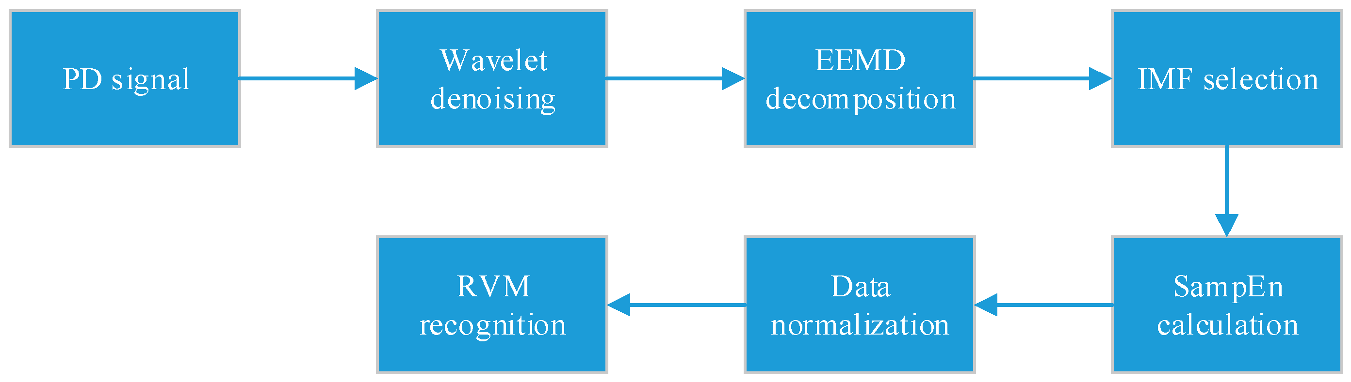
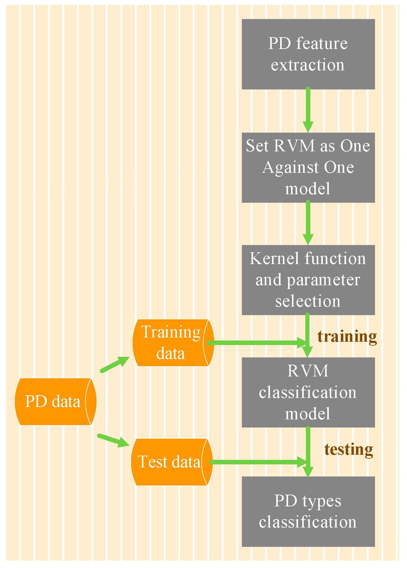
The proposed method adopts wavelet method for de-noising of the original PD signals. Next, IMF components are extracted by EEMD of the de-noised signals. After that, the correlation coefficient method is applied to IMF selection and is followed by calculating the SamEn of each IMF. Finally, RVM is employed for PD pattern recognition with the extracted characteristic values. The feature extraction steps are as follows:

(1)

Extract different types of PD signals under different voltage levels in the laboratory environment.

(2)

Process the original PD signal with wavelet method to eliminate background interferences.

(3)

Decompose de-noised signals with EEMD and obtain a set of IMFs.

(4)

Calculate the correlation coefficient, C, of each IMF component with Equation (21).

$$C=\frac{{\displaystyle \sum _{i=1}^n(r_i-\overline{r})(x_i-\overline{x})}}{\sqrt{{\displaystyle \sum _{i=1}^n{(r_i-\overline{r})}^2}}\sqrt{{\displaystyle \sum _{i=1}^n{(x_i-\overline{x})}^2}}}$$

(21)

where C is the correlation coefficient between IMFs and the signal, r is the IMF, x represents the original PD signal, and n is the number of IMFs. The larger the value of $\left|C\right|$, the greater the relevance between r and x. If the correlation coefficient C is close to 0, then the linear correlation relationship between r and x is very weak.

(5)

Select those IMFs that have a large value of $\left|C\right|$.

(6)

Calculate the sample entropy of each extracted IMF.

(7)

Load sample entropy vectors into the RVM classifier and obtain the recognition results.

The flow diagram of PD feature extraction based on the proposed method is shown in Figure 1.

3. Experiment and Analysis

3.1. Signal Extraction

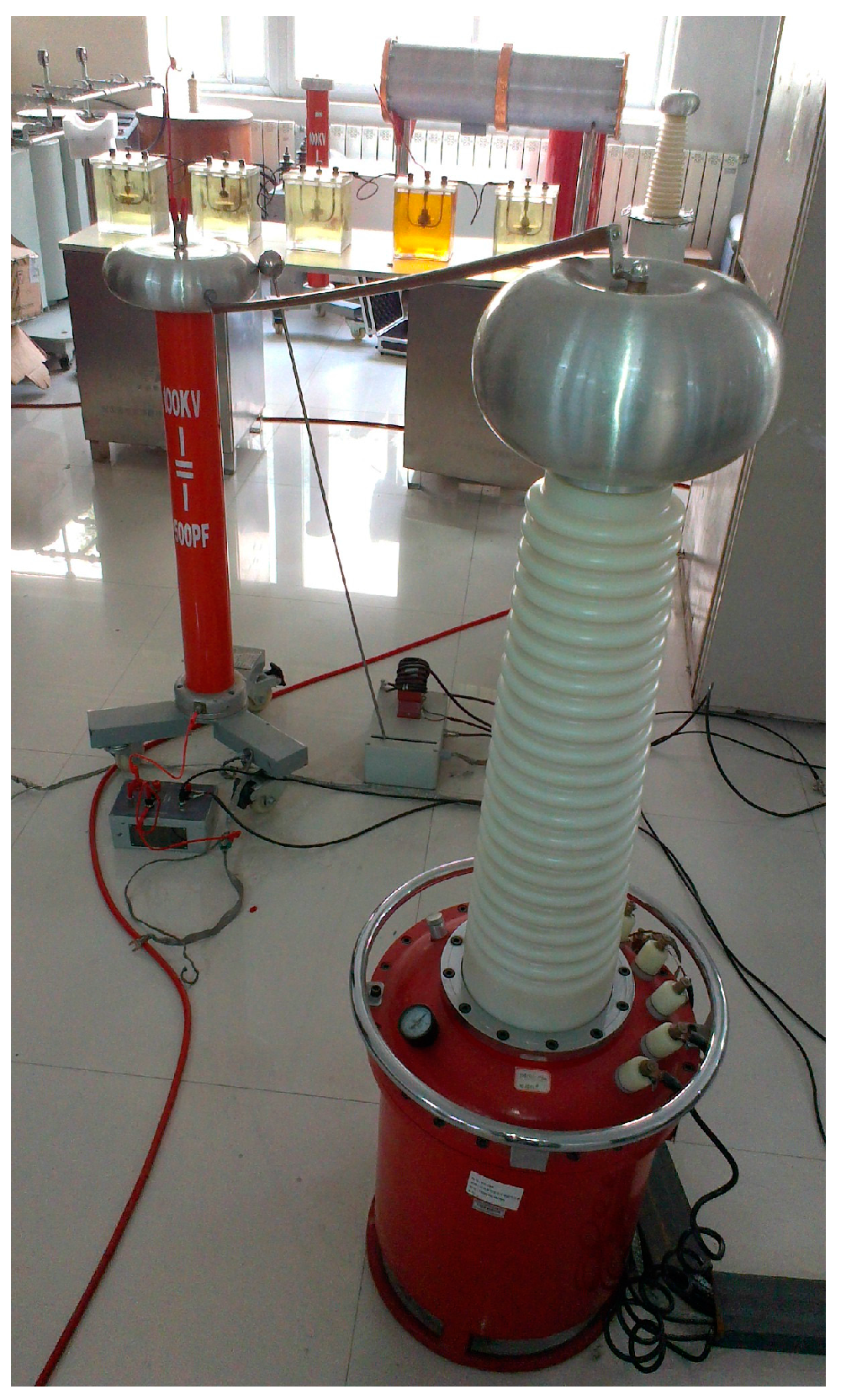
Different PD types can produce different effects in insulation materials, but the range can be diverse. To analyze the characteristics of different PD types, PD signals of different models are extracted in the laboratory. According to the inner insulation structure of power transformers [28,29], there are four possible different PD types, including floating discharge (FD), needle-plate discharge (ND), surface discharge (SD), and air-gap discharge (AD). PD models are shown in Figure 2. The experimental setup is shown in Figure 3. All the models are placed in the fuel tank filled with transformer oil. The PD signal is detected in the simulated transformer tank in the laboratory.

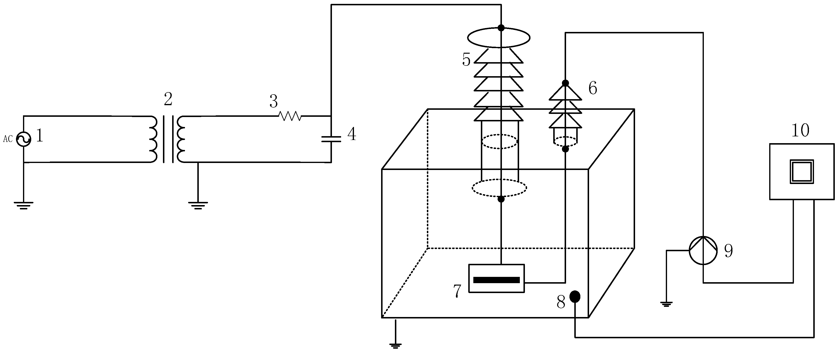
PD signals are extracted under different voltage conditions. The pulse current is collected by the current sensor with bandwidth 500 kHz–16 MHz. The Ultra High Frequency (UHF) signal is extracted by the UHF sensor with bandwidth 10 MHz–1000 MHz. The signal received is imported into the PD analyzer. The test condition is shown in

Table 1. Test condition of Partial Discharge models.

Partial Discharge (PD) Types	Initial Voltage/kV	Breakdown Voltage/kV	Testing Voltage/kV	Sample Number
Floating Discharge	2	7	3/4/5	20/20/20
Needle-Plate Discharge	8.8	12	9/10/11	20/20/20
Surface Discharge	3	10	5/6/7	20/20/20
Air-Gap Discharge	5	10	6/7/8	20/20/20

, with the experimental connection diagram shown in Figure 4.

The PD pulse is very weak, which can be easily disrupted by external interference. The laboratory environment is complicated, as it may be filled with electromagnetic interference caused by radio broadcasting and communication. Setting up voltage to 2 kV, one PD signal extracted in the laboratory as shown in Figure 5. Here, it is shown that the PD signal is obviously interfered by the noise in the laboratory, which makes it difficult to analyze directly.

3.2. Signal Processing

Figure 5 shows the original PD signal, which suffers from large background interference. To extract a valid PD signal, some necessary de-noising steps are needed. Since Wavelet Transform (WT) is suitable for processing a non-stationary signal with better time-frequency resolution performance [30]. Therefore, WT is employed for PD de-noising in this paper.

Two evaluation indexes are used for quantitative analysis of the de-noising quality, which are Noise Rejection Ratio (NRR) and Mean Square Error (MSE). NRR and MSE are defined according to Reference [31]:

$$NRR=10(\lg {\sigma }_1^2-\lg {\sigma }_2^2)$$

(22)

where ${\sigma }_1$ and ${\sigma }_2$ represent the noise deviation of the pre-treatment and post-treatment respectively. The deviation can be defined as:

$$\sigma =\sqrt{\frac{1}{Q}{\displaystyle \sum _{d=1}^Q{(S_d-\mu )}^2}}$$

(23)

where Q is the number of samples, S_d represents the d-th sampling signal, and $\mu$ is the mean of the signal.

$$MSE=\frac{1}{n}{\displaystyle \sum _{i=1}^n({\left|s_r(i)-{\widehat{s}}_r(i)\right|}^2)}$$

(24)

where $s_r(i)$ is the original PD reference signal, represented by the mean value of de-noised signals with Daubechies (db) 1–15 and 5-level decomposition. And ${\widehat{s}}_r$ is the signal after being de-noised by WT.

The higher the NRR, the more effective the de-noising result. The smaller the MSE, the more similarity between the original and the de-noised signal.

The wavelet threshold selection is of great importance to the de-noising effects. In this paper, the “hard” threshold function is adopted, as it gave better results when compared with the “soft” threshold [32]. Heursure is chosen as the wavelet threshold due to its good performance in signal de-noising.

Daubechies (db) is an orthogonal wavelet basis with compact support, which has a high similarity with PD signals. Therefore, db function is employed as wavelet basis for PD signal processing.

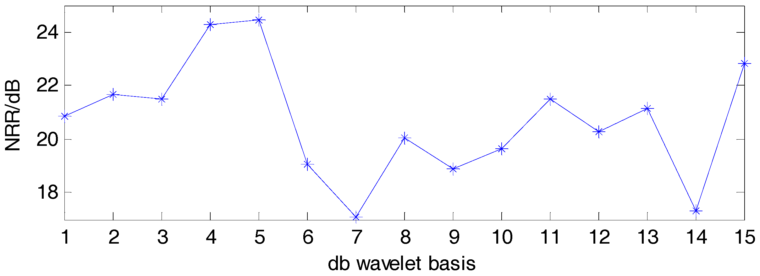
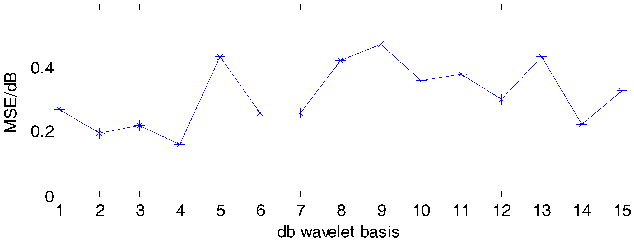
As shown in Figure 6 and Figure 7, with the 5-level decomposition, NRR and MSE variations with different db wavelet basis are obtained after 20 iterative calculations.

Figure 6 and Figure 7 show that the maximum of NRR is obtained with db5. Meanwhile, the minimum of MSE is obtained with db4. Considering that the value of MSE is larger with db5, db4 is selected as the wavelet basis.

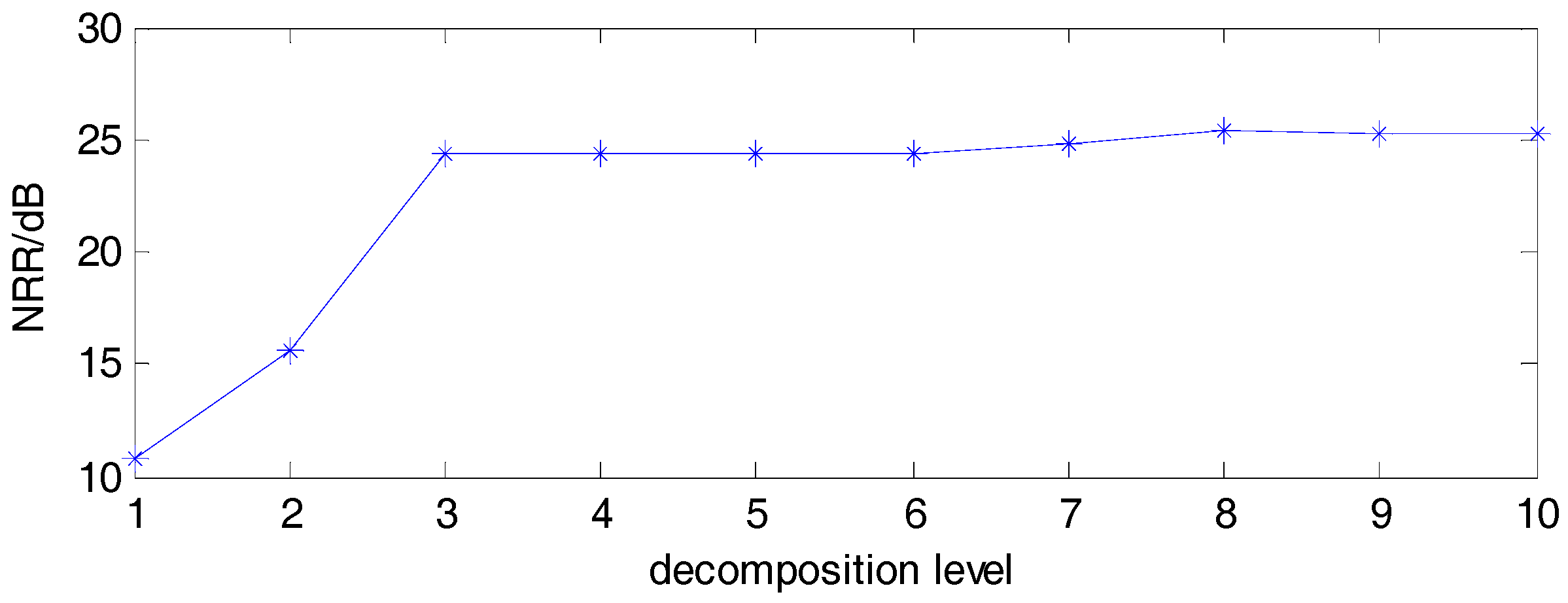
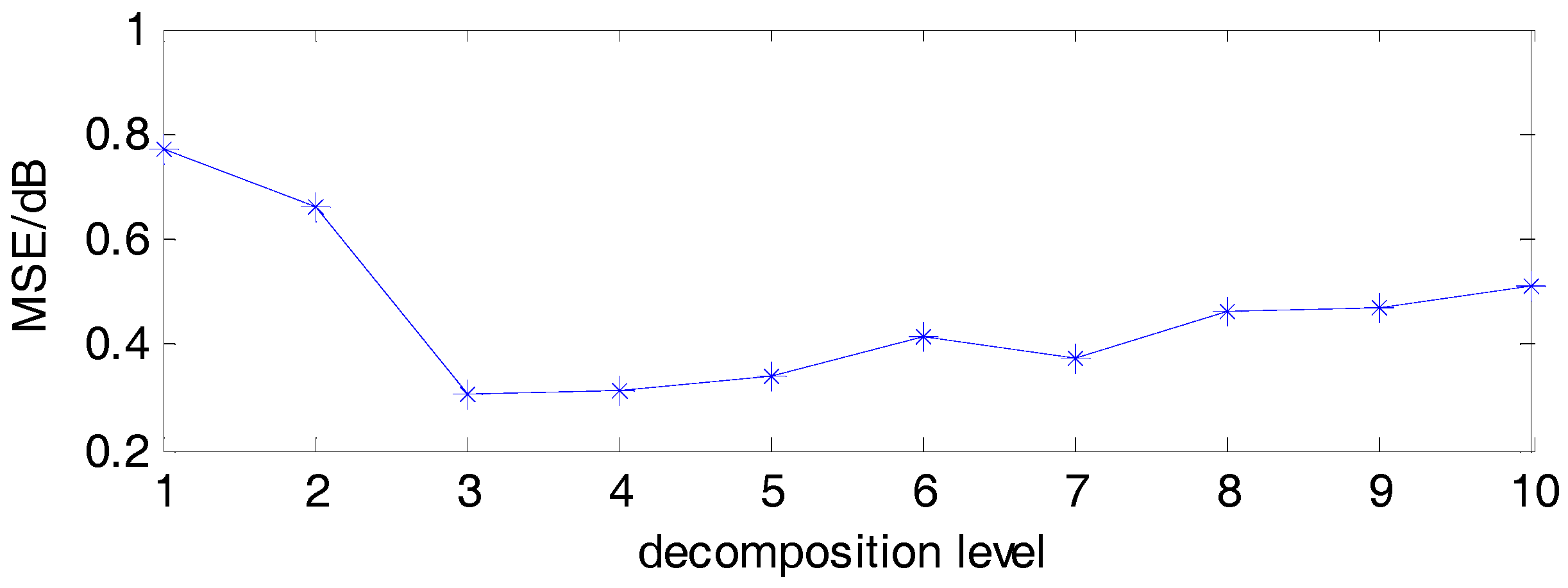
As shown in Figure 8 and Figure 9, using db4 wavelet, NRR and MSE variations with decomposition levels are obtained after 20 iterative calculations.

From the results shown in Figure 8 and Figure 9, the maximum of NRR is obtained at Level 8, while the minimum of MSE is obtained at Level 3. Considering that the computation complexity will increase with increasing level of decomposition, Level 3 is selected as the wavelet decomposition level.

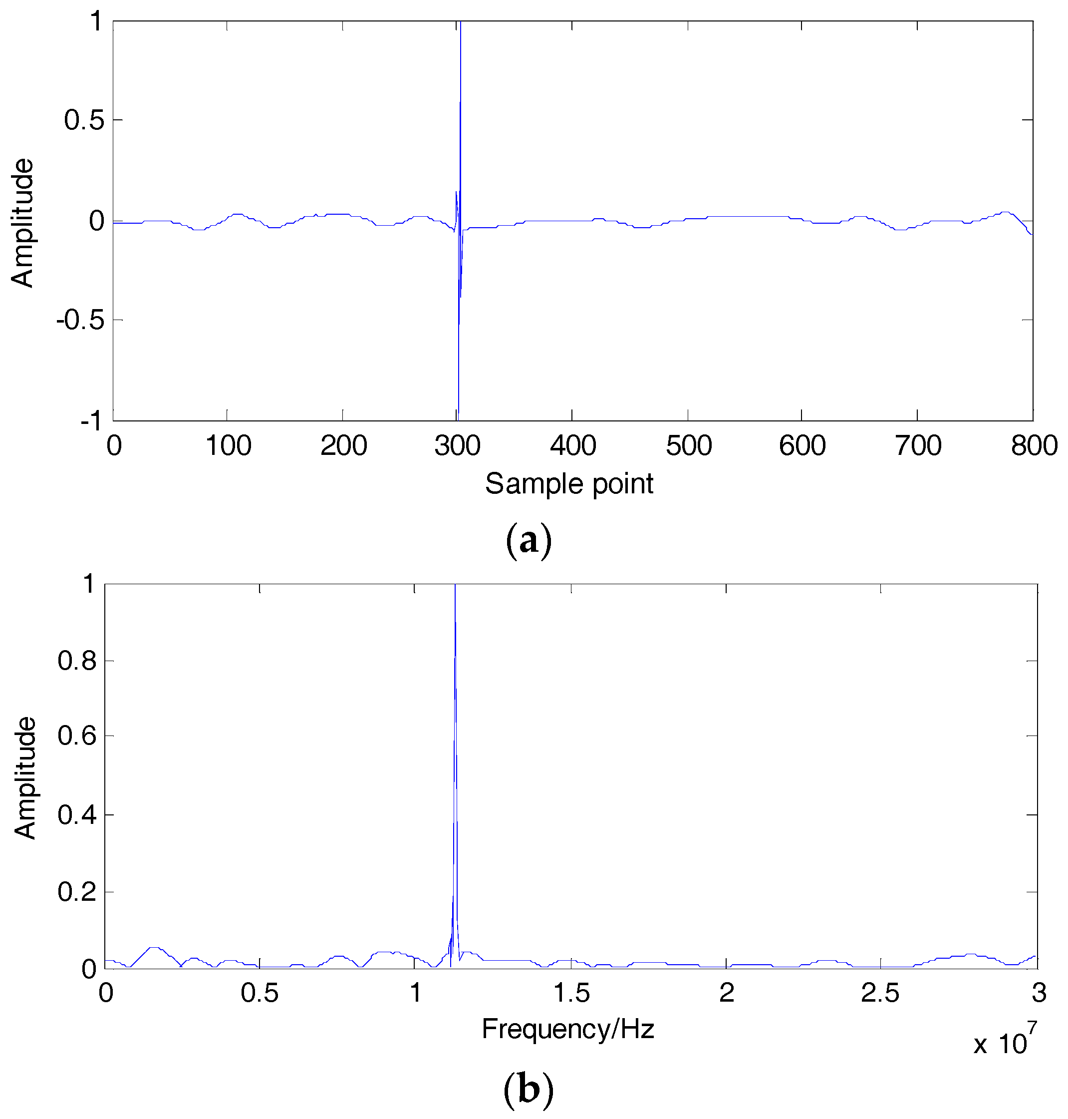
Through a series of experimental trials, the Daubechies mother wavelet “db4” with 3-level decomposition and a hard threshold are adopted in this study. The de-noised PD signal is shown in Figure 10. It is clear from these results that the background interference is effectively reduced.

After de-noising, different types of PD signals are presented in Figure 11.

3.3. Enseble Empirical Mode Decomposition Decomposition

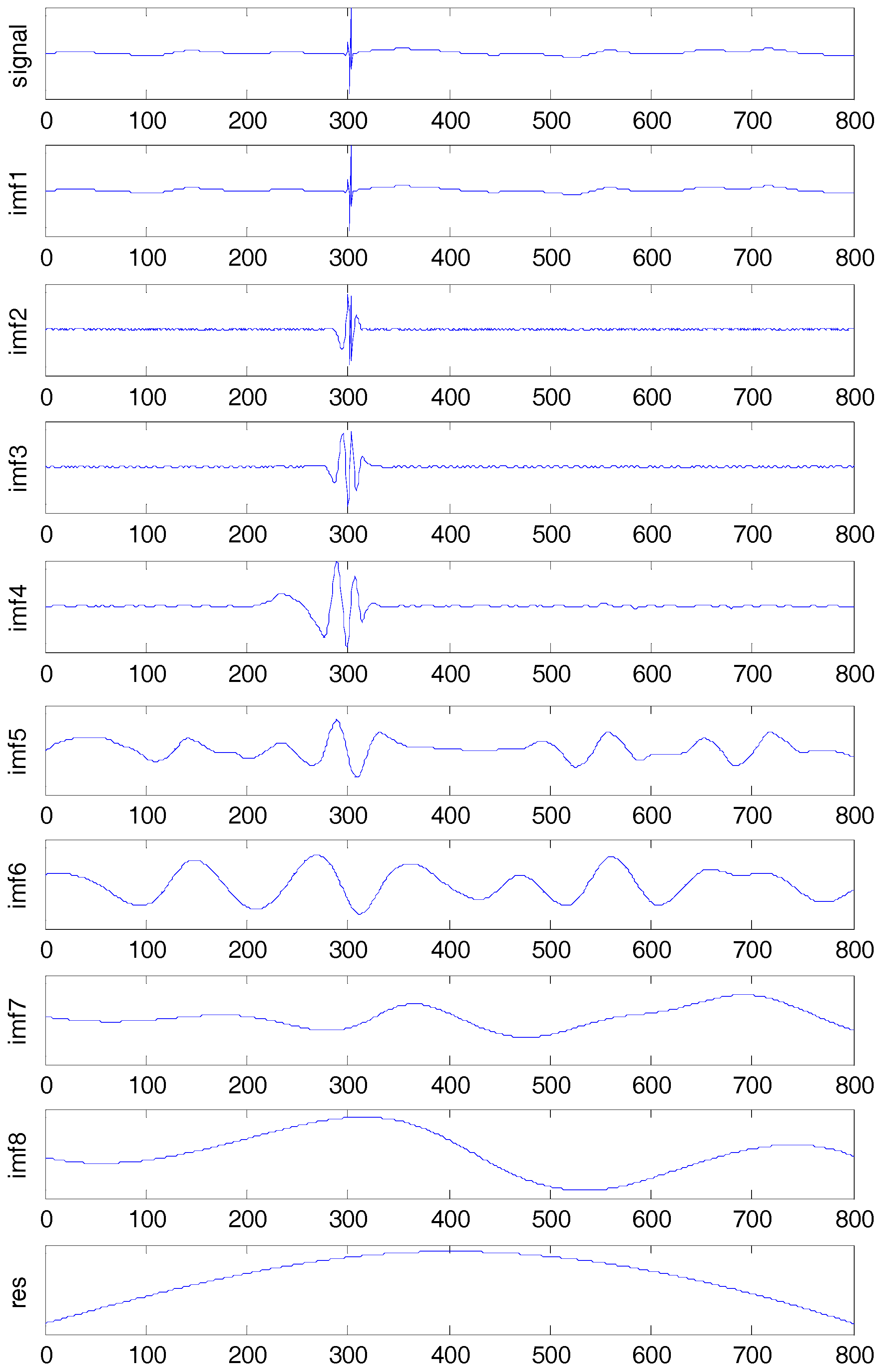
After de-noising, the PD signal decomposition result based on EEMD is presented in Figure 12. The standard deviation of white Gaussian noise is 0.1 and the repetitive number is 100. Figure 12 shows the IMF components in EEMD. The white noise makes each IMF maintain continuity in the time domain. EEMD decomposition method could clearly evaluate each component of the original PD signal.

3.4. IMF Selection

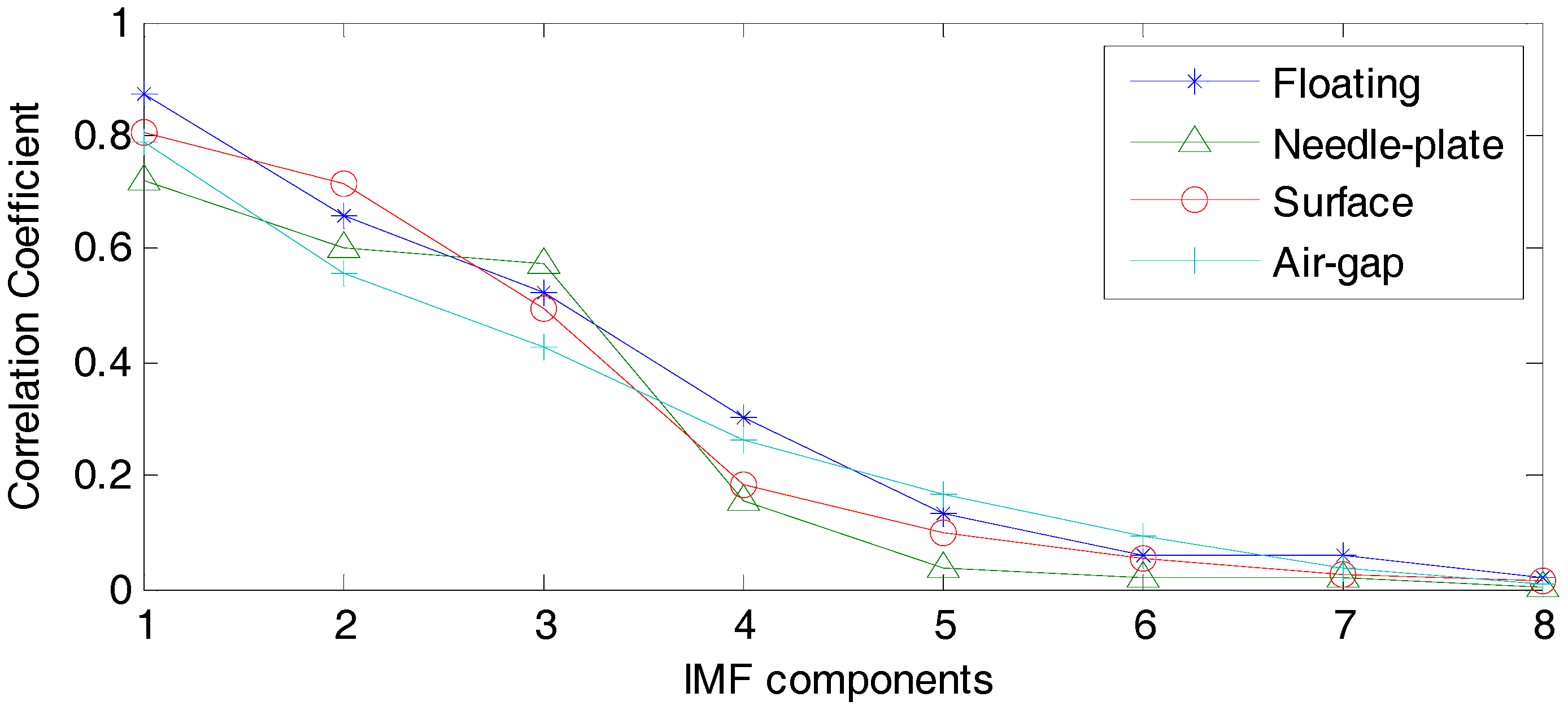
The real IMF components have good correlation with the original signal. On the other hand, the pseudo-components will only have poor correlation with the signal. Thus, the correlation coefficients between IMFs and the signal are used as a criterion to decide which IMFs should be retained and which IMFs should be rejected. To avoid rejecting some real IMFs with low amplitude, all IMFs as well as the signal will be normalized. The maximum of correlation coefficient is not more than 1. The calculated result of all the correlation coefficients and their relationship with IMF components are shown in Figure 13, as well as a solution for the IMF selection problem.

In Figure 13 it can be seen that the value of the correlation coefficient is decreasing with the increase of IMF components. The first three IMFs have good correlation with the original signal and have large correlation coefficients. From the fourth IMF to the eighth IMF component, the correlation coefficients are very small—less than 0.4. With IMF selection criterion, only the first three IMFs are retained and the others are rejected.

3.5. Sample Entropy Calculation

The value of Sample Entropy (SamEn) is related to the dimension, m, and the threshold, r. According to the study discussed in [33], the SamEn values are calculated with widely established values of m = 1 or m = 2, and with r a fixed value between 0.1 and 0.25 of the standard deviation of the individual subject time series. In this paper, SamEn is calculated with m = 1 and r = 0.2. The above procedure is used to calculate the characteristics of 240 PD signals obtained through laboratory experiments.

3.6. Partial Discharge Pattern Recognition Based on Relevance Vector Machine

In this study, Relevance Vector Machine (RVM) is applied to PD pattern recognition. The procedure is shown as follows.

(1)

PD characteristics are obtained in Section 3.5.

(2)

PD characteristics are sent to RVM as input vectors which are divided into two parts: training samples and testing samples.

(3)

As the One Against One (OAO) classifier is simple and has strong robustness [34], the PD classification model is set as an OAO model. Six classifiers are constructed shown in

Table 2. Partial Discharge classification model based on RVM.

PD Types	RVM1	RVM2	RVM3	RVM4	RVM5	RVM6
Floating Discharge	≥0.5	≥0.5	≥0.5	-	-	-
Surface Discharge	<0.5	-	-		≥0.5	≥0.5
Air-gap Discharge	-	<0.5	-	≥0.5	-	<0.5
Needle-plate Discharge	-	-	<0.5	<0.5	<0.5	-

. Each classifier is used to distinguish two different PD types. The judging index is set to 0.5. If the output is less than the judging index, then Type 1; otherwise Type 2.

(4)

Select proper kernel functions and kernel parameters.

(5)

The training samples are applied to train the RVM classification model.

(6)

Testing samples are sent to the trained RVM model for testing.

(7)

The test results show the final PD classification.

The recognition procedure can be seen in the flowchart in Figure 14.

4. Results and Analysis

4.1. Parameter Selection

During this experiment, four different types of PD signals were extracted in the laboratory. Sixty datasets of each type were used for analysis, of which 30 datasets were used for training and the rest were used for testing. To analyze the performance of different recognition methods, Back Propagation Neural Network (BPNN) [35], Probabilistic Neural Network (PNN) [36], Support Vector Machine (SVM) and Relevance Vector Machine (RVM) classifiers are employed. In the BPNN structure, the mapping of any continuous function could be achieved with one hidden layer. Therefore a one-hidden-layer structure is employed in this work. After iterative computation, the proper number of nodes in the hidden layer is set to four, and the optimal value of spread in PNN is set to 0.8. BPNN and PNN structure parameters are shown in

Table 3. Network Structure Parameters.

Classifiers	Input Layer Node Number	Hidden Layer Node Number	Output Layer Node Number
Back Propagation Neural Network (BPNN)	3	4	4
Neural Network (PNN)	3	*	4

* means there’s no hidden layer in PNN.

. The recognition accuracy with different kernel functions is shown in

Table 4. Recognition result with different kernel functions.

Kernel Functions	Recognition Accuracy (%)
	Support Vector Machine (SVM)	Relevance Vector Machine (RVM)
Linear	80.00	83.33
Polynomial	86.67	90.00
Radial Basis Function	96.67	93.33
Sigmoid	93.33	100.00

.

It can be concluded from Table 4 that different kernel functions of classifiers have diverse performance. For SVM, the optimal kernel function is Radial Basis Function (RBF). For RVM, the optimal kernel function is Sigmoid. The diverse performance is due to the different spatial feature between SVM and RVM. The feature space dimension for RBF is infinite, which is suitable for linear separation. Additionally, RBF meets Mercer conditions. Therefore, RBF is selected as the kernel function for SVM. Meanwhile Sigmoid is the kernel function with global features which is not restricted by Mercer conditions. As such, Sigmoid is selected as the kernel function for RVM.

Using two-fold cross validation, the optimal regularization coefficient of SVM is set to 0.3, and the kernel parameter is set to be 0.5. For RVM, the kernel parameter is set to be 0.2.

4.2. Performance Analysis

For both RVM and SVM, One Against One multi-class model is applied. The performance of different classifiers of SVM and RVM is given in

Table 5. Support Vector Machine (SVM) and Relevance Vector Machine (RVM) classification comparison.

Classifiers	Training Time/Second	Testing Time/Second	Vector Numbers	Recognition Accuracy (%)
SVM1	0.0632	0.002	11	86.67
RVM1	0.0405	9.02 × 10−4	9	86.67
SVM2	0.0528	0.0018	13	93.33
RVM2	0.0261	6.68 × 10−4	7	96.67
SVM3	0.0578	0.0015	11	96.67
RVM3	0.0355	8.92 × 10−4	6	96.67
SVM4	0.0738	0.0061	14	90.00
RVM4	0.0112	7.14 × 10−4	8	90.00
SVM5	0.0343	0.0016	13	93.33
RVM5	0.0205	6.90 × 10−4	7	93.33
SVM6	0.0669	0.0086	15	96.67
RVM6	0.0272	8.81 × 10−4	8	100.00

.

Table 5 shows that the training and testing time of RVM is faster when compared to SVM. The reason is that RVM model learning is based on Sparse Bayesian algorithm and the regularization coefficient is not necessarily validated. Therefore, the computation of parameter selection is less lengthy. Moreover, the vector number needed in RVM is smaller than that in SVM, resulting in a shorter testing time.

To compare the performance of different feature extraction methods, Statistics Parameters [5], Waveform Features [8], wavelet sample entropy (W-SamEn) [37], and EMD sample entropy (EMD-SamEn) are applied to PD analysis. In the EMD-SamEn method, the SamEn values are calculated with the first three IMFs. In W-SamEn method, after repeated tests, db4 is chosen as the wavelet basis and the decomposition level is set to 3.

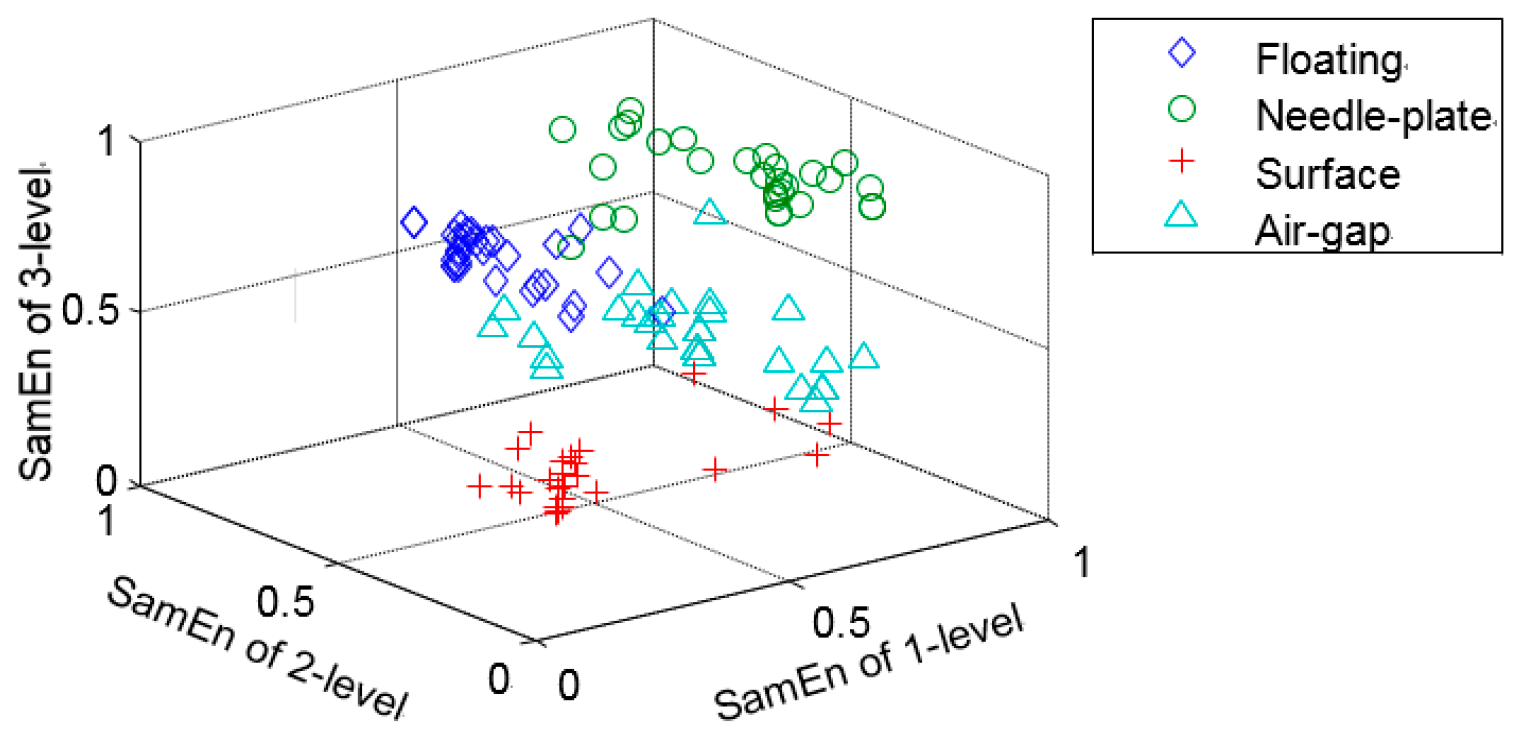
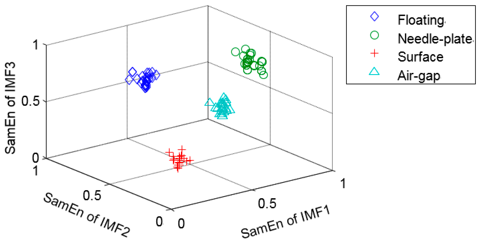
Based on the RVM classifier, the feature extraction effects of W-SamEn, EMD-SamEn and EEMD-SamEn are shown in Figure 15, Figure 16 and Figure 17.

Three axes in Figure 15 represent the extracted SamEn values from first three wavelet levels. Three axes in Figure 16 and Figure 17 represent the extracted SamEn values of the first three IMFs from EMD and EEMD, respectively. Figure 15 shows that, with W-SamEn method, PD types cannot be identified accurately and the classification boundaries are ambiguous. Wavelet basis function and decomposition level need to be determined manually, therefore the adaptability to signals is very poor, which causes poor performance. It can be seen in Figure 16 that EMD-SamEn method could get better recognition effect than W-SamEn. However, there is still no clear boundary between different PD types, as there is obvious mode mixing phenomenon during EMD decomposition of PD signals. Figure 17 shows that four different types of PD signals are classified effectively and there are clear boundaries between different PD types.

The performance of different feature extraction methods is shown in

Table 6. Recognition Performance.

Feature Types	Training Samples	Testing Samples	Recognition Accuracy (%)	Running Time/Second
Waveform Features	120	120	86.67	6.85 × 10−4
Statistics Parameters	120	120	96.67	3.51 × 10−3
W-SamEn	120	120	90.83	1.68 × 10−3
EMD-SamEn	120	120	96.67	7.28 × 10−4
EEMD-SamEn	120	120	100.00	7.32 × 10−4

.

Table 6 shows that different PD feature extraction methods have diverse recognition results and running times. Compared with other methods, the EEMD-SamEn method has the best recognition effect, with accuracy of 100.00%. Comparatively, the Waveform Feature has the worst recognition performance. It can be concluded from the Table 6 that, due to the attenuation and the interference in PD signal extraction, Waveform Feature has the worst recognition performance. Although the Statistics Parameters method has a better result, the running time is much longer because of the large number of parameters. In addition, the performance of W-SamEn method is not as good, since feature extraction errors exist during the selection of the wavelet basis and decomposition levels. PD feature extraction based on EMD-SamEn has better recognition accuracy with an average recognition accuracy of 96.67%. However, due to mode-mixing in the process of EMD, the classification accuracy is not satisfactory. The EEMD-SamEn method effectively avoids the selection of wavelet basis and decomposition levels, in addition to solving the problem of mode-mixing and virtual components. In conclusion, the proposed PD feature extraction method has the best recognition performance with an acceptable running time.

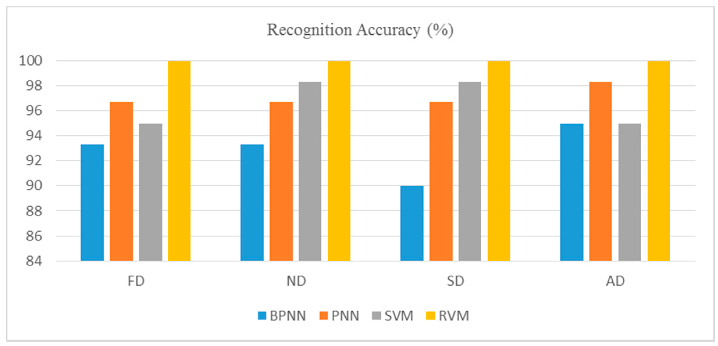
To verify the effectiveness of the proposed feature extraction approach, different classifiers are employed for PD type recognition. Sixty samples in each PD type are divided into two parts for training and testing, respectively. All samples of each PD type are labeled from No. 1–60. First, samples labeled No. 1–10 are used for testing, while others are used for training. Second, the training and testing samples are changed, with samples labeled No. 11–20 used for testing, while others are used for training. Finally, samples labeled No. 51–60 are used for testing, while others are used for training. Finally, all samples are used for both training and testing. With parameters extracted using the EEMD-SamEn method, the averaged recognition results based on different classifiers are shown in Figure 18.

It can be seen from Figure 18 that different PD types, including floating discharge (FD), needle-plate discharge (ND), surface discharge (SD), and air-gap discharge (AD), have diverse recognition performance using different classifiers. Due to the inherent problems of slow convergence rate and the tendency to be entrapped in a local minimum, BPNN has the worst recognition accuracy in SD. Comparing BPNN, PNN, and SVM, RVM has the best recognition effect with no mistaken sample in each PD type. Therefore, RVM has obvious advantages over other classifiers.

5. Conclusions

Partial Discharge fault recognition plays an important part in the insulation diagnosis of electrical equipment. In this study, Ensemble Empirical Mode Decomposition (EEMD) and Sample Entropy (SamEn) are combined for PD feature extraction. EEMD is employed for PD signal decomposition without mode-mixing or virtual components. Based on the IMFs of EEMD, Sample Entropy is calculated, which is sensitive to the properties of PD signals. The combination of EEMD and SamEn demonstrates that the proposed feature extraction method, combining the superiorities of both EEMD and Sample Entropy, is able to recognize the different PD types effectively. According to the results, the EEMD-SamEn method has obvious advantage over Waveform Features, Statistics Parameters, the W-SamEn and EMD-SamEn methods, as it solves the problems of high-dimension calculation and signal attenuation in traditional feature extraction methods. Thus, EEMD-SamEn is a practical tool for PD pattern recognition.

In this paper, different classifiers are employed for PD type recognition which include BPNN, PNN, SVM and RVM. Due to the particular model’s structure, RVM could avoid the choice of a regularization coefficient and restriction of Mercer conditions. Comparatively, RVM demonstrated the best performance with the average accuracy of RVM reaching an encouraging level.

It is worth noting that the PD experiment in this paper is aimed at a single PD defect. However, it is common that multiple defects appear at the same time in PD detection. Therefore, future study will focus on the multiple defects of PD signals. Considering that different measurement circuits and sensors may cause diverse PD features, signals from different measurement conditions should be extracted to verify the effectiveness of the proposed method in the future. Moreover, the work in this paper is accomplished in a laboratory environment, and it should be noted that there is a big difference between a laboratory environment and a field environment. The feature of on-site PD signals could be different from that of experimental signals. Additionally, in the real-world environment of PD condition maintenance, there is always insufficient time and a lack of experts to deal with the PD data, which are some important limitations of this research. For further consideration, large amounts of field-based PD data could be collected and analyzed.

References

- Kunicki, M.; Cichoń, A.; Borucki, S. Study on Descriptors of Acoustic Emission Signals Generated by Partial Discharges under Laboratory Conditions and in On-Site Electrical Power Transformer. Arch. Acoust. 2016, 41, 265–276. [Google Scholar] [CrossRef]
- Wang, M.H. Partial discharge pattern recognition of current transformers using an ENN. IEEE Trans. Power Deliv. 2017, 11, 1–17. [Google Scholar] [CrossRef]
- Gao, W.; Ding, D.; Liu, W.; Huang, X. Investigation of the Evaluation of the PD Severity and Verification of the Sensitivity of Partial Discharge Detection Using the UHF Method in GIS. IEEE Trans. Power Deliv. 2014, 29, 38–47. [Google Scholar]
- Wang, P.; Montanari, G.; Cavallini, A. Partial Discharge Phenomenology and Induced Aging Behavior in Rotating Machines Controlled by Power Electronics. IEEE Trans. Ind. Electron. 2014, 61, 7105–7112. [Google Scholar] [CrossRef]
- Chu, X.; Zhang, J.W.; Han, G. Partial discharge pattern recognition based on statistical parameters and multi-classifications SVM. Electr. Meas. Instrum. 2015, 52, 35–39. [Google Scholar]
- Ma, Z.; Zhou, C.; Hepburn, D.M.; Cowan, K. Fractal theory based pattern recognition of motor partial discharge. In Proceedings of the International Conference on Condition Monitoring and Diagnosis, Xi’an, China, 25–28 September 2016; pp. 881–884. [Google Scholar]
- Cui, L.; Chen, W.; Xie, B.; Du, J.; Long, Z.; Li, Y. Characteristic information extraction and developing process recognizing method of surface discharge in oil immersed paper insulation. In Proceedings of the IEEE International Conference on High Voltage Engineering and Application, Chengdu, China, 19–22 September 2015; pp. 1–4. [Google Scholar]
- Alvarez, F.; Ortego, J.; Garnacho, F.; Sanchez-Uran, M.A. A clustering technique for partial discharge and noise sources identification in power cables by means of waveform parameters. IEEE Trans. Dielectr. Electr. Insul. 2016, 23, 469–481. [Google Scholar] [CrossRef] [Green Version]
- Tang, J.; Liu, F.; Meng, Q.; Zhang, X.; Tao, J. Partial Discharge Recognition through an Analysis of SF 6 Decomposition Products Part 2: Feature Extraction and Decision Tree-based Pattern Recognition. IEEE Trans. Dielectr. Electr. Insul. 2012, 19, 37–44. [Google Scholar] [CrossRef]
- Huang, N.E.; Shen, Z.; Long, S.R.; Wu, M.C.; Shin, H.H.; Zheng, Q.; Yen, N.-C.; Tung, C.; Liu, H.H. The empirical mode decomposition and the Hilbert spectrum for nonlinear and non-stationary time series analysis. Proc. R. Soc. Lond. A Math. Phys. Sci. 1998, 454, 903–995. [Google Scholar] [CrossRef]
- Boudraa, A.O.; Cexus, J.C. EMD-based Signal Filtering. IEEE Trans. Instrum. Meas. 2007, 56, 2196–2202. [Google Scholar] [CrossRef]
- Wu, Z.; Huang, N.E. Ensemble empirical mode decomposition: A noise-assisted data analysis method. Adv. Adapt. Data Anal. 2009, 1, 1–41. [Google Scholar] [CrossRef]
- Fu, Y.; Jia, L.; Qin, Y.; Yang, J.; Ding, F. Fast EEMD Based AM-Correntropy Matrix and Its Application on Roller Bearing Fault Diagnosis. Entropy 2016, 18, 242. [Google Scholar] [CrossRef]
- Papadaniil, C.D.; Hadjileontiadis, L.J. Efficient Heart Sound Segmentation and Extraction Using Ensemble Empirical Mode Decomposition and Kurtosis Features. IEEE J. Biomed. Health Inform. 2014, 18, 1138–1152. [Google Scholar] [CrossRef] [PubMed]
- Kong, Y.B.; Guo, Y.; Wu, X. Double-impulse feature extraction of faulty hybrid ceramic ball bearings based on EEMD. J. Vib. Shock 2016, 35, 17–22. [Google Scholar]
- Patel, R.; Janawadkar, M.P.; Sengottuvel, S.; Gireesan, K.; Radhakrishnan, T.S. Effective Extraction of Visual Event-Related Pattern by Combining Template Matching With Ensemble Empirical Mode Decomposition. IEEE Sens. J. 2017, 17, 2146–2153. [Google Scholar] [CrossRef]
- Richman, J.S.; Lake, D.E.; Moorman, J.R. Sample Entropy. Methods Enzymol. 2004, 384, 172–184. [Google Scholar] [PubMed]
- Widodo, A.; Shim, M.C.; Caesarendra, W.; Yang, B.-S. Intelligent prognostics for battery health monitoring based on sample entropy. Expert Syst. Appl. 2011, 38, 11763–11769. [Google Scholar] [CrossRef]
- Mei, Z.; Ivanov, K.; Zhao, G.; Li, H.; Wang, L. An explorative investigation of functional differences in plantar center of pressure of four foot types using sample entropy method. Med. Biol. Eng. Comput. 2017, 55, 1–12. [Google Scholar] [CrossRef] [PubMed]
- Majidi, M.; Fadali, M.S.; Etezadi-Amoli, M.; Oskuoee, M. Partial discharge pattern recognition via sparse representation and ANN. IEEE Trans. Dielectr. Electr. Insul. 2015, 22, 1061–1070. [Google Scholar] [CrossRef]
- Mota, H.D.O.; Vasconcelos, F.H.; Castro, C.L.D. A comparison of cycle spinning versus stationary wavelet transform for the extraction of features of partial discharge signals. IEEE Trans. Dielectr. Electr. Insul. 2016, 23, 1106–1118. [Google Scholar] [CrossRef]
- Glowacz, A. Recognition of acoustic signals of induction motor using FFT, SMOFS-10 and LSVM. Maint. Reliab. 2015, 17, 569–574. [Google Scholar] [CrossRef]
- Tipping, M.E. Sparse Bayesian learning and the relevance vector machine. J. Mach. Learn. Res. 2001, 1, 211–244. [Google Scholar]
- Nguyen, D.D.; Le, H.S. Kinect Gesture Recognition: SVM vs. RVM. In Proceedings of the Seventh IEEE International Conference on Knowledge and Systems Engineering, Hanoi, Vietnam, 6–8 October 2016; pp. 395–400. [Google Scholar]
- Liu, Z.; Guo, W.; Tang, Z.; Chen, Y. Multi-Sensor Data Fusion Using a Relevance Vector Machine Based on an Ant Colony for Gearbox Fault Detection. Sensors 2015, 15, 21857–21875. [Google Scholar] [CrossRef] [PubMed]
- Hwang, S.; Jeong, M.K. Robust relevance vector machine for classification with variational inference. Ann. Oper. Res. 2015, 1–23. [Google Scholar] [CrossRef]
- MacKay, D.J.C. Bayesian interpolation. Neural Comput. 1992, 4, 415–447. [Google Scholar] [CrossRef]
- Gutten, M.; Korenciak, D.; Kucera, M.; Sebok, M.; Opielak, M.; Zukowski, P.; Koltunowicz, T.N. Maintenance diagnostics of transformers considering the influence of short-circuit currents during operation. Maint. Reliab. 2017, 19, 459–466. [Google Scholar] [CrossRef]
- Yang, Q.; Su, P.; Chen, Y. Comparison of Impulse Wave and Sweep Frequency Response Analysis Methods for Diagnosis of Transformer Winding Faults. Energies 2017, 10, 431. [Google Scholar] [CrossRef]
- Glowacz, A. DC Motor Fault Analysis with the Use of Acoustic Signals, Coiflet Wavelet Transform, and K-Nearest Neighbor Classifier. Arch. Acoust. 2015, 40, 321–327. [Google Scholar] [CrossRef]
- Shang, H.K.; Yuan, J.S.; Wang, Y.; Jin, S. Application of Wavelet Footprints Based on Translation-Invariant in Partial Discharge Signal Detection. Trans. China Electrotech. Soc. 2013, 28, 33–40. [Google Scholar]
- Altay, Ö.; Kalenderli, Ö. Wavelet base selection for de-noising and extraction of partial discharge pulses in noisy environment. IET Sci. Meas. Technol. 2015, 9, 276–284. [Google Scholar] [CrossRef]
- Pincus, S.M. Assessing serial irregularity and its implications for health. Ann. N. Y. Acad. Sci. 2001, 954, 245–267. [Google Scholar] [CrossRef] [PubMed]
- Liu, C.Y. Research and Application on the Multi-classification of Relevance Vector Machine Algorithm. Ph.D. Thesis, Harbin Engineering University, Harbin, China, 2013. [Google Scholar]
- Glowacz, A.; Glowacz, Z. Diagnosis of the three-phase induction motor using thermal imaging. Infrared Phys. Technol. 2016, 81, 7–16. [Google Scholar] [CrossRef]
- Kusy, M.; Zajdel, R. Application of Reinforcement Learning Algorithms for the Adaptive Computation of the Smoothing Parameter for Probabilistic Neural Network. IEEE Trans. Neural Netw. Learn. Syst. 2015, 26, 2163–2175. [Google Scholar] [CrossRef] [PubMed]
- Alcaraz, R.; Vaya, C.; Cervigon, R.; Sanchez, C.; Rieta, J.J. Wavelet sample entropy: A new approach to predict termination of atrial fibrillation. In Proceedings of the 2006 Computers in Cardiology, Valencia, Spain, 17–20 September 2006; pp. 597–600. [Google Scholar]
Figure 1.
Flow diagram of feature extraction based on Ensemble Empirical Mode Decomposition (EEMD) and Sample Entropy (SamEn).
Figure 2.
Partial Discharge (PD) models. (a) Floating discharge (FD); (b) Needle-plate discharge (ND); (c) Surface discharge (SD); (d) Air-gap discharge (AD).
Figure 3.
Photograph of experimental setup.
Figure 4.
The connection diagram of the Partial Discharge experiment. (1) AC power source; (2) step up transformer; (3) resistance; (4) capacitor; (5) high voltage bushing; (6) small bushing; (7) PD model; (8) Ultra High Frequency (UHF) sensor; (9) current sensor; (10) console.
Figure 5.
Original Partial Discharge signal. (a) Time domain; (b) Frequency domain.
Figure 6.
Noise Rejection Ratio (NRR) with different db wavelet basis.
Figure 7.
Mean Square Error (MSE) variation with different db wavelet basis.
Figure 8.
Noise Rejection Ratio (NRR) variation with decomposition levels.
Figure 9.
Mean Square Error (MSE) variation with decomposition levels.
Figure 10.
De-noised Partial Discharge signal. (a) Time domain signal; (b) Frequency domain signal.
Figure 11.
Different types of Partial Discharge signals; (a) FD (b) ND; (c) SD (d) AD.
Figure 12.
EEMD decomposition.
Figure 13.
Intrinsic Mode Function (IMF) variation with correlation coefficient.
Figure 14.
Partial Discharge recognition procedure based on Relevance Vector Machine.
Figure 15.
Partial Discharge feature extraction effect based on wavelet sample entropy (W-SamEn).
Figure 16.
Partial Discharge feature extraction effect based on Empirical Mode Decomposition (EMD) sample entropy (EMD-SamEn).
Figure 17.
Partial Discharge feature extraction effect based on Ensemble Empirical Mode Decomposition sample entropy (EEMD-SamEn).
Figure 18.
Recognition Results of Different Classifiers.