The KCOD Model on (3,4,6,4) and (34,6) Archimedean Lattices

Dietrich Stauffer Computational Physics Lab, Departamento de Física Universidade Federal do Piauí, Teresina 64049-550, Brazil
Entropy 2017, 19(9), 459; https://doi.org/10.3390/e19090459
Submission received: 23 July 2017
/
Revised: 18 August 2017
/
Accepted: 30 August 2017
/
Published: 31 August 2017
(This article belongs to the Special Issue Statistical Mechanics of Complex and Disordered Systems)
Abstract
:Through Monte Carlo simulations, we studied the critical properties of kinetic models of continuous opinion dynamics on () and () Archimedean lattices. We obtain and the critical exponents’ ratio from extensive Monte Carlo studies and finite size scaling. The calculated values of the critical points and Binder cumulant are and ; and and for () and () lattices, respectively, while the exponent ratios , and are, respectively: , , and for (); and , , and for () lattices. Our new results agree with majority-vote model on previously studied regular lattices and disagree with the Ising model on square-lattice.
1. Introduction
The study of the behavior of individuals in a society by physicists is known as sociophysics, having as the main contributor in this new research area Serge Galam who introduced the use of local majority rules to study voting systems as bottom-up democratic voting in hierarchical structures [1,2,3,4]. Although sociophysics was rejected by some physicists in the eighties [5], it has today become an active field of research among physicists all over the world [3,6,7].
In this same context and based on the criterion of Grinstein et al. [8] (where a nonequilibrium model presenting up–down symmetry in two-state dynamic systems implies the same critical behavior (same universality class) as the equilibrium Ising model), Oliveira [9] proposed a nonequilibrium version of Ising model called majority vote model (MVM). On two-dimensional regular lattices, this presents a second-order phase transition with critical exponents , , , as for [10,11] the equilibrium Ising model [12,13].
Lima and Malarz [14] studied the MVM on () and () Archimedean lattices (ALs). On these lattices, they found a second-order phase transition with exponent ratios , , for () and , , for (), see Table 1.
A multiagent model for opinion formation in society by modifying kinetic exchange dynamics studied in the context of income, money, or wealth distributions in a society where a spontaneous symmetry-breaking transition to polarized opinion states starting from nonpolarized opinion states was proposed by M. Lallouache et al. [15].
A model of continuous opinion dynamics (KCOD) was proposed by Biswas et al. [16] in 2012. In the KCOD model, the mutual interactions can be both positive and negative and a single parameter p denoting the fraction of negative interactions was considered in order to characterize the different types of distributions for the mutual interactions. Numerical simulations of the continuous version of this model indicate the existence of a universal continuous phase transition at with exponents of mean field (, , and ) (see also [17]).
The KCOD model on square and cubic lattices (2D and 3D) was studied by Mukherjee and Chatterjee [19]. Their numerical results indicate that the critical behavior of the KCOD model is the same as that of the Ising model in the corresponding dimensions.
Recently, C. Anteneodo and N. Crokidakis [20] studied a model of like KCOD model in the presence of a social temperature. The critical behavior of this model showed three different kinds of collective states (symmetric, asymmetric, and neutral) and nonequilibrium transitions between them (see also [21,22]).
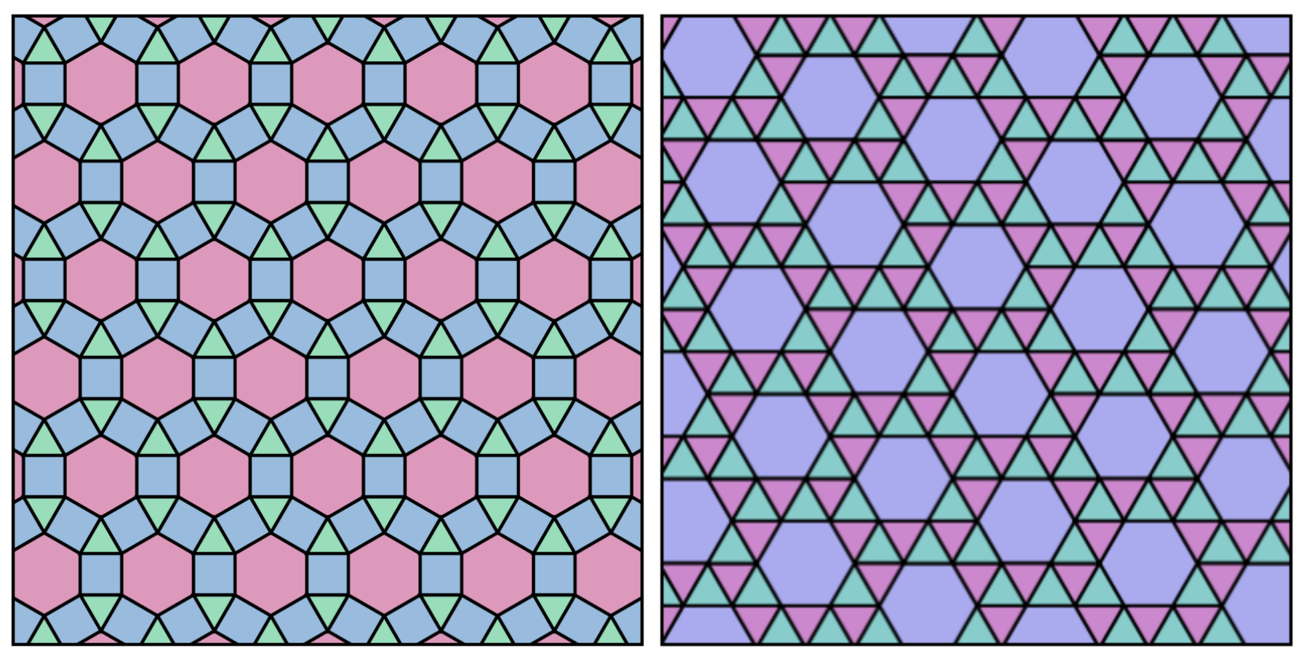
In this work, we studied the KCOD on two Archimedean lattices—namely, and —through extensive Monte Carlo simulations. The topologies of , and AL are presented in Figure 1. The AL are vertex transitive graphs that can be embedded in a plane such that every face is a regular polygon. Kepler showed that there are exactly eleven such graphs. The AL are labeled according to the sizes of faces incident to a given vertex. The face sizes are sorted, starting from the face for which the list is the smallest in lexicographical order. In this way, the square lattice gets the name (abbreviated to ), honeycomb is called , and Kagome is . Here, we also compared our results with those of the MVM made on and AL.
2. Model and Simulations
The KCOD [16] model is defined as follows: A set of agents (individuals) with continuous opinion variables is situated on every node of the () and () AL with sites. The opinion of an individual i at time t takes the values in the range , in a system of N agents. Here, the opinions change out of pair-wise interactions via mutual influences/couplings as:
where the interactions are pair-wise interactions between nearest neighbors, which implies no sum over the index j, and are real random variables. In the above dynamics (Equation (1)), an agent i updates his opinion by interacting with agent j and is influenced by the mutual influence term . Here, j is selected randomly from one of the nearest neighbors. Unlike other models (such as Ising model and MVM) that present up–down symmetry [23], in the KCOD model the opinions are bounded (i.e., ). If the opinion value of an agent becomes higher (lower) than +1 (−1), then it is made equal to +1 (−1) to preserve this bound. This bound, along with Equation (1), defines the dynamics of the model. Here, is a continuous random variable defined in the range [−1, +1]. The ordering in the system is measured by the quantity , the average opinion. Changing the fraction p of negative interactions, one can observe a symmetry breaking transition between an ordered and a disordered phase below a particular value of the parameter p, the system orders (giving a non-zero, finite value of the order parameter O (opinion), defined in the following), while a disordered phase exists above ().
To study the critical behavior of the model, we are interested in the average opinion O, order parameter fluctuations OF, and the reduced fourth-order cumulant of the O (herein named as O4), defined as
where stands for time averages, computed at the steady states. The results are averaged over the independent simulations.
The above-mentioned quantities are functions of the disorder parameter p, and obey the finite-size scaling relations
where , , and are the usual critical exponents, are the finite-size scaling functions with
being the scaling variable. Therefore, from the size dependence of O and OF, we obtained the exponent ratios (O) and (OF). The maximum value of susceptibility also scales as . Moreover, the value of for which OF has a maximum is expected to scale with the system size as
Therefore, the relations (3c) and (4) may be used to get the exponent . We also evaluate the effective dimensionality, , from the hyperscaling hypothesis
Monte Carlo simulations were performed on and () AL with various systems of size 384, 1536, 6144, 24, 576, and 98, 304 for and AL. It takes Monte Carlo steps (MCS) to let the system reach the steady state, and then the time averages are calculated over the next MCS. One MCS is accomplished after N attempts to update the opinions of agents i and j, considering the evolution Equations (1) and (2). The results are averaged over independent simulation runs for each lattice and for given set of parameters .
3. Results and Discussion
In all simulations described in the previous section, we used sequential Monte Carlo steps and considered continuous values within the interval [−1,+1]. Here, we only discuss the case when are annealed (i.e., they change with time).
Figure 2 displays the dependence of the opinion O, OF, and O4 on the disorder parameter p, obtained from simulations on and AL with L ranging from to . The shape of , , and curves for a given value of L indicate the occurrence of a second-order phase transition in the system. The phase transition occurs at the value of the critical disorder parameter . This critical disorder parameter is estimated as the point where the curves of the Binder cumulant for different system sizes N intercept each other [24]. The corresponding value of is represented by . Then, we obtained and ; and for , and AL, respectively.
To make the critical point on the x-axis more qualitatively visible than the traditional plot of (y-axis), Figure 3 displays the dependence of instead dependence of of the disorder parameter p, obtained from simulations on and AL.
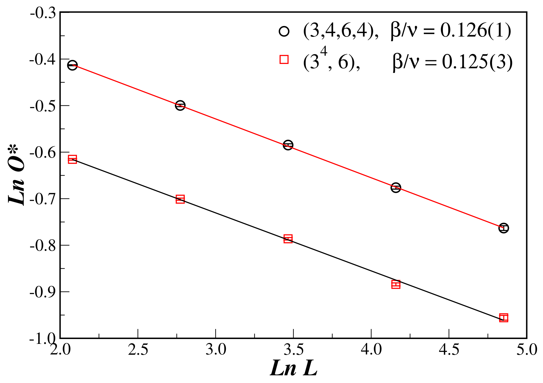
In Figure 4, we plot the opinion vs. L. The fits of the curves correspond to the exponent ratio according to relation Equation (3a); see Table 2.
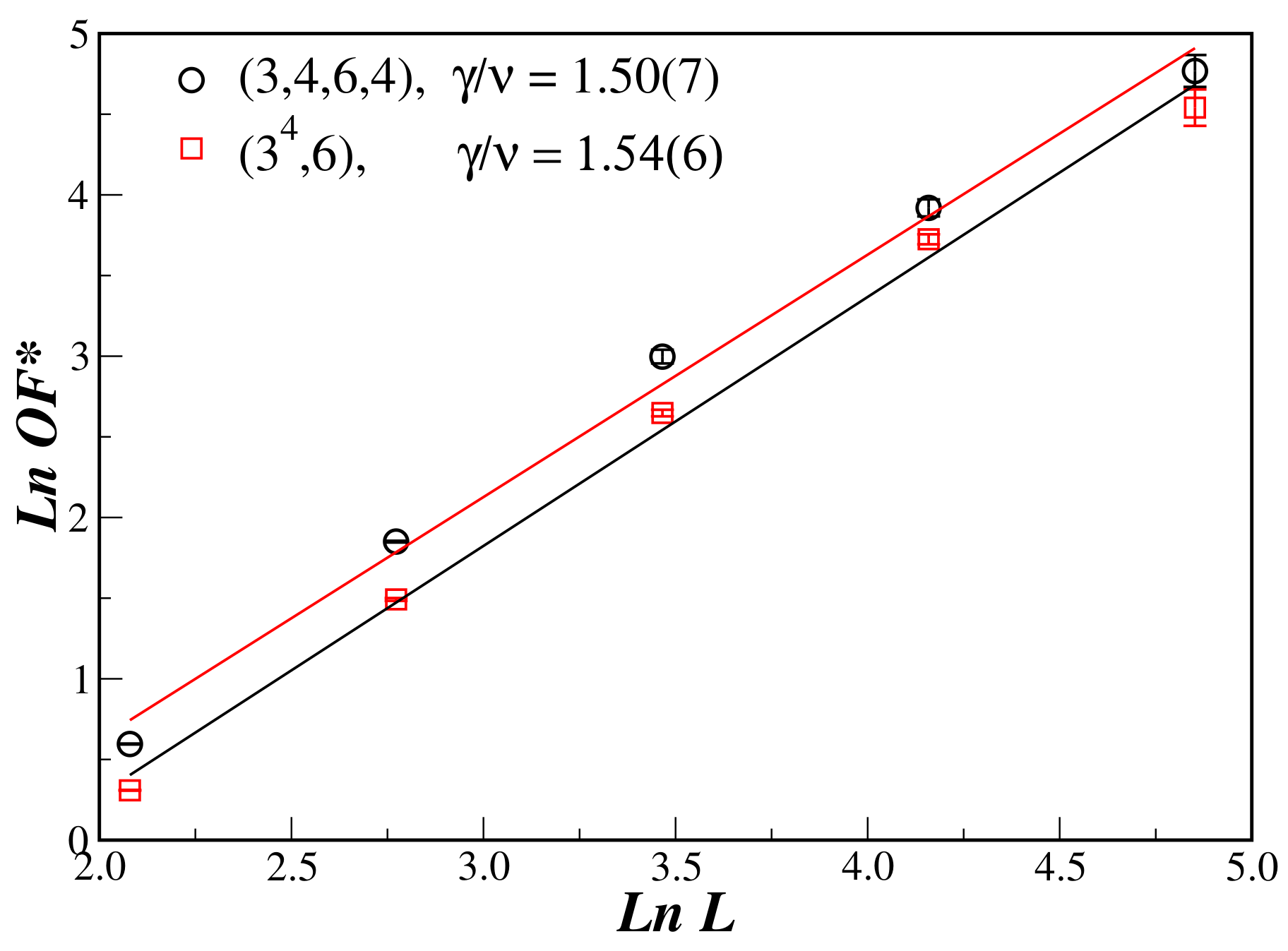
The Figure 5 displays the log-log plot of the at as a function of the lattice size L. The slopes of curves correspond to the exponent ratio according to Equation (3b). The numerical estimates are for and for AL.
In Figure 6 we present the exponent ratios at as for and for AL.
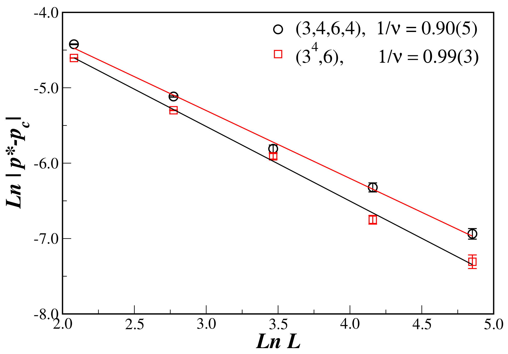
In Figure 7, we used the scaling relation Equation (4) and obtained the exponent ratio . The calculated values of the exponent are in Table 2.
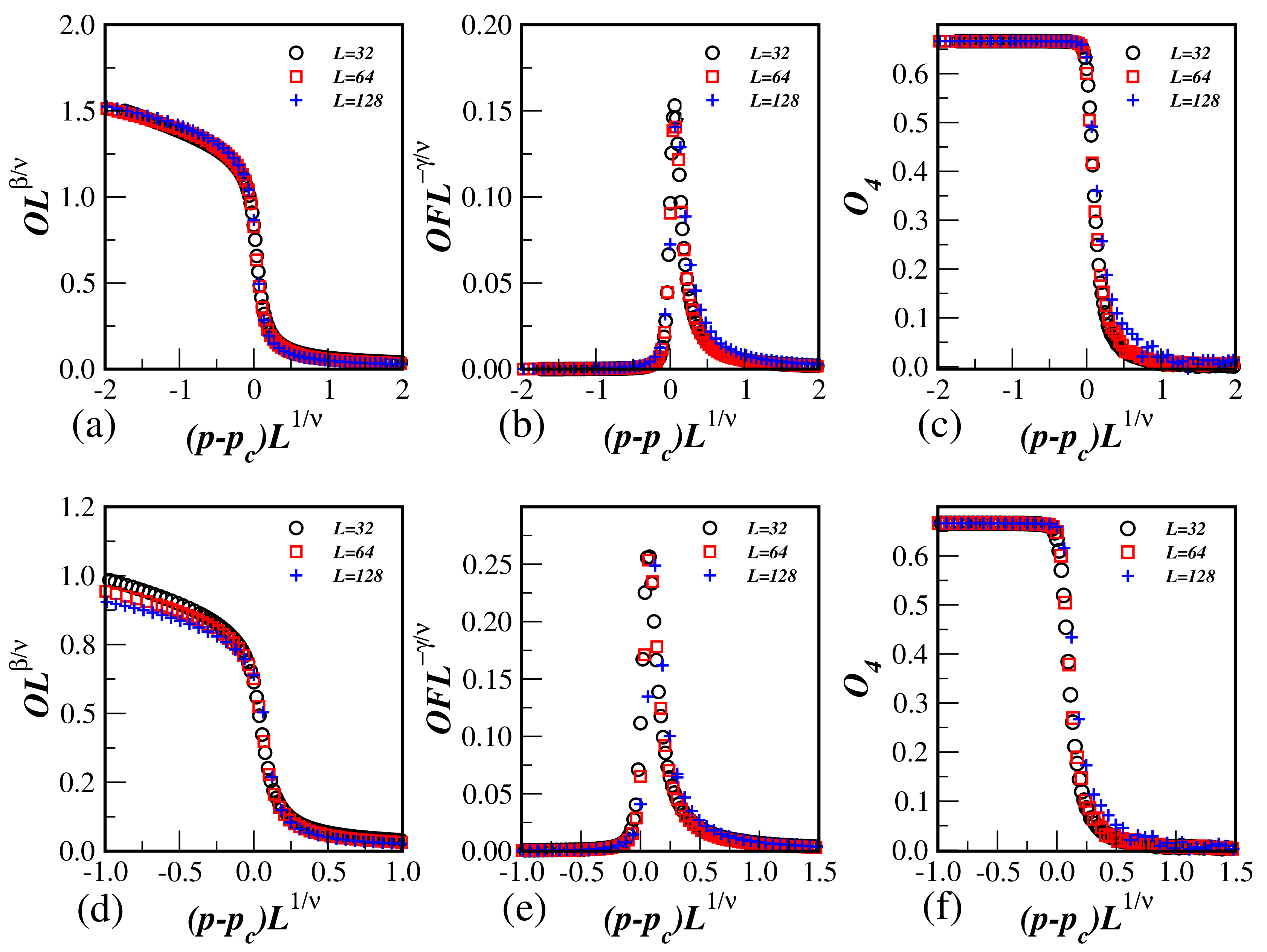
In Figure 8a,d we plot versus using the critical exponent ratios , , and and for and . In Figure 8b,e we plot versus using the critical exponent ratios and and and for and . In Figure 8c,f we plot versus using the critical exponent and for and . The excellent curve collapse for distinct system sizes corroborates our estimated values for and exponent ratios , , and .
The resulting critical exponents and disorder parameters are collected in Table 2. One can also see that the exponent ratios , , are very close to MVM (Table 1), as expected by Grinstein criterion for regular lattices [8]. They are different from obtained for a regular Ising model, but obey hyperscaling relation (within the error bars). Equation (5) yields effective dimensionality of systems for and for . The KCOD on those two AL has the effective dimensionality close to MVM for () and for () AL (see Table 1 and Table 2). The results of simulations are collected in Table 2.
4. Conclusions
We studied a nonequilibrium KCOD model through extensive Monte Carlo simulations on and AL. On these lattices, the KCOD shows a second-order phase transition. Our Monte Carlo simulations suggest that the effective dimensionality is close to two; i.e., that hyperscaling relation may be valid.
Finally, we remark that the critical exponents , , and for KCOD on and AL are very close to the MVM model on and AL [14] (see Table 1 and Table 2). Therefore, the exponent ratio and differs from 2D Ising model while and for MVM is a weak indication and for KCOD is a strong indication for Ising. Therefore, the KCOD model does not belong to the Ising universality class [12,18]. Thus, our results agree partially with Grinstein.
Acknowledgments
F.W.S. Lima thanks Dietrich Stauffer for many suggestions and fruitful discussions during the development of this work. We thank Brazilian agency (CNPq) for financial support. This work also was supported by system Silicon Graphics Internacional (SGI) Altix 1350 (CENAPAD.UNICAMP-USP, SP-BRAZIL).
Conflicts of Interest
The author declares no conflict of interest.
References
- Galam, S. Majority rule, hierarchical structures, and democratic totalitarianism: A statistical approach. J. Math. Psychol. 1986, 30, 426–434. [Google Scholar] [CrossRef]
- Galam, S. Social paradoxes of majority rule voting and renormalization group. J. Stat. Phys. 1990, 61, 943–951. [Google Scholar] [CrossRef]
- Fortunato, S.; Macy, M.; Redner, S. Editorial. J. Stat. Phys. 2013, 151, 1–8. [Google Scholar] [CrossRef]
- Galam, S. The drastic outcomes from voting alliances in three-party democratic voting (1990 → 2013). J. Stat. Phys. 2013, 151, 46–68. [Google Scholar]
- Galam, S. Sociophysics: A personal testimony. Physica A 2004, 336, 49–55. [Google Scholar] [CrossRef]
- Stauffer, D. A Biased Review of Sociophysics. J. Stat. Phys. 2013, 151, 9–20. [Google Scholar] [CrossRef]
- Galam, S. Sociophysics: A Physicist’s Modeling of Psycho-Political Phenomena; Springer: Berlin, Germany, 2012. [Google Scholar]
- Grinstein, G.; Jayaprakash, C.; He, Y. Statistical Mechanics of Probabilistic Cellular Automata. Phys. Rev. Lett. 1985, 55, 2527. [Google Scholar] [CrossRef] [PubMed]
- De Oliveira, M.J. Isotropic majority-vote model on a square lattice. J. Stat. Phys. 1992, 66, 273–281. [Google Scholar] [CrossRef]
- Santos, M.A.; Teixeira, S. Anisotropic voter model. J. Stat. Phys. 1995, 78, 963–970. [Google Scholar] [CrossRef]
- Crochik, L.; Tomé, T. Entropy production in the majority vote model. Phys. Rev. E 2005, 72, 057103. [Google Scholar] [CrossRef] [PubMed]
- Hasenbusch, M. Monte Carlo studies of the three-dimensional Ising model in equilibrium. Int. J. Mod. Phys. C 2001, 12, 911–1009. [Google Scholar] [CrossRef]
- Binney, J.J.; Dowrick, N.J.; Fisher, A.J.; Newman, M.E.J. A Theory of Critical Phenomena. An Introduction to the Renormalization Group; Clarendon Press: Oxford, UK, 1992. [Google Scholar]
- Lima, F.W.S.; Malarz, K. Majority-vote model on (3, 4, 6, 4) and (34, 6) Archimedean Lattices. Int. J. Mod. Phys. C 2006, 17, 1273–1283. [Google Scholar] [CrossRef]
- Lallouache, M.; Chakrabarti, A.S.; Chakraborti, A.; Chakrabarti, B.K. Opinion formation in kinetic exchange models: Spontaneous symmetry-breaking transition. Phys. Rev. E. 2010, 82, 056112. [Google Scholar] [CrossRef] [PubMed]
- Biswas, S.; Chatterjee, A.; Sen, P. Disorder induced phase transition in kinetic models of opinion dynamics. Physica A 2012, 391, 3257–3265. [Google Scholar] [CrossRef]
- Sen, P. Nonconservative kinetic exchange model of opinion dynamics with randomness and bounded confidence. Phys. Rev. E 2012, 86, 016115. [Google Scholar] [CrossRef] [PubMed]
- Temperley, H.N.V. Two-dimensional Ising models. In Phase Transitions and Critical Phenomena; Domb, C., Green, M.S., Eds.; Academic Press: London, UK, 1972; Volume 1. [Google Scholar]
- Mukherjee, S.; Chatterjee, A. Disorder induced phase transition in an opinion dynamics model: Results in 2 and 3 dimensions. Phys. Rev. E 2016, 94, 062317. [Google Scholar] [CrossRef] [PubMed]
- Anteneodo, C.; Crokidakis, N. Symmetry breaking by heating in a continuous opinion model. Phys. Rev. E 2017, 95, 042308. [Google Scholar] [CrossRef] [PubMed]
- Vieira, A.R.; Anteneodo, C.; Crokidakis, N. Consequences of nonconformist behaviors in a continuous opinion model. J. Stat. Mech. Theory Exp. 2016, 2016, 023204. [Google Scholar] [CrossRef]
- Yu, Y.; Xiao, G.; Li, G.; Tay, W.P.; Teoh, H.F. Opinion diversity and community formation in adaptive networks. arXiv, 2017; arXiv:1703.02223. [Google Scholar]
- Biswas, S.; Chandra, A.K.; Chatterjee, A.; Chakrabarti, B.K. Phase transitions and non-equilibrium relaxation in kinetic models of opinion formation. J. Phys. Conf. Ser. 2011, 297, 012004. [Google Scholar]
- Binder, K.; Heermann, D.W. Monte Carlo Simulation in Statistical Phyics; Springer: Berlin, Germany, 1988. [Google Scholar]
Figure 1.
Picture of the (left) and (right) AL.

Figure 2.
(Color online). The opinion O, , and , as a function of the parameter p, for lattice size , 16, 32, 64, and 128, and sites for (a–c) and Archimedean lattice (AL) (d–f).
Figure 2.
(Color online). The opinion O, , and , as a function of the parameter p, for lattice size , 16, 32, 64, and 128, and sites for (a–c) and Archimedean lattice (AL) (d–f).
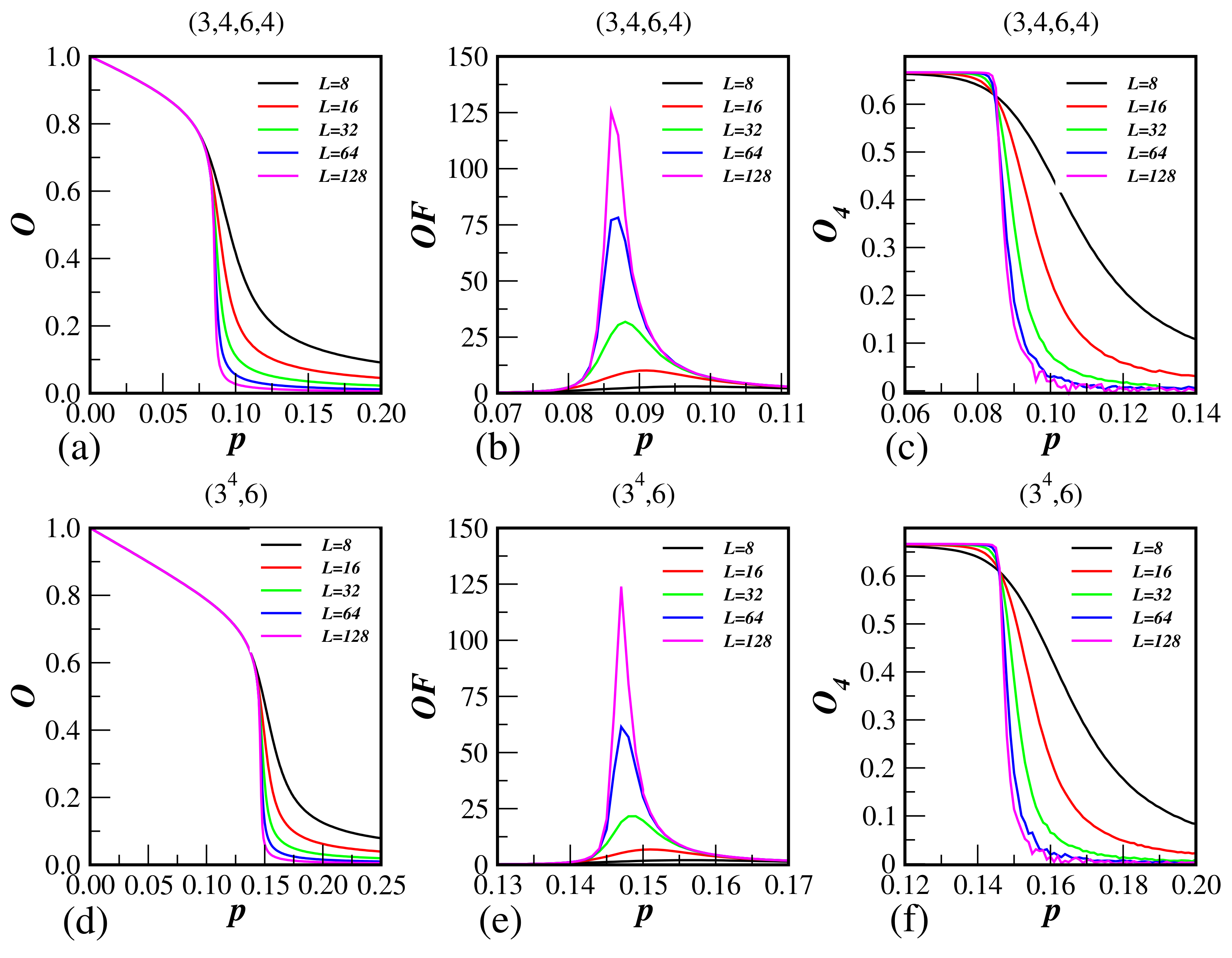
Figure 3.
(Color online). The as a function of the parameter p, for , 16, 32, 64, and 128 lattice sizes, and for and AL.
Figure 3.
(Color online). The as a function of the parameter p, for , 16, 32, 64, and 128 lattice sizes, and for and AL.
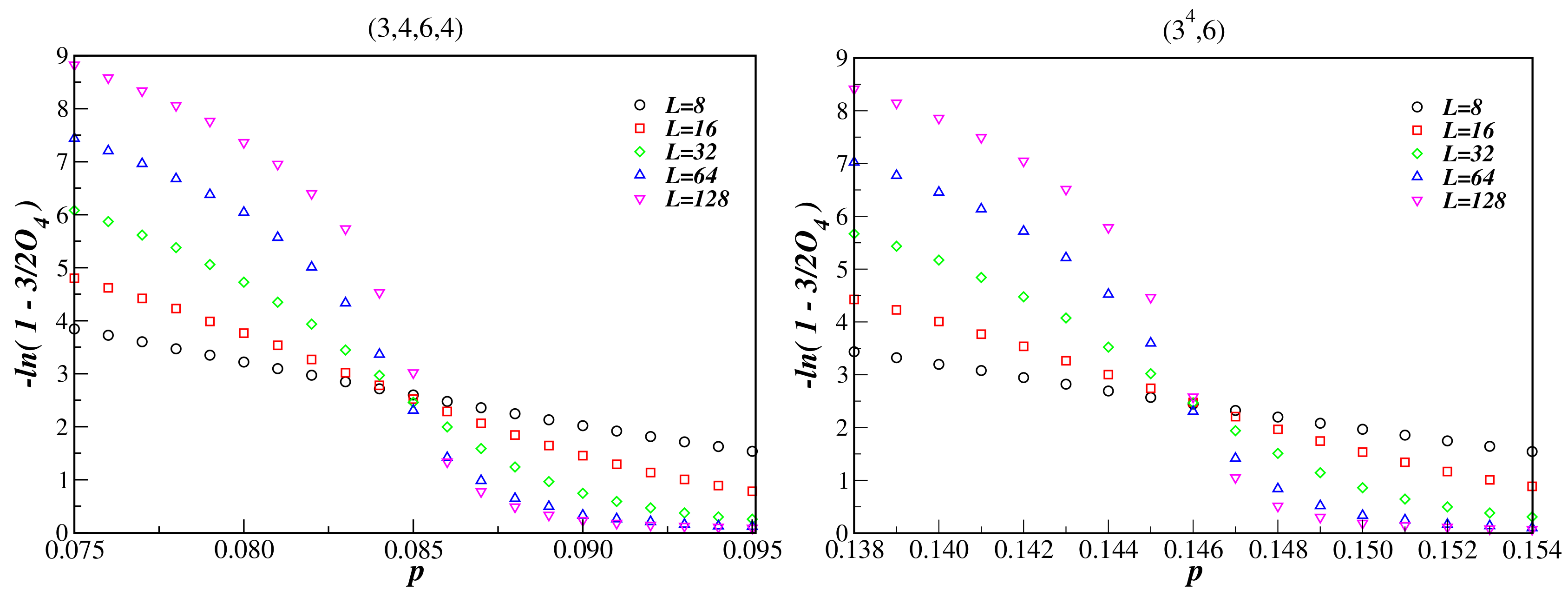
Figure 4.
Log–log plot of the dependence of the opinion on the linear system size L. Fitting data, we obtained the estimate for the critical ratio .
Figure 4.
Log–log plot of the dependence of the opinion on the linear system size L. Fitting data, we obtained the estimate for the critical ratio .

Figure 5.
Log–log plot of the at versus L for , and AL. Fitting data, we obtained the estimate for the critical ratio .
Figure 5.
Log–log plot of the at versus L for , and AL. Fitting data, we obtained the estimate for the critical ratio .

Figure 6.
at versus L for and , AL. Fitting data, we obtained another estimate for the critical ratio .
Figure 6.
at versus L for and , AL. Fitting data, we obtained another estimate for the critical ratio .
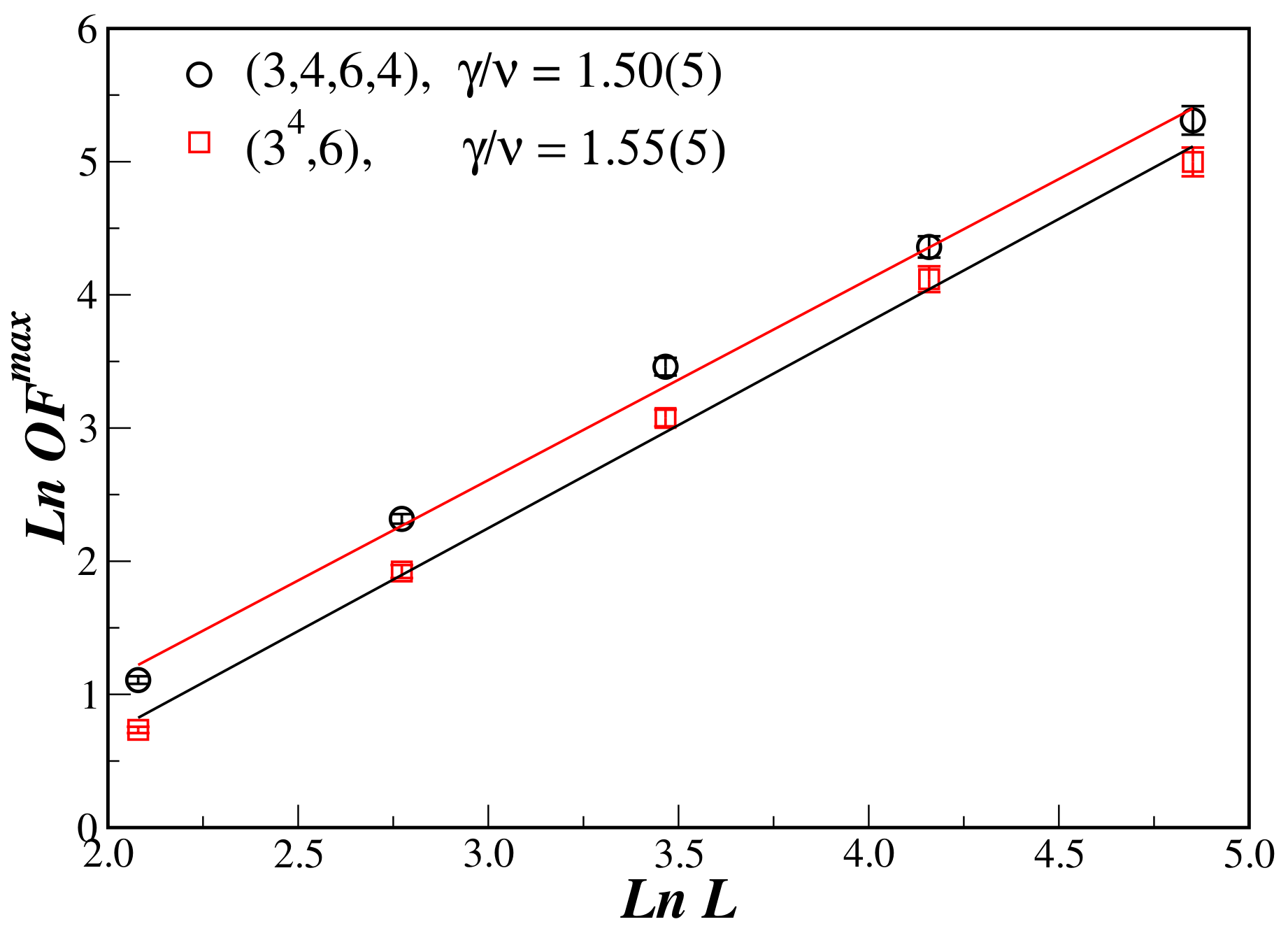
Figure 7.
Plot of versus the linear system size L for and AL. Fitting data, we obtained the estimate for the critical ratio .
Figure 7.
Plot of versus the linear system size L for and AL. Fitting data, we obtained the estimate for the critical ratio .

Figure 8.
(Color online) Data collapse of the opinion O, OF, and O4 shown in Figure 3 for , 64, and 128 (a–f) and (d–f) AL. The exponent ratios used here were , , and for , and , , and for AL.
Figure 8.
(Color online) Data collapse of the opinion O, OF, and O4 shown in Figure 3 for , 64, and 128 (a–f) and (d–f) AL. The exponent ratios used here were , , and for , and , , and for AL.


Table 1.
Critical parameter (), exponents, and effective dimension for majority vote model (MVM) on and [14]. For completeness, we cite data for Ising model on as well [18].
| MVM | Ising | ||
|---|---|---|---|
| 0.651(3) | 0.667(2) | ≈2.269 | |
| 0.603(9) | 0.608(4) | 0.61 | |
| 0.105(8) | 0.113(2) | 0.125 | |
| 1.48(11) | 1.60(4) | 1.75 | |
| 1.44(4) | 1.66(2) | 1.75 | |
| 1.16(5) | 0.84(6) | 1 | |
| . | 1.78(7) | 1.83(6) | 2 |
Table 2.
Critical parameter (), exponents, and effective dimension for continuous opinion dynamic (KCOD) model on and . For completeness, we cite data for KCOD model on as well [16].
Table 2.
Critical parameter (), exponents, and effective dimension for continuous opinion dynamic (KCOD) model on and . For completeness, we cite data for KCOD model on as well [16].
| KCOD | |||
|---|---|---|---|
| 0.085(6) | 0.146(5) | 0.2266(1) | |
| 0.605(9) | 0.606(4) | 0.559(1) | |
| 0.126(1) | 0.125(3) | 0.125(1) | |
| 1.50(7) | 1.54(6) | 1.75(1) | |
| 1.50(5) | 1.55(5) | ||
| 0.90(5) | 0.99(3) | 1.01(1) | |
| 1.75(6) | 1.80(7) |
© 2017 by the authors. Licensee MDPI, Basel, Switzerland. This article is an open access article distributed under the terms and conditions of the Creative Commons Attribution (CC BY) license (http://creativecommons.org/licenses/by/4.0/).
Share and Cite
MDPI and ACS Style
De Sousa Lima, F.W. The KCOD Model on (3,4,6,4) and (34,6) Archimedean Lattices. Entropy 2017, 19, 459. https://doi.org/10.3390/e19090459
AMA Style
De Sousa Lima FW. The KCOD Model on (3,4,6,4) and (34,6) Archimedean Lattices. Entropy. 2017; 19(9):459. https://doi.org/10.3390/e19090459
Chicago/Turabian StyleDe Sousa Lima, Francisco W. 2017. "The KCOD Model on (3,4,6,4) and (34,6) Archimedean Lattices" Entropy 19, no. 9: 459. https://doi.org/10.3390/e19090459
Note that from the first issue of 2016, this journal uses article numbers instead of page numbers. See further details here.