Automated Multiclass Classification of Spontaneous EEG Activity in Alzheimer’s Disease and Mild Cognitive Impairment

 ,
,  , , ,
, , ,
Abstract
:1. Introduction
2. Materials and Methods
2.1. Subjects
2.2. EEG Recording
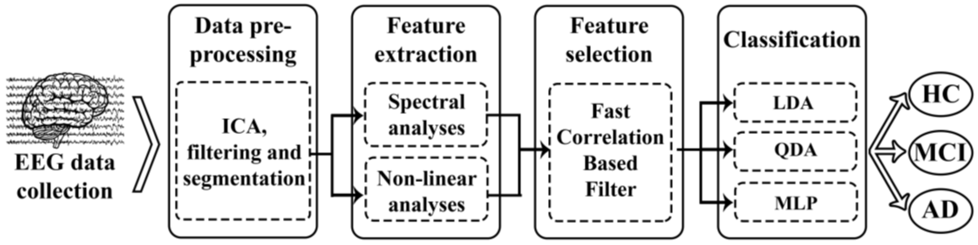
2.3. Methods
2.3.1. Feature Extraction
Spectral Analysis
- RP represents the relative contribution of different frequency components to the global power spectrum. RP is more appropriate than absolute power to analyze EEG data, as RP provides independent thresholds from the measurement equipment and lower inter-subject variability [27]. RP is obtained by summing the contribution of the desired spectral components:where and are the low and the high cut-off frequencies of each band, respectively.In this study, RP was calculated in the conventional EEG frequency bands: delta (δ, 1–4 Hz), theta (θ, 4–8 Hz), alpha (α, 8–13 Hz), beta-1 (β1, 13–19 Hz), beta-2 (β2, 19–30 Hz) and gamma (γ, 30–70 Hz).
- MF offers an alternative way to quantify the spectral changes of the EEG, and it is a simple index that summarizes the whole spectral content of the PSDn. MF is defined as the frequency that comprises 50% of the PSDn power:Previous studies suggested that MF provides a better performance for the characterization of brain activity than mean frequency, whose original definition is based on the computation of the spectral centroid [28].
- IAF evaluates the frequency at which the maximum alpha power is reached. Alpha oscillations are dominant in the EEG of resting normal subjects, with the exception of irregular activity in the delta band and lower frequencies. This issue involves that the PSD displays a peak around the alpha band. The IAF estimation in the present work is based on the calculation of the MF in the extended alpha band (4–15 Hz), as previous EEG studies on AD recommended [29]. This is shown in the following equation:
- SE estimates the signal irregularity in terms of the flatness of the power spectrum [30]. On the one hand, a uniform power spectrum with a broad spectral content (e.g., a highly irregular signal like white noise) provides a high entropy value. On the other hand, a narrow power spectrum with only a few spectral components (e.g., a highly predictable signal like a sum of sinusoids) yields a low SE value. The equation for calculating SE would be:
Nonlinear Analysis
- LZC estimates the complexity of a finite sequence of symbols. LZC analysis is based on a coarse-graining of measurements. Therefore, the EEG signal must be previously transformed into a finite symbol string. In this study, we used the simplest possible way: a binary sequence conversion (zeros and ones). By comparison with a threshold Td, the original signal samples are converted into a 0–1 sequence with defined by:The threshold Td is estimated as the median value of the signals amplitude in each channel because it is more robust to outliers. The string P is then scanned from left to right and a complexity counter is increased by one every time a new subsequence of consecutive characters is encountered in the scanning process. In order to obtain a complexity measure that is independent of the sequence length, should be normalized. For a binary conversion, the upper bound of is given by and can be normalized via :LZC values are normalized between 0 and 1, with higher LZC values for more complex time series. The detailed algorithm for LZC measure can be found in [35].
- CTM quantifies the variability of a given time series on the basis of its first-order differences. For CTM calculation, scatter plots of first differences of the data are drawn. The value of CTM is computed as the proportion of points in the plot that fall within a radius ρ, which must be specified [36]. For a time series with N samples, would be the total number of points in the scatter plot that can be plotted by representing versus . Subsequently, the CTM of the time series can be computed as:whereThus, CTM ranges between 0 and 1, with higher values corresponding to points more concentrated around the center of the plot (i.e., corresponding to less degree of variability).
- SampEn is an embedding entropy used to quantify the irregularity. It can be applied to short and relatively noisy time series [37]. To compute SampEn, two input parameters should be specified: a run length m and a tolerance window r. SampEn is the negative natural logarithm of the conditional probability that two sequences similar for m points remain similar at the next point, within a tolerance r, excluding self-matches [37]. Thus, SampEn assigns a nonnegative number to a time series, with larger values corresponding to greater signal irregularity. For a time series of N points, , the vectors of length m are formed as . The distances among vectors are calculated as the maximum absolute distance between their corresponding scalar elements. is the number of vectors that satisfy the condition that their distance is less than r. The counting number of different vectors is calculated and normalized as [37]:Repeating the process for vectors of length m + 1, can be obtained and SampEn can be defined as:
- FuzzyEn provides information about how a signal fluctuates with time by comparing the time series with a delayed version of itself [38]. As SampEn, higher FuzzyEn values are associated with more irregular time series. To compute FuzzyEn, three parameters must be fixed. The first parameter, m, is the length of the vectors to be compared, like in SampEn. The other ones, r and n, are the width and the gradient of the boundary of the exponential function, respectively [38]. Given a time series the FuzzyEn algorithm reads as follows:
- Compose N − m + 1 vectors of length m such that:where is given by:
- Compute the distance, , between each two vectors, and , as the maximum absolute difference of their corresponding scalar components. Given n and r, calculate the similarity degree, , between and through a fuzzy function :
- Define the function as:
- Increase the dimension to m + 1, form the vector and the function . Finally, FuzzyEn(m, n, r) is defined as the negative natural logarithm of the deviation of from :
- AMI is the particularization of mutual information applied to time-delayed versions of the same sequence. Mutual information is a metric derived from Shannon’s information theory to estimate the information gain from observations of one random event on another [31]. AMI estimates, on average, the degree to which a time-delayed version of a signal can be predicted from the original one. Thus, more predictable time series, and accordingly more regular, lead to higher AMI values. The AMI between and is [31]:where is the probability density for the measurement , while is the joint probability density for the measurements of and . In this study, the AMI was estimated over a time delay from 0 to 0.5 s and was then normalized, so that AMI.
2.3.2. Feature Selection: Fast-Correlation-Based Filter
- In the first step, a relevance analysis of the features is done. Thus, SU between each feature Xi and the group membership Y is computed as follows:where H(·) is the well-known Shannon’s entropy, H(Xi|Y) is the Shannon’s entropy of Xi conditioned on Y, and I is the number of features extracted (in our study, I = 14 features). SU is normalized to the range [0, 1], with a value of SU = 1, indicating that, when knowing one feature, it is possible to completely predict the other, and a value of SU = 0 indicates that the two variables are independent. Then, a ranking of features is done based on their relevance since the higher the value of SU is, the more relevant the feature is.
- The second step is a redundancy analysis used to discard redundant features. SU between each pair of features SU(Xi, Xj) is sequentially estimated beginning from the first-ranked ones. If Xi shares more information with Xj than with the corresponding group Y, SU(Xi, Xj) SU(Xi, Y) (with Xi being more highly ranked than Xj), the feature j is discarded due to redundancy and it is not considered in subsequent comparisons. The optimal features are those not discarded when the algorithm ends.
2.3.3. Classification Approach
Linear and Quadratic Discriminant Analysis (LDA and QDA)
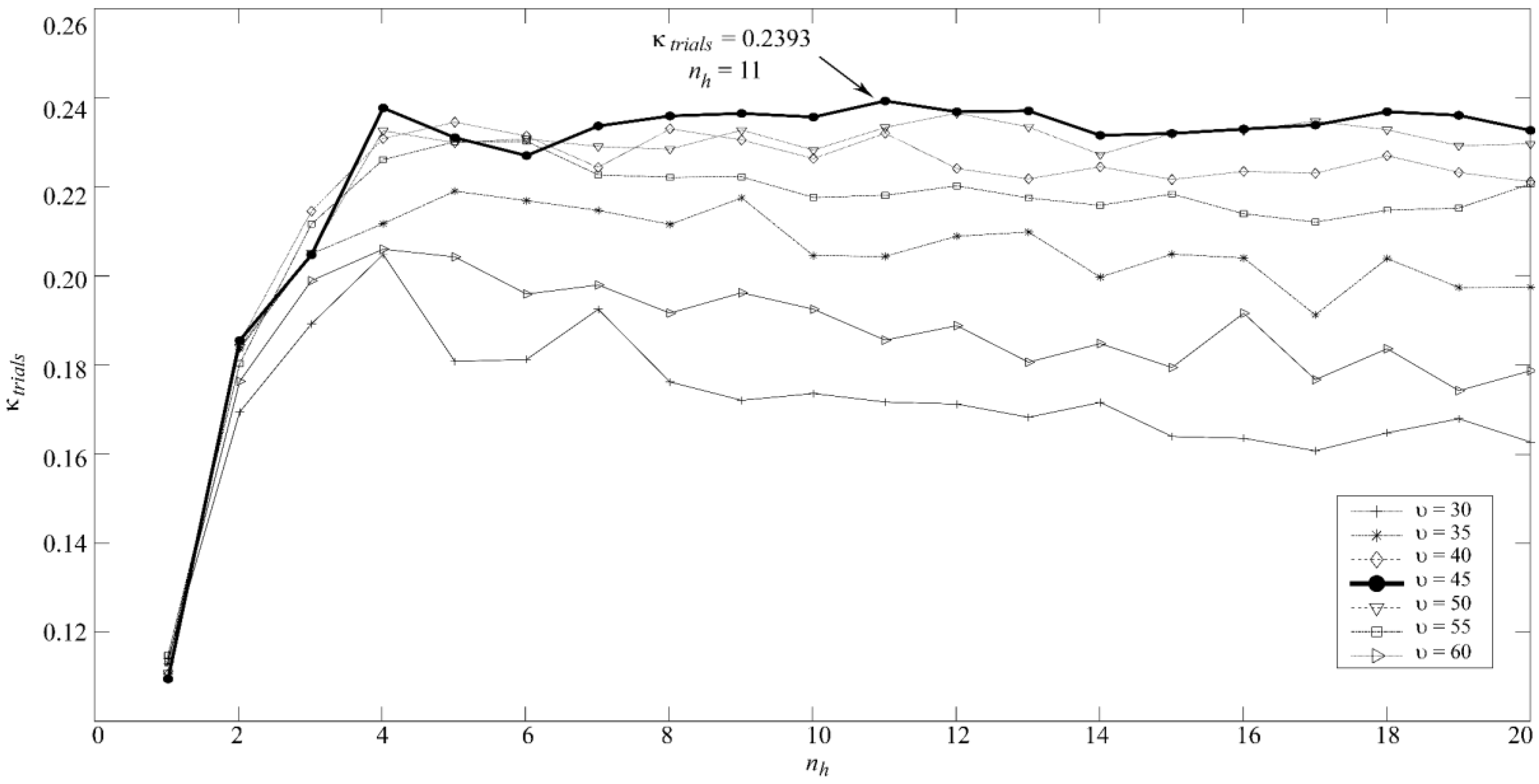
Multi-Layer Perceptron Artificial Neural Network (MLP)
2.4. Statistical Analysis
3. Results
3.1. Training Set
3.2. Test Set
4. Discussion
4.1. Spectral and Nonlinear Characterization of AD and MCI
4.2. Towards a Screening Protocol of AD
- If the MLP model predicts AD, recommend beginning a treatment since most probably (89.47%, 17 out of 19 subjects) the patient suffers from AD or MCI.
- If the MLP model predicts HC, do not treat the patient, since most probably (88.89%, 16 out of 18 subjects) he/she does not suffer from AD; consider a regular evaluation of the subject in the persistence of symptoms in order to minimize the number of AD and MCI missed subjects.
- If the MLP predicts MCI, conduct a regular evaluation of the patient since doubts arise about the cognitive status of the subject.
4.3. Limitations and Future Research Lines
5. Conclusions
Acknowledgments
Author Contributions
Conflicts of Interest
References
- Alzheimer’s Association. 2017 Alzheimer’s disease facts and figures. Alzheimer’s Dement. 2017, 13, 325–373. [Google Scholar] [CrossRef]
- Petersen, R.C. Alzheimer’s disease: Progress in prediction. Lancet Neurol. 2010, 9, 4–5. [Google Scholar] [CrossRef]
- Mufson, E.J.; Binder, L.; Counts, S.E.; DeKosky, S.T.; DeToledo-Morrell, L.; Ginsberg, S.D.; Ikonomovic, M.D.; Perez, S.E.; Scheff, S.W. Mild cognitive impairment: Pathology and mechanisms. Acta Neuropathol. 2012, 123, 13–30. [Google Scholar] [CrossRef] [PubMed]
- Davatzikos, C.; Bhatt, P.; Shaw, L.M.; Batmanghelich, K.N.; Trojanowski, J.Q. Prediction of MCI to AD conversion, via MRI, CSF biomarkers, and pattern classification. Neurobiol. Aging 2011, 32. [Google Scholar] [CrossRef] [PubMed]
- Lin, P.-J.; Neumann, P.J. The economics of mild cognitive impairment. Alzheimers Dement. 2013, 9, 58–62. [Google Scholar] [CrossRef] [PubMed]
- Ewers, M.; Sperling, R.A.; Klunk, W.E.; Weiner, M.W.; Hampel, H. Neuroimaging markers for the prediction and early diagnosis of Alzheimer’s disease dementia. Trends Neurosci. 2011, 34, 430–442. [Google Scholar] [CrossRef] [PubMed]
- Poza, J.; Gómez, C.; García, M.; Corralejo, R.; Fernández, A.; Hornero, R. Analysis of neural dynamics in mild cognitive impairment and Alzheimer’s disease using wavelet turbulence. J. Neural Eng. 2014, 11, 26010. [Google Scholar] [CrossRef] [PubMed]
- Fernández, A.; Hornero, R.; Gómez, C.; Turrero, A.; Gil-Gregorio, P.; Matías-Santos, J.; Ortiz, T. Complexity analysis of spontaneous brain activity in Alzheimer disease and mild cognitive impairment: An MEG study. Alzheimer Dis. Assoc. Disord. 2010, 24, 182–189. [Google Scholar] [CrossRef] [PubMed]
- Hornero, R.; Abasolo, D.; Escudero, J.; Gomez, C. Nonlinear analysis of electroencephalogram and magnetoencephalogram recordings in patients with Alzheimer’s disease. Philos. Trans. R. Soc. A Math. Phys. Eng. Sci. 2009, 367, 317–336. [Google Scholar] [CrossRef] [PubMed] [Green Version]
- Stam, C.J. Nonlinear dynamical analysis of EEG and MEG: Review of an emerging field. Clin. Neurophysiol. 2005, 116, 2266–2301. [Google Scholar] [CrossRef] [PubMed]
- Woon, W.L.; Cichocki, A.; Vialatte, F.; Musha, T. Techniques for early detection of Alzheimer’s disease using spontaneous EEG recordings. Physiol. Meas. 2007, 28, 335–347. [Google Scholar] [CrossRef] [PubMed]
- Abásolo, D.; Hornero, R.; Gómez, C.; García, M.; López, M. Analysis of EEG background activity in Alzheimer’s disease patients with Lempel–Ziv complexity and central tendency measure. Med. Eng. Phys. 2006, 28, 315–322. [Google Scholar] [CrossRef] [PubMed] [Green Version]
- Gasser, U.S.; Rousson, V.; Hentschel, F.; Sattel, H.; Gasser, T. Alzheimer disease versus mixed dementias: An EEG perspective. Clin. Neurophysiol. 2008, 119, 2255–2259. [Google Scholar] [CrossRef] [PubMed]
- Baker, M.; Akrofi, K.; Schiffer, R.; Boyle, M.W.O. EEG Patterns in Mild Cognitive Impairment (MCI) Patients. Open Neuroimag. J. 2008, 2, 52–55. [Google Scholar] [CrossRef] [PubMed]
- Yu, L.; Liu, H. Efficient Feature Selection via Analysis of Relevance and Redundancy. J. Mach. Learn. Res. 2004, 5, 1205–1224. [Google Scholar] [CrossRef]
- Bertè, F.; Lamponi, G.; Calabrò, R.S.; Bramanti, P. Elman neural network for the early identification of cognitive impairment in Alzheimer’s disease. Funct. Neurol. 2014, 29, 57–65. [Google Scholar] [PubMed]
- Buscema, M.; Vernieri, F.; Massini, G.; Scrascia, F.; Breda, M.; Rossini, P.M.; Grossi, E. An improved I-FAST system for the diagnosis of Alzheimer’s disease from unprocessed electroencephalograms by using robust invariant features. Artif. Intell. Med. 2015, 64, 59–74. [Google Scholar] [CrossRef] [PubMed]
- Huang, C.; Wahlund, L.-O.; Dierks, T.; Julin, P.; Winblad, B.; Jelic, V. Discrimination of Alzheimer’s disease and mild cognitive impairment by equivalent EEG sources: A cross-sectional and longitudinal study. Clin. Neurophysiol. 2000, 111, 1961–1967. [Google Scholar] [CrossRef]
- Iqbal, K.; Alonso, A.D.C.; Chen, S.; Chohan, M.O.; El-Akkad, E.; Gong, C.-X.; Khatoon, S.; Li, B.; Liu, F.; Rahman, A.; et al. Tau pathology in Alzheimer disease and other tauopathies. Biochim. Biophys. Acta Mol. Basis Dis. 2005, 1739, 198–210. [Google Scholar] [CrossRef] [PubMed]
- Poza, J.; Gómez, C.; García, M.; Tola-Arribas, M.A.; Carreres, A.; Cano, M.; Hornero, R. Spatio-Temporal Fluctuations of Neural Dynamics in Mild Cognitive Impairment and Alzheimer’s Disease. Curr. Alzheimer Res. 2017, 14, 924–936. [Google Scholar] [CrossRef] [PubMed]
- McBride, J.C.; Zhao, X.; Munro, N.B.; Smith, C.D.; Jicha, G.A.; Hively, L.; Broster, L.S.; Schmitt, F.A.; Kryscio, R.J.; Jiang, Y. Spectral and complexity analysis of scalp EEG characteristics for mild cognitive impairment and early Alzheimer’s disease. Comput. Methods Programs Biomed. 2014, 114, 153–163. [Google Scholar] [CrossRef] [PubMed]
- Petrosian, A.A.; Prokhorov, D.V.; Lajara-Nanson, W.; Schiffer, R.B. Recurrent neural network-based approach for early recognition of Alzheimer’s disease in EEG. Clin. Neurophysiol. 2001, 112, 1378–1387. [Google Scholar] [CrossRef]
- Albert, M.S.; DeKosky, S.T.; Dickson, D.; Dubois, B.; Feldman, H.H.; Fox, N.C.; Gamst, A.; Holtzman, D.M.; Jagust, W.J.; Petersen, R.C.; et al. The diagnosis of mild cognitive impairment due to Alzheimer’s disease: Recommendations from the National Institute on Aging-Alzheimer’s Association workgroups on diagnostic guidelines for Alzheimer’s disease. Alzheimer’s Dement. 2011, 7, 270–279. [Google Scholar] [CrossRef] [PubMed]
- Jeong, J. EEG dynamics in patients with Alzheimer’s disease. Clin. Neurophysiol. 2004, 115, 1490–1505. [Google Scholar] [CrossRef] [PubMed]
- Dauwels, J.; Vialatte, F.-B.; Cichocki, A. Diagnosis of alzheimers disease from eeg signals: Where are we standing? Curr. Alzheimer Res. 2010, 7, 1–43. [Google Scholar] [CrossRef]
- Osipova, D.; Ahveninen, J.; Kaakkola, S.; Jääskeläinen, I.P.; Huttunen, J.; Pekkonen, E. Effects of scopolamine on MEG spectral power and coherence in elderly subjects. Clin. Neurophysiol. 2003, 114, 1902–1907. [Google Scholar] [CrossRef]
- Rodriguez, G.; Copello, F.; Vitali, P.; Perego, G.; Nobili, F. EEG spectral profile to stage Alzheimer’s disease. Clin. Neurophysiol. 1999, 110, 1831–1837. [Google Scholar] [CrossRef]
- Poza, J.; Hornero, R.; Abásolo, D.; Fernández, A.; García, M. Extraction of spectral based measures from MEG background oscillations in Alzheimer’s disease. Med. Eng. Phys. 2007, 29, 1073–1083. [Google Scholar] [CrossRef] [PubMed] [Green Version]
- Moretti, D.V.; Babiloni, C.; Binetti, G.; Cassetta, E.; Dal Forno, G.; Ferreric, F.; Ferri, R.; Lanuzza, B.; Miniussi, C.; Nobili, F.; et al. Individual analysis of EEG frequency and band power in mild Alzheimer’s disease. Clin. Neurophysiol. 2004, 115, 299–308. [Google Scholar] [CrossRef]
- Powell, G.E.; Percival, I.C. A spectral entropy method for distinguishing regular and irregular motion of Hamiltonian systems. J. Phys. A Math. Gen. 1979, 12, 2053–2071. [Google Scholar] [CrossRef]
- Abásolo, D.; Escudero, J.; Hornero, R.; Gómez, C.; Espino, P. Approximate entropy and auto mutual information analysis of the electroencephalogram in Alzheimer’s disease patients. Med. Biol. Eng. Comput. 2008, 46, 1019–1028. [Google Scholar] [CrossRef] [PubMed] [Green Version]
- Gómez, C.; Hornero, R.; Abásolo, D.; Fernández, A.; Escudero, J. Analysis of the magnetoencephalogram background activity in Alzheimer’s disease patients with auto-mutual information. Comput. Methods Programs Biomed. 2007, 87, 239–247. [Google Scholar] [CrossRef] [PubMed] [Green Version]
- Jeong, J.; Gore, J.C.; Peterson, B.S. Mutual information analysis of the EEG in patients with Alzheimer’s disease. Clin. Neurophysiol. 2001, 112, 827–835. [Google Scholar] [CrossRef]
- Cao, Y.; Cai, L.; Wang, J.; Wang, R.; Yu, H.; Cao, Y.; Liu, J. Characterization of complexity in the electroencephalograph activity of Alzheimer’s disease based on fuzzy entropy. Chaos 2015, 25, 83116. [Google Scholar] [CrossRef] [PubMed]
- Lempel, A.; Ziv, J. On the complexity of finite sequences. IEEE Trans. Inf. Theory 1976, 22, 75–81. [Google Scholar] [CrossRef]
- Cohen, M.E.; Hudson, D.L.; Deedwania, P.C. Applying continuous chaotic modeling to cardiac signal analysis. IEEE Eng. Med. Biol. Mag. 1996, 15, 97–102. [Google Scholar] [CrossRef]
- Ben-Mizrachi, A.; Procaccia, I.; Grassberger, P. Characterization of experimental (noisy) strange attractors. Phys. Rev. A 1984, 29, 975–977. [Google Scholar] [CrossRef]
- Monge, J.; Gómez, C.; Poza, J.; Fernández, A.; Quintero, J.; Hornero, R. MEG analysis of neural dynamics in attention-deficit/hyperactivity disorder with fuzzy entropy. Med. Eng. Phys. 2015, 37, 416–423. [Google Scholar] [CrossRef] [PubMed]
- Bishop, C.M. Neural Networks for Pattern Recognition; Oxford University Press: Oxford, UK, 1995; ISBN 9780198538646. [Google Scholar]
- Bishop, C.M. Pattern Recognition and Machine Learning. J. Electron. Imaging 2007, 16, 49901. [Google Scholar] [CrossRef]
- Zhang, G.P. Neural networks for classification: A survey. IEEE Trans. Syst. Man Cybern. Part C Appl. Rev. 2000, 30, 451–462. [Google Scholar] [CrossRef]
- Hornik, K. Approximation capabilities of multilayer feedforward networks. Neural Netw. 1991, 4, 251–257. [Google Scholar] [CrossRef]
- Gutiérrez-Tobal, G.C.; Álvarez, D.; Marcos, J.V.; Del Campo, F.; Hornero, R. Pattern recognition in airflow recordings to assist in the sleep apnoea-hypopnoea syndrome diagnosis. Med. Biol. Eng. Comput. 2013, 51, 1367–1380. [Google Scholar] [CrossRef] [PubMed]
- Nabney, I.T. NETLAB: Algorithms for Pattern Recognition; Springer Science & Business Media: New York, NY, USA, 2002. [Google Scholar]
- Witten, I.H.; Frank, E.; Hall, M.A. Data Mining: Practical Machine Learning Tools and Techniques; Morgan Kaufmann Publishers: Burlington, ON, Canada, 2011; ISBN 0080890369. [Google Scholar]
- Richman, J.S.; Moorman, J.R. Physiological time-series analysis using approximate entropy and sample entropy. Am. J. Physiol. Heart Circ. Physiol. 2000, 278, 2039–2049. [Google Scholar] [CrossRef] [PubMed]
- Baraniuk, R.G.; Flandrin, P.; Janssen, A.J.E.M.; Michel, O.J.J. Measuring time-frequency information content using the Reényi entropies. IEEE Trans. Inf. Theory 2001, 47, 1391–1409. [Google Scholar] [CrossRef]

| Training Set | Test Set | |||||
|---|---|---|---|---|---|---|
| HC | MCI | AD | HC | MCI | AD | |
| Number of subjects | 20 | 20 | 20 | 17 | 17 | 17 |
| Number of trials | 912 | 937 | 917 | 752 | 847 | 757 |
| Age (years) | 75.6 | 77.9 | 80.7 | 76.4 | 75.3 | 82.4 |
| (median [IQR]) | [74.1, 77.6] | [67.9, 79.8] | [74.7, 83.3] | [73.6, 78.9] | [69.8, 82.0] | [77.7, 83.9] |
| Gender (Male:Female) | 8:12 | 8:12 | 5:15 | 4:13 | 8:9 | 7:10 |
| MMSE 1 | 29 | 27.5 | 21 | 29 | 27 | 22 |
| (median [IQR]) | [28, 30] | [26.5, 29] | [18.5, 22.5] | [28, 30] | [27, 28] | [20, 24] |
| B-ADL 2 | 1.1 | 2.9 | 5.8 | 1.2 | 2.8 | 6.4 |
| (median [IQR]) | [1.0, 1.2] | [2.4, 3.3] | [5.1, 7.2] | [1.0, 1.3] | [2.3, 2.5] | [5.0, 4.3] |
| Education level (A:B) 3 | 5:15 | 11:9 | 8:12 | 5:12 | 12:5 | 10:7 |
| Features | HC | MCI | AD |
|---|---|---|---|
| RP(δ) | 0.227 [0.179, 0.277] | 0.164 [0.102, 0.221] | 0.158 [0.103, 0.229] |
| RP(θ) | 0.111 [0.083, 0.131] | 0.122 [0.087, 0.155] | 0.143 [0.103, 0.188] |
| RP(α) | 0.243 [0.174, 0.291] | 0.317 [0.224, 0.544] | 0.279 [0.192, 0.447] |
| RP(β1) | 0.128 [0.101, 0.155] | 0.101 [0.081, 0.160] | 0.101 [0.073, 0.141] |
| RP(β2) | 0.111 [0.084, 0.138] | 0.105 [0.048, 0.135] | 0.091 [0.060, 0.119] |
| RP(γ) | 0.097 [0.074, 0.168] | 0.087 [0.037, 0.145] | 0.089 [0.047, 0.141] |
| MF | 10.584 [9.690, 11.900] | 10.467 [8.639, 12.285] | 9.971 [9.030, 10.997] |
| IAF | 9.502 [8.751, 9.996] | 9.404 [8.519, 9.972] | 8.811 [8.510, 9.474] |
| SE | 0.813 [0.760, 0.822] | 0.796 [0.695, 0.816] | 0.782 [0.733, 0.809] |
| LZC | 0.684 [0.6331, 0.7360] | 0.667 [0.551, 0.731] | 0.663 [0.589, 0.713] |
| CTM | 0.101 [0.076, 0.129] | 0.111 [0.086, 0.165] | 0.116 [0.077, 0.183] |
| SampEn | 1.366 [1.288, 1.540] | 1.312 [1.103, 1.489] | 1.274 [1.034, 1.489] |
| FuzzyEn | 0.532 [0.466, 0.624] | 0.514 [0.395, 0.618] | 0.508 [0.427, 0.584] |
| AMI | −0.149 [−0.184, −0.130] | −0.149 [−0.175, −0.124] | −0.145 [−0.164, −0.128] |
| LDA | QDA | MLP | |||||||
|---|---|---|---|---|---|---|---|---|---|
| Actual ↓\Estimated → | HC | MCI | AD | HC | MCI | AD | HC | MCI | AD |
| HC | 11 | 4 | 2 | 13 | 3 | 1 | 12 | 3 | 2 |
| MCI | 4 | 7 | 6 | 4 | 7 | 6 | 4 | 8 | 5 |
| AD | 2 | 3 | 12 | 3 | 3 | 11 | 2 | 3 | 12 |
| HC vs. All | AD vs. All | |||||
|---|---|---|---|---|---|---|
| LDA | QDA | MLP | LDA | QDA | MLP | |
| Se (%) | 82.35 | 79.41 | 82.35 | 70.59 | 64.71 | 70.59 |
| Sp (%) | 64.71 | 76.47 | 70.59 | 76.47 | 79.41 | 79.41 |
| Acc (%) | 76.47 | 78.43 | 78.43 | 74.51 | 74.51 | 76.47 |
| PPV (%) | 82.35 | 87.10 | 84.85 | 60.00 | 61.11 | 63.16 |
| NPV (%) | 64.71 | 65.00 | 66.67 | 83.87 | 81.82 | 84.38 |
© 2018 by the authors. Licensee MDPI, Basel, Switzerland. This article is an open access article distributed under the terms and conditions of the Creative Commons Attribution (CC BY) license (http://creativecommons.org/licenses/by/4.0/).
Share and Cite
Ruiz-Gómez, S.J.; Gómez, C.; Poza, J.; Gutiérrez-Tobal, G.C.; Tola-Arribas, M.A.; Cano, M.; Hornero, R. Automated Multiclass Classification of Spontaneous EEG Activity in Alzheimer’s Disease and Mild Cognitive Impairment. Entropy 2018, 20, 35. https://doi.org/10.3390/e20010035
Ruiz-Gómez SJ, Gómez C, Poza J, Gutiérrez-Tobal GC, Tola-Arribas MA, Cano M, Hornero R. Automated Multiclass Classification of Spontaneous EEG Activity in Alzheimer’s Disease and Mild Cognitive Impairment. Entropy. 2018; 20(1):35. https://doi.org/10.3390/e20010035
Chicago/Turabian StyleRuiz-Gómez, Saúl J., Carlos Gómez, Jesús Poza, Gonzalo C. Gutiérrez-Tobal, Miguel A. Tola-Arribas, Mónica Cano, and Roberto Hornero. 2018. "Automated Multiclass Classification of Spontaneous EEG Activity in Alzheimer’s Disease and Mild Cognitive Impairment" Entropy 20, no. 1: 35. https://doi.org/10.3390/e20010035