Computational Information Geometry for Binary Classification of High-Dimensional Random Tensors ^†

Abstract

Evaluating the performance of Bayesian classification in a high-dimensional random tensor is a fundamental problem, usually difficult and under-studied. In this work, we consider two Signal to Noise Ratio (SNR)-based binary classification problems of interest. Under the alternative hypothesis, i.e., for a non-zero SNR, the observed signals are either a noisy rank-R tensor admitting a Q-order Canonical Polyadic Decomposition (CPD) with large factors of size $N_q\times R$, i.e., for $1\le q\le Q$, where $R,N_q\to \infty$ with $R^{1/q}/N_q$ converge towards a finite constant or a noisy tensor admitting TucKer Decomposition (TKD) of multilinear $(M_1,\dots ,M_Q)$-rank with large factors of size $N_q\times M_q$, i.e., for $1\le q\le Q$, where $N_q,M_q\to \infty$ with $M_q/N_q$ converge towards a finite constant. The classification of the random entries (coefficients) of the core tensor in the CPD/TKD is hard to study since the exact derivation of the minimal Bayes’ error probability is mathematically intractable. To circumvent this difficulty, the Chernoff Upper Bound (CUB) for larger SNR and the Fisher information at low SNR are derived and studied, based on information geometry theory. The tightest CUB is reached for the value minimizing the error exponent, denoted by $s^{\star }$. In general, due to the asymmetry of the s-divergence, the Bhattacharyya Upper Bound (BUB) (that is, the Chernoff Information calculated at $s^{\star }=1/2$) cannot solve this problem effectively. As a consequence, we rely on a costly numerical optimization strategy to find $s^{\star }$. However, thanks to powerful random matrix theory tools, a simple analytical expression of $s^{\star }$ is provided with respect to the Signal to Noise Ratio (SNR) in the two schemes considered. This work shows that the BUB is the tightest bound at low SNRs. However, for higher SNRs, the latest property is no longer true.

1. Introduction

1.1. State-of-the-Art and Problem Statement

Evaluating the performance limit for the “Gaussian information plus noise” binary classification problem is a challenging research topic, see for instance [1,2,3,4,5,6,7]. Given a binary hypothesis problem, the Bayes’ decision rule is based on the principle of the largest posterior probability. Specifically, the Bayesian detector chooses the alternative hypothesis ${\mathcal{H}}_1$ if $\mathrm{Pr}\left({\mathcal{H}}_1\right|\mathbf{y})>\mathrm{Pr}\left({\mathcal{H}}_0\right|\mathbf{y})$ for a given N-dimensional measurement vector $\mathbf{y}$ or the null hypothesis ${\mathcal{H}}_0$, otherwise. Consequently, the optimal decision rule can often only be derived at the price of a costly numerical computation of the log posterior-odds ratio [3] since an exact calculation of the minimal Bayes’ error probability $P_e^{\left(N\right)}$ is often intractable [3,8]. To circumvent this problem, it is standard to exploit well-known bounds on $P_e^{\left(N\right)}$ based on information theory [9,10,11,12,13]. In particular, the Chernoff information [14,15] is asymptotically (in N) relied on the exponential rate of $P_e^{\left(N\right)}$. It turns out that the Chernoff information is very useful in many practically important problems as for instance, distributed sparse detection [16], sparse support recovery [17], energy detection [18], multi-input and multi-output (MIMO) radar processing [19,20], network secrecy [21], angular resolution limit in array processing [22], detection performance for informed communication systems [23], just to name a few. In addition, the Chernoff information bound can be tight for a minimal s-divergence over parameter $s\in (0,1)$. Generally, this step requires solving numerically an optimization problem [24] and often leads to a complicated and uninformative expression of the optimal value of s. To circumvent this difficulty, a simplified case of $s=1/2$ is often used corresponding to the well-known Bhattacharyya divergence [13] at the price of a less accurate prediction of $P_e^{\left(N\right)}$. In information geometry, parameter s is often called $\alpha$, and the s-divergence is the so-called Chernoff $\alpha$-divergence [24].

The tensor decomposition theory is a timely and prominent research topic [25,26]. Confronting the problem of extracting useful information from a massive and multidimentional volume of measurements, it is shown that tensors are extremely relevant. In the standard literature, two main families of tensor decomposition are prominent, namely the Canonical Polyadic Decomposition (CPD) [26] and the Tucker decomposition (TKD)/HOSVD (High-Order SVD) [27,28]. These approaches are two possible multilinear generalization of the Singular Value Decomposition (SVD). A natural generalization to tensors of the usual concept of rank for matrices is called the CPD. The tensorial/canonical rank of a P-order tensor is equal to the minimal positive integer, say R, of unit rank tensors that must be summed up for perfect recovery. A unit rank tensor is the outer product of P vectors. In addition, the CPD has remarkable uniqueness properties [26] and involves only a reduced number of free parameters due to the constraint of minimality on R. Unfortunately, unlike the matrix case, the set of tensors with fixed (tensorial) rank is not close [29,30]. This singularity implies that the problem of the computation of the CPD is mathematically ill-posed. The consequence is that its numerical computation remains non trivial and is usually done using suboptimal iterative algorithms [31]. Note that this problem can sometimes be avoided by exploiting some natural hidden structures in the physical model [32]. The TKD [28] and the HOSVD [27] are two popular decompositions being an alternative to the CPD. Under this circumstance, alternative definition of rank is required, since the tensorial rank based on CPD scenario is no longer appropriate. In particular, stardard definition of multilinear rank defined as the set of positive integers $\{R_1,\dots ,R_P\}$ where each integer, $R_p$, is the usual rank of the p-th mode. Following the Eckart-Young theorem at each mode level [33], this construction is non-iterative, optimal and practical. In real-time computation [34] or adaptively computation [35], it is shown that this approach is suitable. However, in general, the low (multilinear) rank tensor based on this procedure is suboptimal [27]. More precisely, for tensors of order strictly greater than two, a generalization of the Eckart-Young theorem does not exist.

The classification performance of a multilinear tensor following the CPD and TKD can be derived and studied. It is interesting to note that the classification theory for tensors is very under studied. Based on our knowledge on the topic, only the publication [36] tackles this problem in the context of radar multidimensional data detection. A major difference with this publication is that their analysis is based on the performance of a low rank detection after matched filtering.

More precisely, we consider two cases where the observations are either (1) a noisy rank-R tensor admitting a Q-order CPD with large factors of size $N_q\times R$, i.e., for $1\le q\le Q$, $R,N_q\to \infty$ with $R^{1/q}/N_q$ converging towards a finite constant, or (2) a noisy tensor admitting a TKD of multilinear $(M_1,\dots ,M_Q)$-rank with large factors of size $N_q\times M_q$, i.e., for $1\le q\le Q$, where $N_q,M_q\to \infty$ with $M_q/N_q$ converging towards a finite constant. A standard approach for zero-mean independent Gaussian core and noise tensors, is to define the Signal to Noise Ratio by $\mathrm{SNR}={\sigma }_{\mathbf{s}}^2/{\sigma }^2$ where ${\sigma }_{\mathbf{s}}^2$ and ${\sigma }^2$ are the variances of the vectorized core and noise tensors, respectively. So, the binary classification can be described in the following way:

Under the null hypothesis ${\mathcal{H}}_0$, $\mathrm{SNR}=0$, meaning that the observed tensor contains only noise. Conversely, the alternative hypothesis ${\mathcal{H}}_1$ is based on $\mathrm{SNR}\ne 0$, meaning that there exists a multilinear signal of interest. First note that there exists a lack of contribution dealing with classification performance for tensors. Since the exact derivation of the error probability is intractable, the performance of the classification of the core tensor random entries is hard to evaluate. To circumvent this audible difficulty, based on computational information geometry theory, we consider the Chernoff Upper Bound (CUB), and the Fisher information in the context of massive measurement vectors. The error exponent can be minimized at $s^{\star }$, which corresponds to the reachable tightest CUB. In general, due to the asymmetry of the s-divergence, the Bhattacharyya Upper Bound (BUB)—Chernoff Information calculated at $s^{\star }=1/2$—cannot solve this problem effectively. As a consequence, we rely on a costly numerical optimization strategy to find $s^{\star }$. However, with respect to different Signal to Noise Ratios (SNR), we provide simple analytical expressions of $s^{\star }$, thanks to the so-called Random Matrix Theory (RMT). For low SNR, analytical expressions of the Fisher information are given. Note that the analysis of the Fisher information in the context of the RMT has been only studied in recent contributions [37,38,39] for parameter estimation. For larger SNR, analytic and simple expression of the CUB for the CPD and the TKD are provided.

We note that Random Matrix Theory (RMT) has attracted both mathematicians and physicists since they were first introduced in mathematical statistics by Wishart in 1928 [40]. When Wigner [41] introduced the concept of statistical distribution of nuclear energy levels, the subject has started to earn prominence. However, it took until 1955 before Wigner [42] introduced ensembles of random matrices. Since then, many important results in RMT were developed and analyzed, see for instance [43,44,45,46] and the references therein. In the last two decades, research on RMT has been constantly published.

Finally, let us underline that many arguments of this paper differ from the works presented in [47,48]. In [47], we tackled the problem of detection using Chernoff Upper Bound in data of type matrix in the double asymptotic regime. In [48], we established the detection problem in tensor data by analyzing the Chernoff Upper Bound. In [48], we assumed that the tensor follows the Canonical Polyadic Decomposition (CPD), we gave some analysis of Chernoff Upper Bound when the rank of the tensor is much smaller than the dimensions of the tensor. Since [47,48] are conference papers, some proofs have been omitted due to limited space. Therefore, this full paper may share the ideas in [47,48] on Information Geometry (s-divergence, Chernoff Upper Bound, Fisher Information, etc.), but completes [48] in a more general asymptotic regime. Moreover, in this work, we give new analysis in both scenarios (SNR small and large) whereas [48] did not, and the important and difficult new tensor scenario of the Tucker decomposition is considered. This is in our view the main difference because the CPD is a particular case of the more general decomposition of TucKer. Indeed, in the CPD, the core tensor is assumed to be diagonal.

1.2. Paper Organisation

The organization of the paper is as follows: In the second section, we introduce some definitions, tensor models, and the Marchenko-Pastur distribution from random matrix theory. The third section is devoted to present Chernoff Information for binary hypothesis test. The fourth section gives the main results on Fisher Information and the Chernoff bound. The numerical simulation results are given in the fifth section. We conclude our work by giving some perspectives in the Section 6. Finally, several proofs of the paper can be found in the appendix.

2. Algebra of Tensors and Random Matrix Theory (RMT)

In this section, we introduce some useful definitions from tensor algebra and from the spectral theory of large random matrices.

2.1. Multilinear Functions

2.1.1. Preliminary Definitions

Definition 1.

The Kronecker product of matrices $\mathbf{X}$ and $\mathbf{Y}$ of size $I\times J$ and $K\times N$, respectively is given by

$$\begin{array}{c}\hfill \mathbf{X}\otimes \mathbf{Y}=\left[\begin{array}{ccc}{\left[\mathbf{X}\right]}_{11}\mathbf{Y}& \dots & {\left[\mathbf{X}\right]}_{1J}\mathbf{Y}\\ ⋮& ⋮\\ {\mathbf{X}]}_{I1}\mathbf{Y}& \dots & {\left[\mathbf{X}\right]}_{IJ}\mathbf{Y}\end{array}\right]\in {\mathbb{R}}^{\left(IK\right)\times \left(JN\right)}.\end{array}$$

We have $\mathrm{rank}\{\mathbf{X}\otimes \mathbf{Y}\}=\mathrm{rank}\left\{\mathbf{X}\right\}\times \mathrm{rank}\left\{\mathbf{Y}\right\}$.

Definition 2.

The vectorization $\mathrm{vec}\left(\mathcal{X}\right)$ of a tensor $\mathcal{X}\in {\mathbb{R}}^{M_1\times \dots \times M_Q}$ is a vector $\mathbf{x}\in {\mathbb{R}}^{M_1{M}_2\dots M_Q}$ defined as

$$\begin{array}{c}\hfill {\mathbf{x}}_h={\left[\mathcal{X}\right]}_{m_1,\dots ,m_Q}\end{array}$$

where $h=m_1+{\sum }_{k=2}^Q(m_k-1)M_1{M}_2\dots M_{k-1}$.

Definition 3.

The q-mode product denoted by ${\times }_q$ between a tensor $\mathcal{X}\in {\mathbb{R}}^{M_1\times \dots \times M_Q}$ and a matrix $\mathbf{U}\in {\mathbb{R}}^{K\times M_q}$ is denoted by $\mathcal{X}{\times }_q\mathbf{U}\in {\mathbb{R}}^{M_1\times \dots \times M_{q-1}\times K\times M_{q+1}\times \dots \times M_Q}$ with

$$\begin{array}{c}\hfill {\left[\mathcal{X}{\times }_q\mathbf{U}\right]}_{m_1,\dots ,m_{q-1},k,m_{q+1},\dots ,m_Q}=\sum _{m_q=1}^{M_q}{\left[\mathcal{X}\right]}_{m_1,\dots ,m_Q}{\left[\mathbf{U}\right]}_{k,m_q}\end{array}$$

where $1\le k\le K$.

Definition 4.

The q-mode unfolding matrix of size $M_q\times \left({\prod }_{k=1,k\ne q}^Q{M}_k\right)$ denoted by ${\mathbf{X}}_{\left(q\right)}={\mathrm{unfold}}_q\left(\mathcal{X}\right)$ of a tensor $\mathcal{X}\in {\mathbb{R}}^{M_1\times \dots \times M_q}$ is defined according to

$$\begin{array}{c}\hfill {\left[{\mathbf{X}}_{\left(q\right)}\right]}_{M_q,h}={\left[\mathcal{X}\right]}_{m_1,\dots ,m_Q}\end{array}$$

where $h=1+{\sum }_{k=1,k\ne q}^Q(m_k-1){\prod }_{v=1,v\ne q}^{k-1}{M}_v$.

2.1.2. Canonical Polyadic Decomposition (CPD)

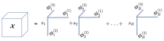
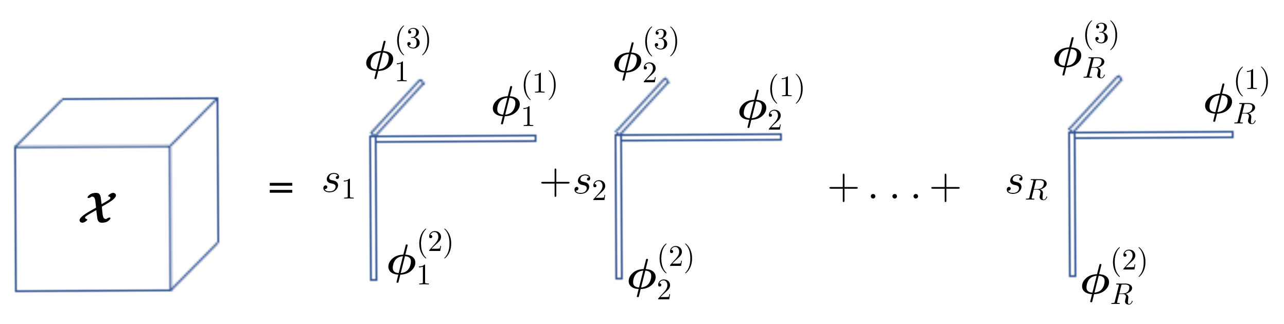
The rank-R CPD of order Q is defined according to

$$\begin{array}{c}\hfill \mathcal{X}=\sum _{r=1}^R{s}_r\underset{{\mathcal{X}}_r}{\underbrace{\left({\mathit{\varphi }}_r^{\left(1\right)}\circ \dots \circ {\mathit{\varphi }}_r^{\left(Q\right)}\right)}}with\mathrm{rank}\left\{{\mathcal{X}}_r\right\}=1\end{array}$$

where ○ is the outer product [25], ${\mathit{\varphi }}_r^{\left(q\right)}\in {\mathbb{R}}^{N_q\times 1}$ and $s_r$ is a real scalar.

An equivalent formulation using the q-mode product defined in Definition 3 is

$$\mathcal{X}=\mathcal{S}{\times }_1{\mathbf{\Phi }}^{\left(1\right)}{\times }_2\dots {\times }_Q{\mathbf{\Phi }}^{\left(Q\right)}$$

where $\mathcal{S}$ is the $R\times \dots \times R$ diagonal core tensor with ${\left[\mathcal{S}\right]}_{r,\dots ,r}=s_r$ and ${\mathbf{\Phi }}^{\left(q\right)}=[{\mathit{\varphi }}_1^{\left(q\right)}\dots {\mathit{\varphi }}_R^{\left(q\right)}]$ is the q-th factor matrix of size $N_q\times R$.

The q-mode unfolding matrix for tensor $\mathcal{X}$ is given by

$${\mathit{X}}_{\left(q\right)}={\mathbf{\Phi }}^{\left(q\right)}\mathit{S}{\left({\mathbf{\Phi }}^{\left(Q\right)}\odot \dots \odot {\mathbf{\Phi }}^{(q+1)}\odot {\mathbf{\Phi }}^{(q-1)}\odot \dots \odot {\mathbf{\Phi }}^{\left(1\right)}\right)}^T$$

where $\mathit{S}=\mathrm{diag}\left(\mathit{s}\right)$ with $\mathit{s}={[s_1,\dots ,s_R]}^T$ and ⊙ stands for the Khatri-Rao product [25].

2.1.3. Tucker Decomposition (TKD)

The Tucker tensor model of order Q is defined according to

$$\begin{array}{c}\hfill \mathcal{X}=\sum _{m_1=1}^{M_1}\sum _{m_2=1}^{M_2}\cdots \sum _{m_Q=1}^{M_Q}{s}_{m_1{m}_2\dots m_Q}\left({\mathit{\varphi }}_{m_1}^{\left(1\right)}\circ {\mathit{\varphi }}_{m_2}^{\left(2\right)}\circ \cdots \circ {\mathit{\varphi }}_{m_Q}^{\left(Q\right)}\right)\end{array}$$

where ${\mathit{\varphi }}_{m_q}^{\left(q\right)}\in {\mathbb{R}}^{N_q\times 1}$, $q=1,\dots ,Q$ and $s_{m_1{m}_2\dots m_Q}$ is a real scalar.

The q-mode product of $\mathcal{X}$ is similar to CPD case, however the q-mode unfolding matrix for tensor $\mathcal{X}$ is slightly different

$$\begin{array}{c}\hfill {\mathbf{X}}_{\left(q\right)}={\mathbf{\Phi }}^{\left(q\right)}{\mathbf{S}}_{\left(q\right)}{\left({\mathbf{\Phi }}^{\left(Q\right)}\otimes \dots \otimes {\mathbf{\Phi }}^{(q+1)}\otimes {\mathbf{\Phi }}^{(q-1)}\dots \otimes {\mathbf{\Phi }}^{\left(1\right)}\right)}^T\end{array}$$

where ${\mathbf{S}}_{\left(q\right)}\in {\mathbb{R}}^{N_q\times N_1{N}_2\dots N_{q-1}{N}_{q+1}\dots N_Q}$ the q-mode unfolding matrix of tensor $\mathcal{S}$, ${\mathbf{\Phi }}^{\left(q\right)}=[{\mathit{\varphi }}_1^{\left(q\right)}\dots {\mathit{\varphi }}_{M_q}^{\left(q\right)}]\in {\mathbb{R}}^{N_q\times M_q}$ and ⊗ stands for Kronecker product. See Figure 1.

Figure 1. Canonical Polyadic Decomposition (CPD).

Following the definitions, we note that the CPD and TKD scenarios imply that vector $\mathbf{x}$ in Equation (11) is related either to the structured linear system ${\mathbf{\Phi }}^{\odot }={\mathbf{\Phi }}^{\left(Q\right)}\odot \dots \odot {\mathbf{\Phi }}^{(q+1)}\odot {\mathbf{\Phi }}^{(q-1)}\odot \dots \odot {\mathbf{\Phi }}^{\left(1\right)}$ or ${\mathbf{\Phi }}^{\otimes }={\mathbf{\Phi }}^{\left(Q\right)}\otimes \dots \otimes {\mathbf{\Phi }}^{(q+1)}\otimes {\mathbf{\Phi }}^{(q-1)}\dots \otimes {\mathbf{\Phi }}^{\left(1\right)}$.

2.2. The Marchenko-Pastur Distribution

The Marchenko-Pastur distribution was introduced half a century ago [45] in 1967, and plays a key role in a number of high-dimensional signal processing problems. To help the reader, in this section, we introduce some fundamental results concerning large empirical covariance matrices. Let ${\left({\mathbf{v}}_n\right)}_{n=1,\dots ,N}$ a sequence of i.i.d zero mean Gaussian random M-dimensional vectors for which $\mathbb{E}\left({\mathit{v}}_n{\mathit{v}}_n^T\right)={\sigma }^2{\mathit{I}}_M$. We consider the empirical covariance matrix

$$\frac{1}{N}\sum _{n=1}^N{\mathit{v}}_n{\mathit{v}}_n^T$$

which can be also written as

$$\frac{1}{N}\sum _{n=1}^N{\mathit{v}}_n{\mathit{v}}_n^T={\mathit{W}}_N{\mathit{W}}_N^T$$

where matrix ${\mathit{W}}_N$ is defined by ${\mathit{W}}_N=\frac{1}{\sqrt{N}}[{\mathit{v}}_1,\dots ,{\mathit{v}}_N]$. ${\mathit{W}}_N$ is thus a Gaussian matrix with independent identically distributed $\mathcal{N}(0,\frac{{\sigma }^2}{N})$ entries. When $N\to +\infty$ while M remains fixed, matrix ${\mathit{W}}_N{\mathit{W}}_N^T$ converges towards ${\sigma }^2{\mathit{I}}_M$ in the spectral norm sense. In the high dimensional asymptotic regime defined by

$$M\to +\infty ,N\to +\infty ,c_N=\frac{M}{N}\to c>0$$

it is well understood that $∥{\mathit{W}}_N{\mathit{W}}_N^T-{\sigma }^2{\mathit{I}}_M∥$ does not converge towards 0. In particular, the empirical distribution ${\widehat{\nu }}_N=\frac{1}{M}{\sum }_{m=1}^M{\delta }_{{\widehat{\lambda }}_{m,N}}$ of the eigenvalues ${\widehat{\lambda }}_{1,N}\ge \dots \ge {\widehat{\lambda }}_{M,N}$ of ${\mathit{W}}_N{\mathit{W}}_N^T$ does not converge towards the Dirac measure at point $\lambda ={\sigma }^2$. More precisely, we denote by ${\nu }_{c,{\sigma }^2}$ the Marchenko-Pastur distribution of parameters $(c,{\sigma }^2)$ defined as the probability measure

$$\begin{array}{c}\hfill {\nu }_{c,{\sigma }^2}\left(d\lambda \right)={\delta }_0{[1-\frac{1}{c}]}_{+}+\frac{\sqrt{(\lambda -{\lambda }^{-})({\lambda }^{+}-\lambda )}}{2{\sigma }^{2}c\pi \lambda }{⊮}_{[{\lambda }^{-},{\lambda }^{+}]\left(\lambda \right)}d\lambda \end{array}$$

(1)

with ${\lambda }^{-}={\sigma }^2{(1-\sqrt{c})}^2$ and ${\lambda }^{+}={\sigma }^2{(1+\sqrt{c})}^2$. Then, the following result holds.

Theorem 1 

([45]). The empirical eigenvalue value distribution ${\widehat{\nu }}_N$ converges weakly almost surely towards ${\nu }_{c,{\sigma }^2}$ when both M and N converge towards $+\infty$ in such a way that $c_N=\frac{M}{N}$ converges towards $c>0$. Moreover, it holds that

$$\begin{array}{cc}\hfill {\widehat{\lambda }}_{1,N}& \to {\sigma }^2{(1+\sqrt{c})}^{2}a.s.\end{array}$$

(2)

$$\begin{array}{cc}\hfill {\widehat{\lambda }}_{min(M,N)}& \to {\sigma }^2{(1-\sqrt{c})}^{2}a.s.\end{array}$$

(3)

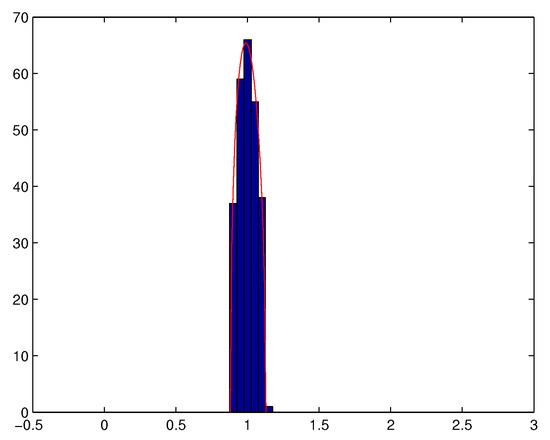
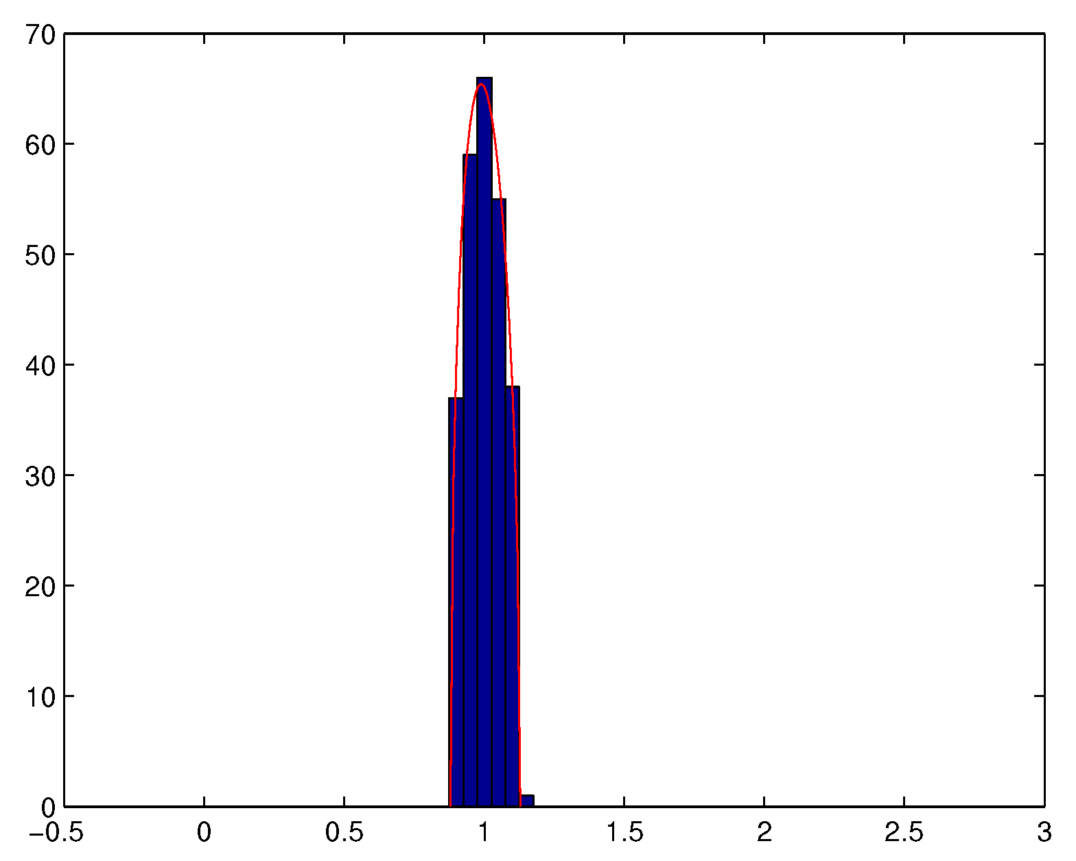
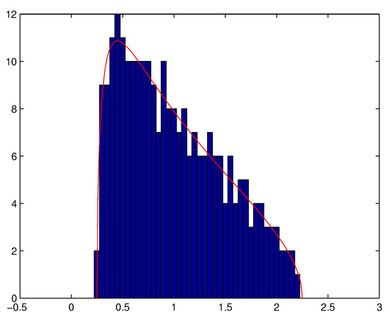
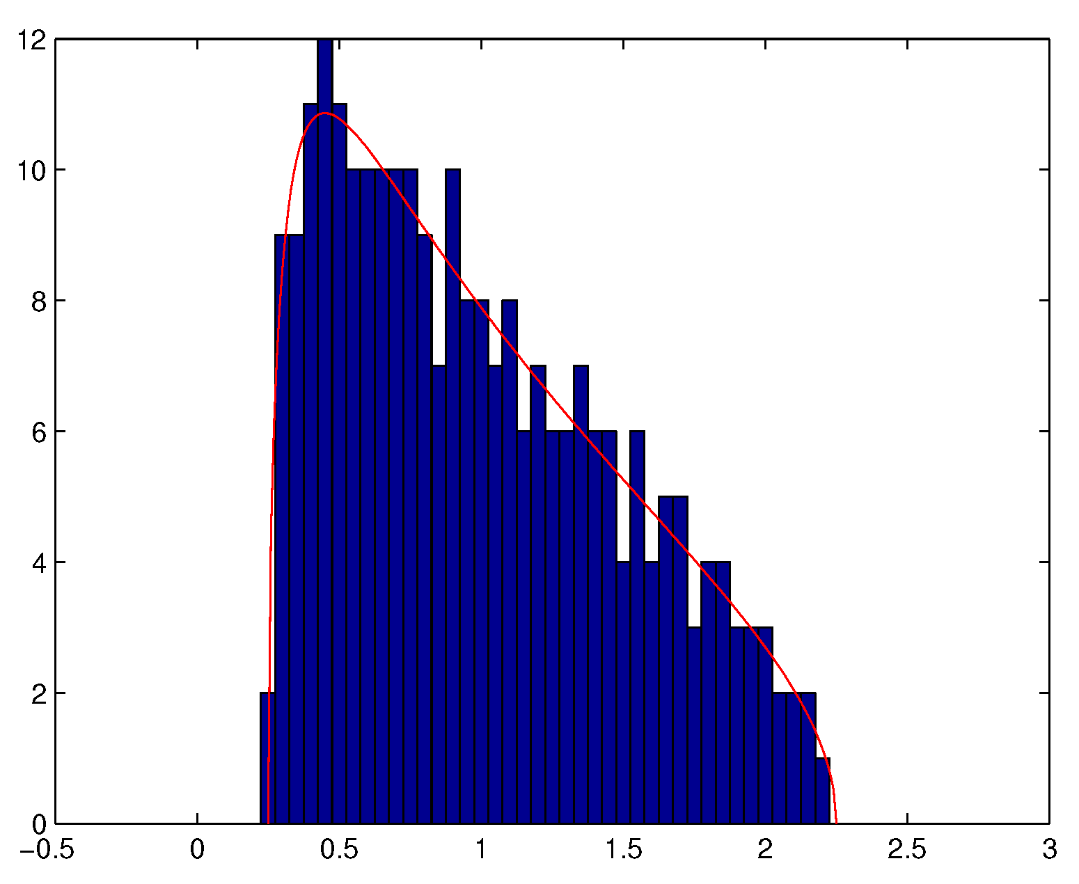
We also observe that Theorem 1 remains valid if ${\mathbf{W}}_N$ is not necessarily a Gaussian matrix whose i.i.d. elements have a finite fourth order moment (see e.g., [43]). Theorem 1 means that when ratio $\frac{M}{N}$ is not small enough, the eigenvalues of the empirical spatial covariance matrix of a temporally and spatially white noise tend to spread out around the variance of the noise, and that almost surely, for N large enough, all the eigenvalues are located in a neighbourhood of interval $[{\lambda }^{-},{\lambda }^{+}]$. See Figure 2 and Figure 3.

Figure 2. Histogram of the eigenvalues of $\frac{{\mathbf{W}}_N{\mathbf{W}}_N^T}{N}$ (with $M=256,c_N=\frac{M}{N}=\frac{1}{256}$, ${\sigma }^2=1$).

Figure 3. Histogram of the eigenvalues of $\frac{{\mathbf{W}}_N{\mathbf{W}}_N^T}{N}$ (with $M=256,c_N=\frac{M}{N}=\frac{1}{4}$, ${\sigma }^2=1$).

3. Classification in a Computational Information Geometry (CIG) Framework

3.1. Formulation Based on a $\mathrm{SNR}$-Type Criterion

We denote by $\mathrm{SNR}={\sigma }_{\mathbf{s}}^2/{\sigma }^2$ and $p_i(·)=p(·|{\mathcal{H}}_i)$ with $i\in \{0,1\}$. The binary classification of the random signal based on the equi-probable binary hypothesis test, $\mathbf{s}$, is

$$\begin{array}{c}\hfill \left\{\begin{array}{c}{\mathcal{H}}_0:p_0({\mathbf{y}}_N;\mathbf{\Phi },\mathrm{SNR}=0)=\mathcal{N}\left(\mathbf{0},{\mathbf{\Sigma }}_0\right),\hfill \\ {\mathcal{H}}_1:p_1({\mathbf{y}}_N;\mathbf{\Phi },\mathrm{SNR}\ne 0)=\mathcal{N}\left(\mathbf{0},{\mathbf{\Sigma }}_1\right)\hfill \end{array}\right.\end{array}$$

(4)

where ${\mathbf{\Sigma }}_0={\sigma }^2{\mathbf{I}}_N$ and ${\mathbf{\Sigma }}_1={\sigma }^2\left(\mathrm{SNR}\times \mathbf{\Phi }{\mathbf{\Phi }}^T+{\mathbf{I}}_N\right)$. The null hypothesis data-space (${\mathcal{H}}_0$) is defined as ${\mathcal{X}}_0=\mathcal{X}\backslash {\mathcal{X}}_1$ where

$$\begin{array}{c}\hfill {\mathcal{X}}_1=\left\{{\mathbf{y}}_N:\mathsf{\Lambda }\left({\mathbf{y}}_N\right)=log\frac{p_1\left({\mathbf{y}}_N\right)}{p_0\left({\mathbf{y}}_N\right)}>{\tau }^{\prime }\right\}\end{array}$$

is the alternative hypothesis (${\mathcal{H}}_1$) data-space. Following the above expression, the log-likelihood ratio test $\mathsf{\Lambda }\left({\mathbf{y}}_N\right)$ and the binary classification threshold ${\tau }^{\prime }$ are given by

$$\begin{array}{cc}\hfill \mathsf{\Lambda }\left({\mathbf{y}}_N\right)& =\frac{{\mathbf{y}}_N^T\mathbf{\Phi }{\left({\mathbf{\Phi }}^T\mathbf{\Phi }+\mathrm{SNR}\times \mathbf{I}\right)}^{-1}{\mathbf{\Phi }}^T{\mathbf{y}}_N}{{\sigma }^2},\hfill \\ \hfill {\tau }^{\prime }& =-log\det \left(\mathrm{SNR}\times \mathbf{\Phi }{\mathbf{\Phi }}^T+{\mathbf{I}}_N\right)\hfill \end{array}$$

where $\det (·)$ and $log(·)$ are respectively the determinant and the natural logarithm.

3.2. The Expected Log-likelihood Ratio in Geometry Perspective

We note that the estimated hypothesis $\widehat{\mathcal{H}}$ is associated to $p({\mathbf{y}}_N|\widehat{\mathcal{H}})=\mathcal{N}\left(\mathbf{0},\mathbf{\Sigma }\right)$. Therefore, the expected log-likelihood ratio is defined by

$$\begin{array}{cc}\hfill {\mathbb{E}}_{{\mathbf{y}}_N|\widehat{\mathcal{H}}}\mathsf{\Lambda }\left({\mathbf{y}}_N\right)& ={\int }_{\mathcal{X}}p({\mathbf{y}}_N|\widehat{\mathcal{H}})log\frac{p_1\left({\mathbf{y}}_N\right)}{p_0\left({\mathbf{y}}_N\right)}d{\mathbf{y}}_N\hfill \\ & =\mathcal{KL}(\widehat{\mathcal{H}}\left|\right|{\mathcal{H}}_0)-\mathcal{KL}(\widehat{\mathcal{H}}\left|\right|{\mathcal{H}}_1)\hfill \\ & =\frac{1}{{\sigma }^2}\mathrm{Tr}\left\{{\left({\mathbf{\Phi }}^T\mathbf{\Phi }+\mathrm{SNR}\times \mathbf{I}\right)}^{-1}{\mathbf{\Phi }}^T\mathbf{\Sigma }\mathbf{\Phi }\right\}\hfill \end{array}$$

where

$$\begin{array}{c}\hfill \mathcal{KL}(\widehat{\mathcal{H}}\left|\right|{\mathcal{H}}_i)={\int }_{\mathcal{X}}p({\mathbf{y}}_N|\widehat{\mathcal{H}})log\frac{p({\mathbf{y}}_N|\widehat{\mathcal{H}})}{p_i\left({\mathbf{y}}_N\right)}d{\mathbf{y}}_N\end{array}$$

is the Kullback-Leibler Divergence (KLD) [10]. The expected log-likelihood ratio test admits to a simple geometric characterization based on the difference of two KLDs [8]. However, it is often difficult to evaluate the performance of the test via the minimal Bayes’ error probability $P_e^{\left(N\right)}$, since its expression cannot be determined analytically in closed-form [3,8].

The minimal Bayes’ error probability conditionally to vector ${\mathbf{y}}_N$ is defined as

$$\begin{array}{c}\hfill \mathrm{Pr}\left(\mathrm{Error}\right|{\mathbf{y}}_N)=\frac{1}{2}min\{P_{1,0},P_{0,1}\}\end{array}$$

where $P_{i,i^{\prime }}=\mathrm{Pr}\left({\mathcal{H}}_i\right|{\mathbf{y}}_N\in {\mathcal{X}}_{i^{\prime }})$.

3.3. CUB

According to [24], the relation between the Chernoff Upper Bound and the (average) minimal Bayes’ error probability $P_e^{\left(N\right)}=\mathbb{E}\mathrm{Pr}\left(\mathrm{Error}\right|{\mathbf{y}}_N)$ is given by

$$\begin{array}{c}\hfill P_e^{\left(N\right)}\le \frac{1}{2}\times exp[-{\tilde{\mu }}_N\left(s\right)]\end{array}$$

(5)

where the (Chernoff) s-divergence for $s\in (0,1)$ is given by

$$\begin{array}{c}\hfill {\tilde{\mu }}_N\left(s\right)=-log{M}_{\mathsf{\Lambda }\left({\mathbf{y}}_N\right|{\mathcal{H}}_1)}(-s)\end{array}$$

(6)

in which $M_X\left(t\right)=\mathbb{E}exp[t\times X]$ is the moment generating function (mgf) of variable X. The error exponent, denoted by $\tilde{\mu }\left(s\right)$, is given by the Chernoff information which is an asymptotic characterization on the exponentially decay of the minimal Bayes’ error probability. The error exponent is derived thanks to the Stein’s lemma according to [13]

$$\begin{array}{c}\hfill -\underset{N\to \infty }{lim}\frac{log{P}_e^{\left(N\right)}}{N}=\underset{N\to \infty }{lim}\frac{{\tilde{\mu }}_N\left(s\right)}{N}\stackrel{\mathrm{def}.}{=}\tilde{\mu }\left(s\right).\end{array}$$

As parameter $s\in (0,1)$ is free, the CUB can be tightened by minimizing this parameter:

$$\begin{array}{c}\hfill s^{\star }=arg\underset{s\in (0,1)}{max}\tilde{\mu }\left(s\right).\end{array}$$

(7)

Finally, using Equations (5) and (7), the Chernoff Upper Bound (CUB) is obtained. Instead of solving Equation (7), the Bhattacharyya Upper Bound (BUB) is calculated by Equation (5) and by fixing $s=1/2$ . Therefore we have the following relation of order:

$$\begin{array}{c}\hfill P_e^{\left(N\right)}\le \frac{1}{2}\times exp[-{\tilde{\mu }}_N\left(s^{\star }\right)]\le \frac{1}{2}\times exp[-{\tilde{\mu }}_N(1/2)].\end{array}$$

Lemma 1.

The log-moment generating function given by Equation (6) for test of Equation (4) is given by

$$\begin{array}{cc}\hfill {\tilde{\mu }}_N\left(s\right)& =-\frac{1-s}{2}logdet\left(\mathrm{SNR}\times \mathbf{\Phi }{\mathbf{\Phi }}^T+\mathbf{I}\right)\hfill \\ & +\frac{1}{2}logdet\left(\mathrm{SNR}\times (1-s)\mathbf{\Phi }{\mathbf{\Phi }}^T+\mathbf{I}\right).\hfill \end{array}$$

(8)

Proof. 

See Appendix A. ◻

From now on, to simplify the presentation and the numerical results later on, we denote by

$$\begin{array}{c}\hfill {\mu }_N\left(s\right)=-{\tilde{\mu }}_N\left(s\right)\\ \hfill \mu \left(s\right)=-\tilde{\mu }\left(s\right)\end{array}$$

for all $s\in [0,1]$, the opposites of the log-moment generating function and its limit.

Remark 1.

The functions ${\mu }_N\left(s\right),\mu \left(s\right)$ are negative, since the s-divergence ${\tilde{\mu }}_N\left(s\right)$ is positive for all $s\in [0,1]$.

3.4. Fisher Information

In the small deviation regime, we assume that $\delta \mathrm{SNR}$ is a small deviation of the SNR. The new binary hypothesis test is

$$\begin{array}{c}\hfill \left\{\begin{array}{ccc}{\mathcal{H}}_0& :& \mathbf{y}|\delta \mathrm{SNR}=0\sim \mathcal{N}\left(\mathbf{0},\mathbf{\Sigma }\left(0\right)\right),\hfill \\ {\mathcal{H}}_1& :& \mathbf{y}|\delta \mathrm{SNR}\ne 0\sim \mathcal{N}\left(\mathbf{0},\mathbf{\Sigma }\left(\delta \mathrm{SNR}\right)\right)\hfill \end{array}\right.\end{array}$$

where $\mathbf{\Sigma }\left(x\right)=x\times \mathbf{\Phi }{\mathbf{\Phi }}^T+\mathbf{I}.$ The s-divergence in the small $\mathrm{SNR}$ deviation scenario is written as

$${\mu }_N\left(s\right)=\frac{1-s}{2}logdet\left[\mathbf{\Sigma }\left(\delta \mathrm{SNR}\right)\right]-\frac{1}{2}logdet\left[\mathbf{\Sigma }(\delta \mathrm{SNR}\times (1-s\left)\right)\right]$$

Lemma 2.

The s-divergence in the small deviation regime can be approximated according to

$$\begin{array}{c}\hfill \frac{{\mu }_N\left(s\right)}{N}\stackrel{\delta \mathrm{SNR}\ll 1}{\approx }(s-1)s\times \frac{{\left(\delta \mathrm{SNR}\right)}^2}{2}\times \frac{{\mathrm{J}}_F\left(0\right)}{N}\end{array}$$

where the Fisher information [3] is given by

$$\begin{array}{c}\hfill {\mathrm{J}}_F\left(x\right)=\frac{1}{2}\mathrm{Tr}({(\mathbf{I}+x\times \mathbf{\Phi }{\mathbf{\Phi }}^T)}^{-1}\mathbf{\Phi }{\mathbf{\Phi }}^T{(\mathbf{I}+x\times \mathbf{\Phi }{\mathbf{\Phi }}^T)}^{-1}\mathbf{\Phi }{\mathbf{\Phi }}^T).\end{array}$$

Proof. 

See Appendix B. ◻

According to Lemma 2, the optimal s-value at low $\mathrm{SNR}$ is $s^{\star }\stackrel{\delta \mathrm{SNR}\ll 1}{=}\frac{1}{2}$. At contrary, the optimal s-value for larger $\mathrm{SNR}$ is given by the following lemma.

Lemma 3.

In case of large $\mathrm{SNR}$, we have

$$\begin{array}{c}\hfill s^{\star }\stackrel{\mathrm{SNR}\gg 1}{\approx }1-\frac{1}{log\mathrm{SNR}+\frac{1}{K}{\sum }_{n=1}^{K}log{\lambda }_n}.\end{array}$$

(9)

where ${\left({\lambda }_n\right)}_{n=1,\dots ,N}$ are the eigenvalues of $\mathbf{\Phi }{\mathbf{\Phi }}^T$.

Proof. 

See Appendix C. ◻

4. Computational Information Geometry for Classification

4.1. Formulation of the Observation Vector as a Structured Linear Model

The measurement tensor follows a noisy Q-order tensor of size $N_1\times \dots \times N_Q$ can be expressed as

$$\begin{array}{c}\hfill \mathcal{Y}=\mathcal{X}+\mathcal{N}\end{array}$$

(10)

where $\mathcal{N}$ is the noise tensor whose entries are assumed to be centered i.i.d. Gaussian, i.e., ${\left[\mathcal{N}\right]}_{n_1,\dots ,n_Q}\sim \mathcal{N}(0,{\sigma }^2)$ and the core tensor $\mathcal{X}$ follows either CPD or TKD given by Section 2.1.2 and Section 2.1.3, respectively. The vectorization of Equation (10) is given by

$$\begin{array}{c}\hfill {\mathbf{y}}_N=\mathrm{vec}\left({\mathbf{Y}}_{\left(1\right)}\right)=\mathbf{x}+\mathbf{n}\end{array}$$

(11)

where $\mathbf{n}=\mathrm{vec}\left({\mathbf{N}}_{\left(1\right)}\right)$ and $\mathbf{x}=\mathrm{vec}\left({\mathbf{X}}_{\left(1\right)}\right)$. Note that ${\mathbf{Y}}_{\left(1\right)}$, ${\mathbf{N}}_{\left(1\right)}$ and ${\mathbf{X}}_{\left(1\right)}$ are respectively the first unfolding matrices given by Definition 4 of tensors $\mathcal{Y},\mathcal{N}$ and $\mathcal{X}$,

• When tensor $\mathcal{X}$ follows a Q-order CPD with a canonical rank of M, we have

  $$\begin{array}{c}\hfill \mathbf{x}=\mathrm{vec}\left\{{\mathbf{\Phi }}^{\left(1\right)}\mathbf{S}{\left({\mathbf{\Phi }}^{\left(Q\right)}\odot \dots \odot {\mathbf{\Phi }}^{\left(2\right)}\right)}^T\right\}={\mathbf{\Phi }}^{\odot }{s}\end{array}$$

  where ${\mathbf{\Phi }}^{\odot }={\mathbf{\Phi }}^{\left(Q\right)}\odot \dots \odot {\mathbf{\Phi }}^{\left(1\right)}$ is a $N\times R$ structured matrix and ${s}={\left[\begin{array}{ccc}{s}_1& \dots & s_R\end{array}\right]}^T$ where $s_r\sim \mathcal{N}(0,{\sigma }_s^2)$, i.i.d. and $N=N_1\dots N_Q$.
• When tensor $\mathcal{X}$ follows a Q-order TKD of multilinear rank of $\{M_1,\dots ,M_Q\}$, we have

  $$\begin{array}{c}\hfill \mathbf{x}=\mathrm{vec}\left\{{\mathbf{\Phi }}^{\left(1\right)}{\mathbf{S}}_{\left(1\right)}{\left({\mathbf{\Phi }}^{\left(Q\right)}\otimes \dots \otimes {\mathbf{\Phi }}^{\left(2\right)}\right)}^T\right\}={\mathbf{\Phi }}^{\otimes }\mathrm{vec}\left(\mathcal{S}\right)\end{array}$$

  where ${\mathbf{\Phi }}^{\otimes }={\mathbf{\Phi }}^{\left(Q\right)}\otimes \dots \otimes {\mathbf{\Phi }}^{\left(1\right)}$ is a $N\times M$ structured matrix with $M=M_1\dots M_Q$ and $\mathrm{vec}\left(\mathcal{S}\right)$ is the vectorization of tensor $\mathcal{S}$ where $s_{m_1,\dots ,.m_Q}\sim \mathcal{N}(0,{\sigma }_s^2)$, i.i.d.

4.2. The CPD Case

We recall that in the CPD case, matrix ${\mathbf{\Phi }}^{\odot }={\mathbf{\Phi }}^{\left(Q\right)}\odot \dots \odot {\mathbf{\Phi }}^{\left(1\right)}$ and ${\left({\mathbf{\Phi }}^{\left(q\right)}\right)}_{q=1,\dots ,Q}$ are matrices of size $N_q\times R$. In the following, we assume that matrices ${\mathbf{\Phi }}_{q=1,\dots ,Q}^{\left(q\right)}$ are random matrices with Gaussian $\mathcal{N}(0,\frac{1}{N_q})$ variate entries. We evaluate the behavior of $\frac{{\mu }_N\left(s\right)}{N}$ when ${\left(N_q\right)}_{q=1,\dots ,Q}$ converge towards $+\infty$ at the same rate and that $\frac{R}{N}$ converges towards a non zero limit.

Result 1.

In the asymptotic regime where $N_1,\dots ,N_Q$ converge towards $+\infty$ at the same rate and where $R\to +\infty$ in such a way that $c_R=\frac{R}{N}$ converges towards a finite constant $c>0$, it holds that

$$\begin{array}{cc}\hfill \frac{{\mu }_N\left(s\right)}{N}& \stackrel{\mathrm{a}.\mathrm{s}}{⟶}\mu \left(s\right)=\frac{1-s}{2}{\mathbf{\Psi }}_c\left(\mathrm{SNR}\right)-\frac{1}{2}{\mathbf{\Psi }}_c((1-s)\times \mathrm{SNR})\hfill \end{array}$$

(12)

with $\mathrm{a}.\mathrm{s}$ standing for “almost sure convergence” and

$$\begin{array}{cc}\hfill {\mathbf{\Psi }}_c\left(x\right)& =log\left(1+\frac{2c}{u\left(x\right)+(1-c)}\right)\hfill \\ & +c\times log\left(1+\frac{2}{u\left(x\right)-(1-c)}\right)\hfill \\ & -\frac{4c}{x(u{\left(x\right)}^2-{(1-c)}^2)}\hfill \end{array}$$

(13)

with $u\left(x\right)=\frac{1}{x}+\sqrt{(\frac{1}{x}+{\lambda }_c^{+})(\frac{1}{x}+{\lambda }_c^{-})}$ where ${\lambda }_c^{\pm }={(1\pm \sqrt{c})}^2$.

Proof. 

See Appendix D. ◻

Remark 2.

In [49], the Central Limit Theorem (CLT) for the linear eigenvalue statistics of the tensor version of the sample covariance matrix of type ${\mathbf{\Phi }}^{\odot }{\left({\mathbf{\Phi }}^{\odot }\right)}^T$ is established, for ${\mathbf{\Phi }}^{\odot }={\mathbf{\Phi }}^{\left(2\right)}\odot {\mathbf{\Phi }}^{\left(1\right)}$, i.e., the tensor order is $Q=2$.

4.2.1. Small $\mathrm{SNR}$ Deviation Scenario

In this section, we assume that $\mathrm{SNR}$ is small. Under this regime, we have the following result:

Result 2.

In the small $\mathrm{SNR}$ scenario, the Fisher information for CPD is given as

$$\begin{array}{c}\hfill \mu \left(\frac{1}{2}\right)\stackrel{\mathrm{SNR}\ll 1}{\approx }-\frac{{\left(\mathrm{SNR}\right)}^2}{16}\times c(1+c).\end{array}$$

Proof. 

Using Lemma 2, we can notice that

$$\frac{{\mathrm{J}}_F\left(0\right)}{N}=\frac{1}{2}\frac{R}{N}\frac{1}{R}\mathrm{Tr}\left[{({\mathbf{\Phi }}^{\odot }{\left({\mathbf{\Phi }}^{\odot }\right)}^T)}^2\right]$$

and that

$$\frac{1}{R}\mathrm{Tr}\left[{({\mathbf{\Phi }}^{\odot }{\left({\mathbf{\Phi }}^{\odot }\right)}^T)}^2\right]$$

converges a.s towards the second moment of the Marchenko-Pastur distribution which is $1+c$ (see for instance [43]). ◻

Note that $\mu \left(\frac{1}{2}\right)$ is the error exponent related to the Bhattacharyya divergence.

4.2.2. Large $\mathrm{SNR}$ Deviation Scenario

Result 3.

In case of large $\mathrm{SNR}$, the minimizer of Chernoff Information is given by

$$\begin{array}{c}\hfill s^{\star }\stackrel{\mathrm{SNR}\gg 1}{\approx }1-\frac{1}{log\mathrm{SNR}-1-\frac{1-c}{c}log(1-c)}.\end{array}$$

(14)

Proof. 

It is straightforward to notice that

$$\frac{1}{K}\sum _{n=1}^{K}log\left({\lambda }_n\right)⟶{\int }_0^{+\infty }log\left(\lambda \right)d{\nu }_c\left(\lambda \right)=-1-\frac{1-c}{c}log(1-c).$$

The last equality can be obtained as in [50]. Using Lemma 3, we get immediately Equation (14). ◻

Remark 3.

It is interesting to note that for $c\to 0$ or 1, the optimal s-value follows the same approximated relation given by

$$\begin{array}{c}\hfill s^{\star }\stackrel{\mathrm{SNR}\gg 1}{\approx }1-\frac{1}{log\mathrm{SNR}}\end{array}$$

as long as $\mathrm{SNR}\gg exp\left[1\right]$ or equivalently a $\mathrm{SNR}$ in dB much larger than 4 dB.

Proof. 

It is straightforward to note that

$$\begin{array}{c}\hfill \frac{1-c}{c}log(1-c)\stackrel{c\to 1}{⟶}0,and\frac{1-c}{c}log(1-c)\stackrel{c\to 0}{⟶}-1.\end{array}$$

Using Equation (14) and condition $\mathrm{SNR}\gg exp\left[1\right]$, the desired result is proved. ◻

4.2.3. Approximated Analytical Expressions for $c\ll 1$ and Any $\mathrm{SNR}$

In the case of low rank CPD where its rank R is supposed to be small compared to N, it is realistic to assume $c\ll 1$ since $R\ll N$.

Result 4.

Under this regime, the error exponent can be approximated as follows:

$$\begin{array}{c}\hfill \mu \left(s\right)\stackrel{c\ll 1}{\approx }\frac{c}{2}\left((1-s)log(1+\mathrm{SNR})-log(1+(1-s\left)\mathrm{SNR}\right)\right).\end{array}$$

Proof. 

See Appendix E. ◻

It is easy to notice that the second-order derivative of $\mu \left(s\right)$ is strictly positive. Therefore, $\mu \left(s\right)$ is a strictly convex function over interval $(0,1)$. As a consequence, $\mu \left(s\right)$ admits at most one global minimum. We denote by $s^{\star }$, the global minimizer and obtained by zeroing the first-order derivative of the error exponent. This optimal value is expressed as

$$\begin{array}{c}\hfill s^{\star }\stackrel{c\ll 1}{\approx }1+\frac{1}{\mathrm{SNR}}-\frac{1}{log(1+\mathrm{SNR})}.\end{array}$$

(15)

The two following scenarios can be considered:

• At low $\mathrm{SNR}$, we denote by $\mu \left(s^{\star }\right)$, the error exponent associated with the tightest CUB, coincides with the error exponent associated with the BUB. To see this, when $c\ll 1$, we derive the second-order approximation of the optimal value $s^{\star }$ in Equation (47)

  $$\begin{array}{cc}\hfill s^{\star }& \stackrel{2}{\approx }1+\frac{1}{\mathrm{SNR}}\left(1-\left(1+\frac{\mathrm{SNR}}{2}\right)\right)=\frac{1}{2}.\hfill \end{array}$$
  Result 1 and the above approximation allow us to get the best error exponent at low $\mathrm{SNR}$ and $c\ll 1$,

  $$\begin{array}{cc}\hfill \mu \left(\frac{1}{2}\right)& \stackrel{\mathrm{SNR}\ll 1}{\approx }\frac{1}{4}{\mathbf{\Psi }}_{c\ll 1}\left(\mathrm{SNR}\right)-\frac{1}{2}{\mathbf{\Psi }}_{c\ll 1}\left(\frac{\mathrm{SNR}}{2}\right)\hfill \\ & =\frac{c}{2}log\frac{\sqrt{1+\mathrm{SNR}}}{1+\frac{\mathrm{SNR}}{2}}.\hfill \end{array}$$
• Contrarily, when $\mathrm{SNR}\to \infty$, $s^{\star }\to 1$. As a consequence, the optimal error exponent in this regime is not the BUB anymore. Assuming that $\frac{log\mathrm{SNR}}{\mathrm{SNR}}\to 0$, Equation (15) in Result 4 provides the following approximation of the optimal error exponent for large $\mathrm{SNR}$

  $$\begin{array}{c}\hfill \mu \left(s^{\star }\right)\stackrel{\mathrm{SNR}\gg 1}{\approx }\frac{c}{2}\left(1-log\mathrm{SNR}+loglog(1+\mathrm{SNR})\right).\end{array}$$

4.3. The TKD Case

In the TKD case, we recall that matrix ${\mathbf{\Phi }}^{\otimes }={\mathbf{\Phi }}^{\left(Q\right)}\otimes \dots \otimes {\mathbf{\Phi }}^{\left(1\right)}$, with ${\left({\mathit{\varphi }}^{\left(q\right)}\right)}_{1\le q\le Q}$ are $N_q\times M_q$ dimensional matrices. We still assume that matrices ${\mathbf{\Phi }}_{q=1,\dots ,Q}^{\left(q\right)}$ are random matrices with Gaussian $\mathcal{N}(0,\frac{1}{N_q})$ entries.

Result 5.

In the asymptotic regime where $M_q<N_q,1\le q\le Q$ and $M_q,N_q$ converge towards $+\infty$ at the same rate such that $\frac{M_q}{N_q}\to c_q$, where $0<c_q<1$, it holds

$$\begin{array}{c}\hfill \frac{{\mu }_N\left(s\right)}{N}\stackrel{\mathrm{a}.\mathrm{s}}{⟶}\mu \left(s\right)=c_1\dots c_Q\left[\frac{1-s}{2}{\int }_0^{+\infty }\dots {\int }_0^{+\infty }log(1+\mathrm{SNR}\times {\lambda }_1\dots {\lambda }_Q)d{\nu }_{c_1}\left({\lambda }_1\right)\dots d{\nu }_{c_Q}\left({\lambda }_Q\right)\right.\\ \hfill \hspace{1em}\hspace{1em}\hspace{1em}\hspace{1em}\hspace{1em}\hspace{1em}-\left.\frac{1}{2}{\int }_0^{+\infty }\dots {\int }_0^{+\infty }log(1+(1-s)\mathrm{SNR}\times {\lambda }_1\dots {\lambda }_Q)d{\nu }_{c_1}\left({\lambda }_1\right)\dots d{\nu }_{c_Q}\left({\lambda }_Q\right)\right]\end{array}$$

where ${\nu }_{c_q}$ are Marchenko-Pastur distributions of parameters $(c_q,1)$ defined as in Equation (1).

Proof. 

See Appendix F. ◻

Remark 4.

We can notice that for $Q=1$, the result 5 is similar to result 1. However, when $Q\ge 2$, the integrals in Equation (16) are not tractable in a closed-form expression. For instance, let $Q=2$, we consider the integral

$$\begin{array}{c}{\int }_{-\infty }^{+\infty }{\int }_{-\infty }^{+\infty }log(1+\mathrm{SNR}\times {\lambda }_1{\lambda }_2){\nu }_{c_1}\left(d{\lambda }_1\right){\nu }_{c_2}\left(d{\lambda }_2\right)\hfill \\ ={\int }_{{\lambda }_{c_1}^{-}}^{{\lambda }_{c_1}^{+}}{\int }_{{\lambda }_{c_2}^{-}}^{{\lambda }_{c_2}^{+}}log(1+\mathrm{SNR}\times {\lambda }_1{\lambda }_2)\frac{\sqrt{\left({\lambda }_1-{\lambda }_{c_1}^{-}\right)\left({\lambda }_{c_1}^{+}-{\lambda }_1\right)}}{2\pi c_1{\lambda }_1}\frac{\sqrt{\left({\lambda }_2-{\lambda }_{c_2}^{-}\right)\left({\lambda }_{c_2}^{+}-{\lambda }_2\right)}}{2\pi c_2{\lambda }_2}d{\lambda }_{1}d{\lambda }_2\hfill \end{array}$$

where ${\lambda }_{c_i}^{\pm }={(1\pm \sqrt{c_i})}^2,i=1,2$. We can notice that this integral is characterized by elliptic integral (see e.g., [51]). As a consequence, it cannot be expressed in closed-form. However, numerical computations can be exploited to solve efficiently the minimization problem of Equation (7).

4.3.1. Large $\mathrm{SNR}$ Deviation Scenario

Result 6.

In case of large $\mathrm{SNR}$, the minimizer of Chernoff Information for TKD is given by

$$\begin{array}{c}\hfill s^{\star }\stackrel{\mathrm{SNR}\gg 1}{\approx }1-\frac{1}{log\mathrm{SNR}-Q-{\sum }_{i=1}^Q\frac{1-c_i}{c_i}log(1-c_i)}.\end{array}$$

Proof. 

We have that

$$\begin{array}{cc}\hfill \frac{1}{M}\sum _{n=1}^{M}log\left({\lambda }_n\right)& ⟶\sum _{q=1}^Q{\int }_0^{+\infty }log\left({\lambda }_q\right)d{\nu }_{c_q}\left({\lambda }_q\right)\hfill \\ & =\sum _{q=1}^Q\left(-1-\frac{1-c_q}{c_q}log(1-c_q)\right)\hfill \\ & =-Q-\sum _{q=1}^Q\frac{1-c_q}{c_q}log(1-c_q).\hfill \end{array}$$

Using Lemma 3, we get immediately Equation (17). ◻

4.3.2. Small $\mathrm{SNR}$ Deviation Scenario

Under this regime, we have the following results

Result 7.

For small $\mathrm{SNR}$ deviation, the Chernoff information for the TKD is given by

$$\begin{array}{c}\hfill \mu \left(\frac{1}{2}\right)\stackrel{\delta \mathrm{SNR}\ll 1}{\approx }-\frac{{\left(\delta \mathrm{SNR}\right)}^2}{16}\prod _{q=1}^Q{c}_q\times (1+c_q).\end{array}$$

Proof. 

Using Lemma 2, we can notice that

$$\frac{{\mathrm{J}}_F\left(0\right)}{N}=\frac{1}{2}\frac{M}{N}\frac{1}{M}\mathrm{Tr}\left[{({\mathbf{\Phi }}^{\otimes }{\left({\mathbf{\Phi }}^{\otimes }\right)}^T)}^2\right]=\frac{1}{2}\frac{M}{N}\prod _{q=1}^Q\frac{\mathrm{Tr}\left[{({\mathbf{\Phi }}^{\left(q\right)}{{\mathbf{\Phi }}^{\left(q\right)}}^T)}^2\right]}{M_q}.$$

Each term in the product converges a.s towards the second moment of Marchenko-Pastur distributions ${\nu }_{c_q}$ which are $1+c_q$ and $\frac{M}{N}$ converges to ${\prod }_{q=1}^Q{c}_q$. This proves the desired result. ◻

Remark 5.

Contrary to the Remark 3, it is interesting to note that for $c_1=c_2=\dots =c_Q=c$ and $c\to 0$ or 1, the optimal s-value follows different approximated relation given by

$$\begin{array}{c}\hfill s^{\star }\underset{c\to 0}{\overset{\mathrm{SNR}\gg 1}{\approx }}1-\frac{1}{log\mathrm{SNR}}\end{array}$$

which does not depend on Q, and

$$\begin{array}{c}\hfill s^{\star }\underset{c\to 1}{\overset{\mathrm{SNR}\gg 1}{\approx }}1-\frac{1}{log\mathrm{SNR}-Q}\end{array}$$

which depends on Q.

In practice, when c is close to 1, we have to carefully check if Q is in the neighbourhood of $log\left(\mathrm{SNR}\right)$. As we can see that, when $log\mathrm{SNR}-Q<0$ or $0<log\mathrm{SNR}-Q<1$, following the above approximation, $s^{\star }\notin [0,1]$.

5. Numerical Illustrations

In this section, we consider cubic tensors of order $Q=3$ with $N_1=10,N_2=20,N_3=30,R=3000$ following a CPD and $M_1=100,M_2=120,M_3=140,N_1=N_2=N_3=200$ for the TKD, respectively.

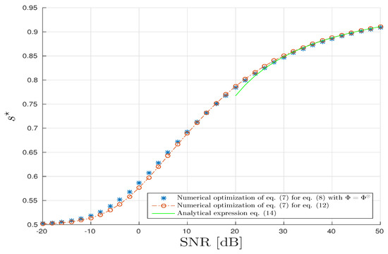
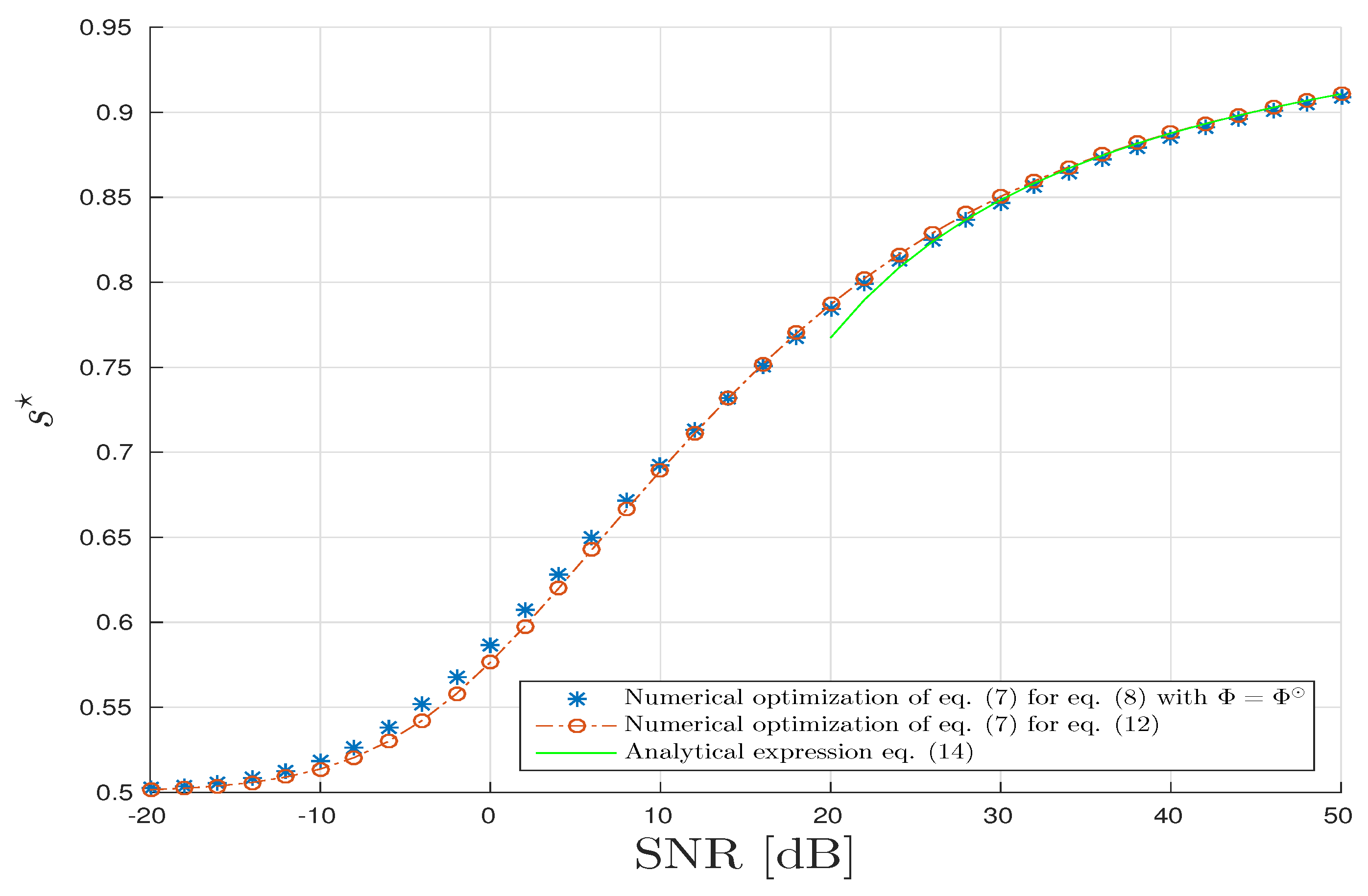
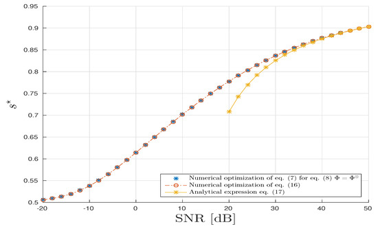
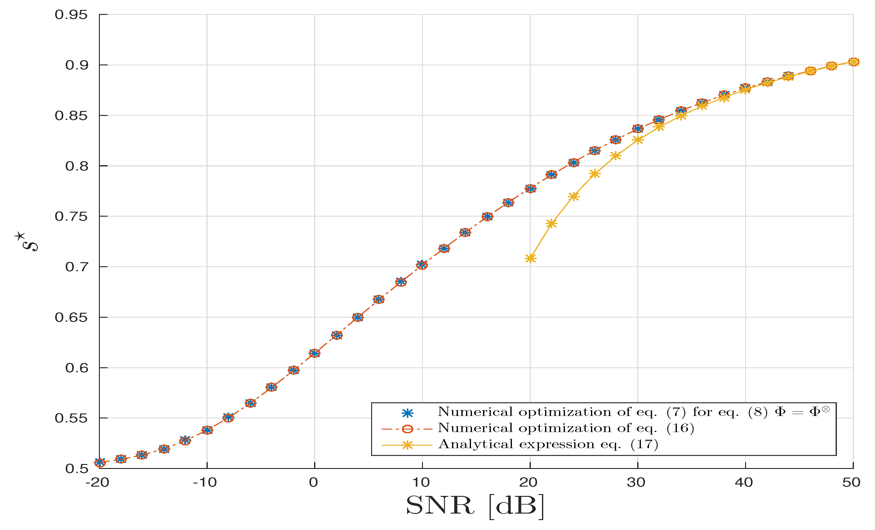
Firstly, for the CPD model, in Figure 4, parameter $s^{\star }$ is drawn with respect to the $\mathrm{SNR}$ in dB. The parameter $s^{\star }$ is obtained thanks to three different methods. The first one is based on the brute force/exhaustive computation of the CUB by minimizing the expression in Equation (8) with $\mathbf{\Phi }={\mathbf{\Phi }}^{\odot }$. This approach has a very high computational cost especially in our asymptotic regime (for a standard computer with Intel Xeon E5-2630 2.3 GHz and 32 GB RAM, it requires 183 h to establish 10,000 simulations). The second approach is based on the numerical optimization of the closed-form expression of $\mu \left(s\right)$ given in Result 4. In this scenario, the drawback in terms of the computational cost is largely mitigated since it consists of a minimization of a univariate regular function. Finally, under the hypothesis that $\mathrm{SNR}$ is large, typically >30 dB, the optimal s-value, $s^{\star }$, is derived by an analytic expression given by Equation (15). We can check that the proposed semi-analytic and analytic expressions are in good agreement with the brute-force method for a lowest computational cost. Moreover, we compute the mean square relative error $\frac{1}{L}{\sum }_{l=1}^L{(\frac{{\widehat{s}}_l^{\star }-s^{\star }}{s^{\star }})}^2$ where L = 10,000 the number of samples for Monte–Carlo process and where ${\widehat{s}}_l^{\star }=arg{min}_{s\in [0,1]}{\mu }_{N,l}\left(s\right)$ and $s^{\star }=arg{min}_{s\in [0,1]}\mu \left(s\right)$. It turns out that the mean square relative errors are in mean of order $-40$ dB. We can conclude that the estimator ${\widehat{s}}^{\star }$ is a consistent estimator of $s^{\star }$.

Figure 4. Canonical Polyadic Decomposition (CPD) scenario: Optimal s-parameter versus Signal to Noise Ratio (SNR) in dB.

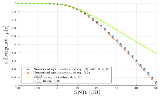
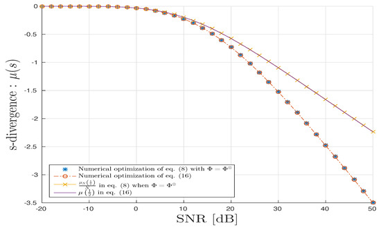
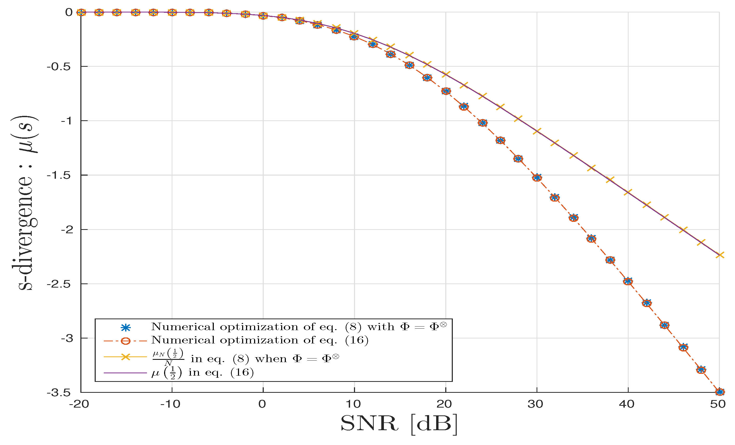
In Figure 5, we draw various s-divergences: $\mu \left(\frac{1}{2}\right),\mu \left(s^{\star }\right),\frac{1}{N}{\mu }_N\left(\frac{1}{2}\right),\frac{1}{N}{\mu }_N\left(\widehat{s}\right)$. We can observe the good agreement with the proposed theoretical results. The s-divergence obtained by fixing $s=\frac{1}{2}$ is accurate only at small $\mathrm{SNR}$ but degrades when $\mathrm{SNR}$ grows large.

Figure 5. CPD scenario: s-divergence vs. $\mathrm{SNR}$ in dB.

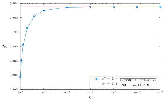
In Figure 6, we fix $\mathrm{SNR}=45$ dB and draw $s^{\star }$ obtained by Equation (14) versus values of $c\in \{{10}^{-6},{10}^{-5},{10}^{-4},{10}^{-3},{10}^{-2},{10}^{-1},0.25,0.5,0.75,0.9,0.99\}$ and the expression obtained by Equation (15). The two curves approach each other as c goes to zero as predicted by our theoretical analysis.

Figure 6. CPD scenario: $s^{\star }$ vs. c , $\mathrm{SNR}=45$ dB.

For the TKD scenario, we follow the same methodology as above for CPD, Figure 7 and Figure 8 all agree with the analysis provided in Section 4.3.

Figure 7. TucKer Decomposition (TKD) scenario: Optimal s-parameter vs. $\mathrm{SNR}$ in dB.

Figure 8. TKD scenario: s-divergence vs. $\mathrm{SNR}$ in dB.

For TKD scenario, the mean square relative error is in mean of order $-40$ dB. So, we check numerically the consistency of the estimator of the optimal s-value.

We can also notice that the convergence of $\frac{{\mu }_N\left(s\right)}{N}$ towards its deterministic equivalent $\mu \left(s\right)$ in the case TKD is faster than in the case CPD, since the dimension of matrix ${\mathbf{\Phi }}^{\otimes }$ is $200,200,200\times 100,120,140$ ($N={200}^3$) which is much larger than the dimension $6000\times 3000$ of ${\mathbf{\Phi }}^{\odot }$ ($N=6000$).

6. Conclusions

In this work, we derived and studied the limit performance in terms of minimal Bayes’ error probability for the binary classification of high-dimensional random tensors using both the tools of Information Geometry (IG) and of Random Matrix Theory (RMT). The main results on Chernoff Bounds and Fisher Information are illustrated by Monte–Carlo simulations that corroborated our theoretical analysis.

For future work, we would like to study the rate of convergence and the fluctuation of the statistics $\frac{{\mu }_N\left(s\right)}{N}$ and $\widehat{s}$.

References

- Besson, O.; Scharf, L.L. CFAR matched direction detector. IEEE Trans. Signal Process. 2006, 54, 2840–2844. [Google Scholar] [CrossRef] [Scilit]
- Bianchi, P.; Debbah, M.; Maida, M.; Najim, J. Performance of Statistical Tests for Source Detection using Random Matrix Theory. IEEE Trans. Inf. Theory 2011, 57, 2400–2419. [Google Scholar] [CrossRef] [Scilit]
- Kay, S.M. Fundamentals of Statistical Signal Processing, Volume II: Detection Theory; PTR Prentice-Hall: Englewood Cliffs, NJ, USA, 1993. [Google Scholar]
- Loubaton, P.; Vallet, P. Almost Sure Localization of the Eigenvalues in a Gaussian Information Plus Noise Model. Application to the Spiked Models. Electron. J. Probab. 2011, 16, 1934–1959. [Google Scholar] [CrossRef] [Scilit]
- Mestre, X. Improved Estimation of Eigenvalues and Eigenvectors of Covariance Matrices Using Their Sample Estimates. IEEE Trans. Inf. Theory 2008, 54, 5113–5129. [Google Scholar] [CrossRef] [Scilit]
- Baik, J.; Silverstein, J. Eigenvalues of large sample covariance matrices of spiked population models. J. Multivar. Anal. 2006, 97, 1382–1408. [Google Scholar] [CrossRef] [Scilit]
- Silverstein, J.W.; Combettes, P.L. Signal detection via spectral theory of large dimensional random matrices. IEEE Trans. Signal Process. 1992, 40, 2100–2105. [Google Scholar] [CrossRef] [Scilit]
- Cheng, Y.; Hua, X.; Wang, H.; Qin, Y.; Li, X. The Geometry of Signal Detection with Applications to Radar Signal Processing. Entropy 2016, 18, 381. [Google Scholar] [CrossRef] [Scilit]
- Ali, S.M.; Silvey, S.D. A General Class of Coefficients of Divergence of One Distribution from Another. J. R. Stat. Soc. Ser. B (Methodol.) 1966, 28, 131–142. [Google Scholar]
- Cover, T.M.; Thomas, J.A. Elements of Information Theory; John Wiley & Sons: Hoboken, NJ, USA, 2012. [Google Scholar]
- Kailath, T. The Divergence and Bhattacharyya Distance Measures in Signal Selection. IEEE Trans. Commun. Technol. 1967, 15, 52–60. [Google Scholar]
- Nielsen, F. Hypothesis Testing, Information Divergence and Computational Geometry; Geometric Science of Information; Springer: Berlin, Germany, 2013; pp. 241–248. [Google Scholar]
- Sinanovic, S.; Johnson, D.H. Toward a theory of information processing. Signal Process. 2007, 87, 1326–1344. [Google Scholar] [CrossRef] [Scilit]
- Chernoff, H. A Measure of Asymptotic Efficiency for Tests of a Hypothesis Based on the sum of Observations. Ann. Math. Stat. 1952, 23, 493–507. [Google Scholar] [CrossRef] [Scilit]
- Nielsen, F. Chernoff information of exponential families. arXiv, 2011; arXiv:1102.2684.
- Chepuri, S.P.; Leus, G. Sparse sensing for distributed Gaussian detection. In Proceedings of the 2015 IEEE International Conference on Acoustics, Speech and Signal Processing (ICASSP), Brisbane, Australia, 19–24 April 2015. [Google Scholar]
- Tang, G.; Nehorai, A. Performance Analysis for Sparse Support Recovery. IEEE Trans. Inf. Theory 2010, 56, 1383–1399. [Google Scholar] [CrossRef] [Scilit]
- Lee, Y.; Sung, Y. Generalized Chernoff Information for Mismatched Bayesian Detection and Its Application to Energy Detection. IEEE Signal Process. Lett. 2012, 19, 753–756. [Google Scholar]
- Grossi, E.; Lops, M. Space-time code design for MIMO detection based on Kullback-Leibler divergence. IEEE Trans. Inf. Theory 2012, 58, 3989–4004. [Google Scholar] [CrossRef] [Scilit]
- Sen, S.; Nehorai, A. Sparsity-Based Multi-Target Tracking Using OFDM Radar. IEEE Trans. Signal Process. 2011, 59, 1902–1906. [Google Scholar] [CrossRef] [Scilit]
- Boyer, R.; Delpha, C. Relative-entropy based beamforming for secret key transmission. In Proceedings of the 2012 IEEE 7th Sensor Array and Multichannel Signal Processing Workshop (SAM), Hoboken, NJ, USA, 17–20 June 2012. [Google Scholar]
- Tran, N.D.; Boyer, R.; Marcos, S.; Larzabal, P. Angular resolution limit for array processing: Estimation and information theory approaches. In Proceedings of the 20th European Signal Processing Conference (EUSIPCO), Bucharest, Romania, 27–31 August 2012. [Google Scholar]
- Katz, G.; Piantanida, P.; Couillet, R.; Debbah, M. Joint estimation and detection against independence. In Proceedings of the Annual Conference on Communication Control and Computing (Allerton), Monticello, IL, USA, 30 September–3 October 2014; pp. 1220–1227. [Google Scholar]
- Nielsen, F. An information-geometric characterization of Chernoff information. IEEE Signal Process. Lett. 2013, 20, 269–272. [Google Scholar] [CrossRef] [Scilit]
- Cichocki, A.; Mandic, D.; De Lathauwer, L.; Zhou, G.; Zhao, Q.; Caiafa, C.; Phan, H.A. Tensor decompositions for signal processing applications: From two-way to multiway component analysis. IEEE Signal Process. Mag. 2015, 32, 145–163. [Google Scholar] [CrossRef] [Scilit]
- Comon, P. Tensors: A brief introduction. IEEE Signal Process. Mag. 2014, 31, 44–53. [Google Scholar] [CrossRef] [Scilit]
- De Lathauwer, L.; Moor, B.D.; Vandewalle, J. A Multilinear Singular Value Decomposition. SIAM J. Matrix Anal. Appl. 2000, 21, 1253–1278. [Google Scholar] [CrossRef] [Scilit]
- Tucker, L.R. Some mathematical notes on three-mode factor analysis. Psychometrika 1966, 31, 279–311. [Google Scholar] [CrossRef] [Scilit] [PubMed]
- Comon, P.; Berge, J.T.; De Lathauwer, L.; Castaing, J. Generic and Typical Ranks of Multi-Way Arrays. Linear Algebra Appl. 2009, 430, 2997–3007. [Google Scholar] [CrossRef] [Scilit]
- De Lathauwer, L. A survey of tensor methods. In Proceedings of the IEEE International Symposium on Circuits and Systems, ISCAS 2009, Taipei, Taiwan, 24–27 May 2009. [Google Scholar]
- Comon, P.; Luciani, X.; De Almeida, A.L.F. Tensor decompositions, alternating least squares and other tales. J. Chemom. 2009, 23, 393–405. [Google Scholar] [CrossRef] [Scilit]
- Goulart, J.H.D.M.; Boizard, M.; Boyer, R.; Favier, G.; Comon, P. Tensor CP Decomposition with Structured Factor Matrices: Algorithms and Performance. IEEE J. Sel. Top. Signal Process. 2016, 10, 757–769. [Google Scholar] [CrossRef] [Scilit]
- Eckart, C.; Young, G. The approximation of one matrix by another of lower rank. Psychometrika 1936, 1, 211–218. [Google Scholar]
- Badeau, R.; Richard, G.; David, B. Fast and stable YAST algorithm for principal and minor subspace tracking. IEEE Trans. Signal Process. 2008, 56, 3437–3446. [Google Scholar] [CrossRef] [Scilit]
- Boyer, R.; Badeau, R. Adaptive multilinear SVD for structured tensors. In Proceedings of the 2006 IEEE International Conference on Acoustics, Speech, and Signal Processing (ICASSP’06), Toulouse, France, 14–19 May 2006. [Google Scholar]
- Boizard, M.; Ginolhac, G.; Pascal, F.; Forster, P. Low-rank filter and detector for multidimensional data based on an alternative unfolding HOSVD: Application to polarimetric STAP. EURASIP J. Adv. Signal Process. 2014, 2014, 119. [Google Scholar] [CrossRef] [Scilit]
- Bouleux, G.; Boyer, R. Sparse-Based Estimation Performance for Partially Known Overcomplete Large-Systems. Signal Process. 2017, 139, 70–74. [Google Scholar] [CrossRef] [Scilit]
- Boyer, R.; Couillet, R.; Fleury, B.-H.; Larzabal, P. Large-System Estimation Performance in Noisy Compressed Sensing with Random Support—A Bayesian Analysis. IEEE Trans. Signal Process. 2016, 64, 5525–5535. [Google Scholar] [CrossRef] [Scilit]
- Ollier, V.; Boyer, R.; El Korso, M.N.; Larzabal, P. Bayesian Lower Bounds for Dense or Sparse (Outlier) Noise in the RMT Framework. In Proceedings of the 2016 IEEE Sensor Array and Multichannel Signal Processing Workshop (SAM 16), Rio de Janerio, Brazil, 10–13 July 2016. [Google Scholar]
- Wishart, J. The generalized product moment distribution in samples. Biometrika 1928, 20A, 32–52. [Google Scholar] [CrossRef] [Scilit]
- Wigner, E.P. On the statistical distribution of the widths and spacings of nuclear resonance levels. Proc. Camb. Philos. Soc. 1951, 47, 790–798. [Google Scholar] [CrossRef] [Scilit]
- Wigner, E.P. Characteristic vectors of bordered matrices with infinite dimensions. Ann. Math. 1955, 62, 548–564. [Google Scholar]
- Bai, Z.D.; Silverstein, J.W. Spectral Analysis of Large Dimensional Random Matrices, 2nd ed.; Springer Series in Statistics; Springer: Berlin, Germany, 2010. [Google Scholar]
- Girko, V.L. Theory of Random Determinants; Kluwer Academic Publishers: Dordrecht, The Netherlands, 1990. [Google Scholar]
- Marchenko, V.A.; Pastur, L.A. Distribution of eigenvalues for some sets of random matrices. Math. Sb. (N.S.) 1967, 72, 507–536. [Google Scholar]
- Voiculescu, D. Limit laws for random matrices and free products. Invent. Math. 1991, 104, 201–220. [Google Scholar] [CrossRef] [Scilit]
- Boyer, R.; Nielsen, F. Information Geometry Metric for Random Signal Detection in Large Random Sensing Systems. In Proceedings of the 2017 IEEE International Conference on Acoustics, Speech, and Signal Processing (ICASSP), New Orleans, LA, USA, 5–9 March 2017. [Google Scholar]
- Boyer, R.; Loubaton, P. Large deviation analysis of the CPD detection problem based on random tensor theory. In Proceedings of the 2017 25th European Association for Signal Processing (EUSIPCO), Kos, Greece, 28 August–2 September 2017. [Google Scholar]
- Lytova, A. Central Limit Theorem for Linear Eigenvalue Statistics for a Tensor Product Version of Sample Covariance Matrices. J. Theor. Prob. 2017, 1–34. [Google Scholar] [CrossRef] [Scilit]
- Tulino, A.M.; Verdu, S. Random Matrix Theory and Wireless Communications; Now Publishers Inc.: Hanover, MA, USA, 2004; Volume 1. [Google Scholar]
- Milne-Thomson, L.M. “Elliptic Integrals” (Chapter 17). In Handbook of Mathematical Functions with Formulas, Graphs, and Mathematical Tables, 9th printing; Abramowitz, M., Stegun, I.A., Eds.; Dover Publications: New York, NY, USA, 1972; pp. 587–607. [Google Scholar]
- Behrens, R.T.; Scharf, L.L. Signal processing applications of oblique projection operators. IEEE Trans. Signal Process. 1994, 42, 1413–1424. [Google Scholar] [CrossRef] [Scilit]
- Pajor, A.; Pastur, L.A. On the Limiting Empirical Measure of the sum of rank one matrices with log-concave distribution. Stud. Math. 2009, 195, 11–29. [Google Scholar] [CrossRef] [Scilit]
- Ambainis, A.; Harrow, A.W.; Hastings, M.B. Random matrix theory: Extending random matrix theory to mixtures of random product states. Commun. Math. Phys. 2012, 310, 25–74. [Google Scholar] [CrossRef] [Scilit]
© 2018 by the authors. Licensee MDPI, Basel, Switzerland. This article is an open access article distributed under the terms and conditions of the Creative Commons Attribution (CC BY) license (http://creativecommons.org/licenses/by/4.0/).